The document is a student's homework solution for obtaining a fourth-order Butterworth bandstop filter function and realization. It first derives the transfer function using tables to get maximally flat characteristics at 0 and infinity frequency. It then obtains a passive LC network realization by transforming the lowpass function impedance. Finally, it designs a circuit with components scaled to a 50 ohm load and 1 kHz rejection frequency, and plots the magnitude response.
![Collins, Steven ID#3678
EE175 Web Project
Spring 2009
Professor Strasilla
Problem: Obtain the four-pole BS function that has maximally flat characteristics at ω = 0 and
ω = ∞. The bandwidth taken between the 1-dB down frequencies is to be 0.1ωm. Obtain a passive
realization for the fourth-order BS function, with a 50Ω load resistor.
Plan: The plan for this problem is to first obtain the transfer function and then the realization. To
solve for the transfer function, first solve for the normalized LP function. Next, de-normalize the
function for the pass-band ripple, rejection frequency and then finally transform the function into
the BS function. To obtain the realization, we will use the impedance of the LP function and
transform it into the BS impedance. From there we will construct the circuit.
Solution: Using Table 17.1 in Budak (p. 511, Budak), construct the 3-dB ripple, low-pass
Buttersworth transfer function:
1
3 () =
2 + 2 + 1
To convert the pass-band ripple from 3 dB to 1dB, replace s with s = . 5089 = 0.7133.
1
1 () =
(0.7133)2 + 2(0.7133) + 1
0.1
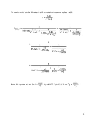
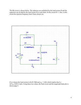
To obtain the frequency-normalized (with respect to ωm) BS function, replace s with s = ( 2 +1):
( 2 + 1)2
=
0.1 2 0.1
(0.7133 ) + 2 0.7133 2 +1
2 + 1 + 1
( 2 + 1)2
=
4 + 0.1009 3 + 2.0021 2 + 0.1009 + 1
( 2 + 1)2
=
+ 0.246 2 + 0.97482 [ + 0.0259 2 + 1.02522 ]
The resulting equation has the desired BS characteristics at ωm = 1. To move the rejection to
ω = ωm, replace s by s/ωm:
1](https://image.slidesharecdn.com/ee175webprojectoriginal-091031210707-phpapp01/85/Ee175webproject-Original-1-320.jpg)
![Collins, Steven ID#3678
EE175 Web Project
Spring 2009
Professor Strasilla
Problem: Obtain the four-pole BS function that has maximally flat characteristics at ω = 0 and
ω = ∞. The bandwidth taken between the 1-dB down frequencies is to be 0.1ωm. Obtain a passive
realization for the fourth-order BS function, with a 50Ω load resistor.
Plan: The plan for this problem is to first obtain the transfer function and then the realization. To
solve for the transfer function, first solve for the normalized LP function. Next, de-normalize the
function for the pass-band ripple, rejection frequency and then finally transform the function into
the BS function. To obtain the realization, we will use the impedance of the LP function and
transform it into the BS impedance. From there we will construct the circuit.
Solution: Using Table 17.1 in Budak (p. 511, Budak), construct the 3-dB ripple, low-pass
Buttersworth transfer function:
1
3 () =
2 + 2 + 1
To convert the pass-band ripple from 3 dB to 1dB, replace s with s = . 5089 = 0.7133.
1
1 () =
(0.7133)2 + 2(0.7133) + 1
0.1
To obtain the frequency-normalized (with respect to ωm) BS function, replace s with s = ( 2 +1):
( 2 + 1)2
=
0.1 2 0.1
(0.7133 ) + 2 0.7133 2 +1
2 + 1 + 1
( 2 + 1)2
=
4 + 0.1009 3 + 2.0021 2 + 0.1009 + 1
( 2 + 1)2
=
+ 0.246 2 + 0.97482 [ + 0.0259 2 + 1.02522 ]
The resulting equation has the desired BS characteristics at ωm = 1. To move the rejection to
ω = ωm, replace s by s/ωm:
1](https://image.slidesharecdn.com/ee175webprojectoriginal-091031210707-phpapp01/75/Ee175webproject-Original-1-2048.jpg)
![[(ω )2 + 1]2
m
= 2
+. 097482 [( + 0.0259)2 + 0.102522 ]
+ 0.0246
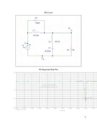
This is the first part of the problem. The next part is to obtain a passive realization. The poles of
this function are complex, and therefore the system is an LC network.
From the low-pass 1 dB equation:
1 1 1 1
1 = 2 + 1.9652) + 1.9824
=
0.5089 ( 0.5089 +
To construct the LP network with resistive load termination, divide the odd part of the
denominator by the even part, since n is even. This will give Z LP2LC.
1.9824 1
2 = =
2+ 1.9652 0.5044 + 1
1.008
With this impedance equation, it is obvious that L=0.5044 and C=1.008. The LP network is
shown below:
2](https://image.slidesharecdn.com/ee175webprojectoriginal-091031210707-phpapp01/85/Ee175webproject-Original-2-320.jpg)