Modu

1. September 2, 2009 ECE 366, Fall 2009
Introduction to ECE 366
Selin Aviyente
Associate Professor

2. September 2, 2009 ECE 366, Fall 2009
Overview
• Lectures: M,W,F 8:00-8:50 a.m.,
1257 Anthony Hall
• Web Page:
http://www.egr.msu.edu/~aviyente/ece366_09
• Textbook: Linear Systems and Signals, Lathi ,
2nd Edition, Oxford Press.
• Office Hours: M,W 3:00-4:30 p.m., 2210
Engineering Building
• Pre-requisites: ECE 202, 280

3. September 2, 2009 ECE 366, Fall 2009
Course Requirements
• 2 Midterm Exams-40%
– October 16th
– November 20th
• Weekly HW Assignments-10%
– Assigned Friday due next Friday (except during exam
weeks)
– Will include MATLAB assignments.
– Should be your own work.
– No late HWs will be accepted.
– Lowest HW grade is dropped.
• Final Project-15% (MATLAB based project)
• Final Exam-35%, December 15th

4. September 2, 2009 ECE 366, Fall 2009
Policies
• Cheating in any form will not be tolerated.
This includes copying HWs, cheating on
exams.
• You are allowed to discuss the HW
questions with your friends, and me.
• However, you have to write up the
homework solutions on your own.
• Lowest HW grade will be dropped.

5. September 2, 2009 ECE 366, Fall 2009
Course Outline
• Part 1- Continuous Time Signals and
Systems
– Basic Signals and Systems Concepts
– Time Domain Analysis of Linear Time
Invariant (LTI) Systems
– Frequency Domain Analysis of Signals and
Systems
• Fourier Series
• Fourier Transform
• Applications

6. September 2, 2009 ECE 366, Fall 2009
Course Outline
• Part 2- Discrete Time Signals and
Systems
– Basic DT Signals and Systems Concepts
– Time Domain Analysis of DT Systems
– Frequency Domain Analysis of DT Signals
and Systems
• Z-transforms
• DTFT

7. September 2, 2009 ECE 366, Fall 2009
Signals
• A signal is a function of one or more variables that
conveys information about a physical phenomenon.
• Signals are functions of independent variables; time (t)
or space (x,y)
• A physical signal is modeled using mathematical
functions.
• Examples:
– Electrical signals: Voltages/currents in a circuit v(t),i(t)
– Temperature (may vary with time/space)
– Acoustic signals: audio/speech signals (varies with time)
– Video (varies with time and space)
– Biological signals: Heartbeat, EEG

8. September 2, 2009 ECE 366, Fall 2009
Systems
• A system is an entity that manipulates one or more
signals that accomplish a function, thereby yielding new
signals.
• The input/output relationship of a system is modeled
using mathematical equations.
• We want to study the response of systems to signals.
• A system may be made up of physical components
(electrical, mechanical, hydraulic) or may be an
algorithm that computes an output from an input signal.
• Examples:
– Circuits (Input: Voltage, Output: Current)
• Simple resistor circuit:
– Mass Spring System (Input: Force, Output: displacement)
– Automatic Speaker Recognition (Input: Speech, Output: Identity)
)
(
)
( t
Ri
t
v 

9. September 2, 2009 ECE 366, Fall 2009
Applications of Signals and
Systems
• Acoustics: Restore speech in a noisy environment such
as cockpit
• Communications: Transmission in mobile phones, GPS,
radar and sonar
• Multimedia: Compress signals to store data such as
CDs, DVDs
• Biomedical: Extract information from biological signals:
– Electrocardiogram (ECG) electrical signals generated by the
heart
– Electroencephalogram (EEG) electrical signals generated by the
brain
– Medical Imaging
• Biometrics: Fingerprint identification, speaker
recognition, iris recognition

10. September 2, 2009 ECE 366, Fall 2009
Classification of Signals
• One-dimensional vs. Multi-dimensional:
The signal can be a function of a single
variable or multiple variables.
– Examples:
• Speech varies as a function of timeone-
dimensional
• Image intensity varies as a function of (x,y)
coordinatesmulti-dimensional
– In this course, we focus on one-dimensional
signals.

11. September 2, 2009 ECE 366, Fall 2009
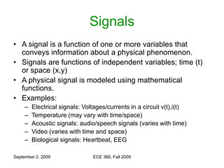
• Continuous-time vs. discrete-time:
– A signal is continuous time if it is defined for
all time, x(t).
– A signal is discrete time if it is defined only at
discrete instants of time, x[n].
– A discrete time signal is derived from a
continuous time signal through sampling, i.e.:
period
sampling
is
T
nT
x
n
x s
s ),
(
]
[ 

12. September 2, 2009 ECE 366, Fall 2009
• Analog vs. Digital:
– A signal whose amplitude can take on any
value in a continuous range is an analog
signal.
– A digital signal is one whose amplitude can
take on only a finite number of values.
– Example: Binary signals are digital signals.
– An analog signal can be converted into a
digital signal through quantization.

13. September 2, 2009 ECE 366, Fall 2009
• Deterministic vs. Random:
– A signal is deterministic if we can define its
value at each time point as a mathematical
function
– A signal is random if it cannot be described by
a mathematical function (can only define
statistics)
– Example:
• Electrical noise generated in an amplifier of a
radio/TV receiver.

14. September 2, 2009 ECE 366, Fall 2009
• Periodic vs. Aperiodic Signals:
– A periodic signal x(t) is a function of time that satisfies
– The smallest T, that satisfies this relationship is called
the fundamental period.
– is called the frequency of the signal (Hz).
– Angular frequency, (radians/sec).
– A signal is either periodic or aperiodic.
– A periodic signal must continue forever.
– Example: The voltage at an AC power source is
periodic.
)
(
)
( T
t
x
t
x 

T
f
1

  
 


0 0
0
)
(
)
(
)
(
T
a
a
T
b
b T
dt
t
x
dt
t
x
dt
t
x
T
f



2
2 


15. September 2, 2009 ECE 366, Fall 2009
• Causal, Anticausal vs. Noncausal Signals:
– A signal that does not start before t=0 is a
causal signal. x(t)=0, t<0
– A signal that starts before t=0 is a noncausal
signal.
– A signal that is zero for t>0 is called an
anticausal signal.

16. September 2, 2009 ECE 366, Fall 2009
• Even vs. Odd:
– A signal is even if x(t)=x(-t).
– A signal is odd if x(t)=-x(-t)
– Examples:
• Sin(t) is an odd signal.
• Cos(t) is an even signal.
– A signal can be even, odd or neither.
– Any signal can be written as a combination of
an even and odd signal.
2
)
(
)
(
)
(
2
)
(
)
(
)
(
t
x
t
x
t
x
t
x
t
x
t
x
o
e







17. September 2, 2009 ECE 366, Fall 2009
Properties of Even and Odd
Functions
• Even x Odd = Odd
• Odd x Odd = Even
• Even x Even = Even
• Even + Even = Even
• Even + Odd = Neither
• Odd + Odd = Odd
0
)
(
)
(
2
)
(
0







dt
t
x
dt
t
x
dt
t
x
a
a
o
a
e
a
a
e

18. September 2, 2009 ECE 366, Fall 2009
• Finite vs. Infinite Length:
– X(t) is a finite length signal if it is nonzero over
a finite interval a<t<b
– X(t) is infinite length signal if it is nonzero over
all real numbers.
– Periodic signals are infinite length.

19. September 2, 2009 ECE 366, Fall 2009
• Energy signals vs. power signals:
– Consider a voltage v(t) developed across a
resistor R, producing a current i(t).
– The instantaneous power: p(t)=v2(t)/R=Ri2(t)
– In signal analysis, the instantaneous power of
a signal x(t) is equivalent to the instantaneous
power over 1 resistor and is defined as x2(t).
– Total Energy:
– Average Power: 



2
/
2
/
2
)
(
1
lim
T
T
T dt
t
x
T




2
/
2
/
2
)
(
lim
T
T
T dt
t
x

20. September 2, 2009 ECE 366, Fall 2009
• Energy vs. Power Signals:
– A signal is an energy signal if its energy is finite,
0<E<∞.
– A signal is a power signal if its power is finite, 0<P<∞.
– An energy signal has zero power, and a power signal
has infinite energy.
– Periodic signals and random signals are usually
power signals.
– Signals that are both deterministic and aperiodic are
usually energy signals.
– Finite length and finite amplitude signals are energy
signals.