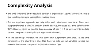
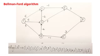
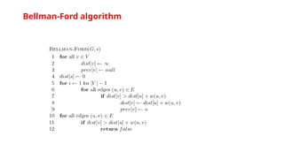
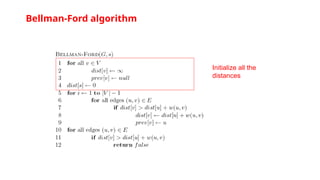
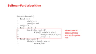
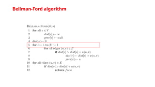
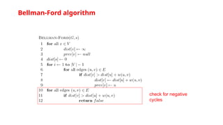
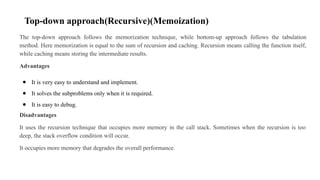
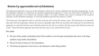
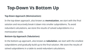
Dynamic programming in Design Analysis and Algorithms

Dynamic programming
Dr. G.L. Saini

Dynamic Programming
Dynamic programming approach is similar to divide and conquer in breaking down the problem into
smaller and yet smaller possible sub-problems. But unlike, divide and conquer, these sub-problems are
not solved independently. Rather, results of these smaller sub-problems are remembered and used for
similar or overlapping sub-problems.
Dynamic programming is used where we have problems, which can be divided into similar sub-
problems, so that their results can be re-used. Mostly, these algorithms are used for optimization.
Before solving the in-hand sub-problem, dynamic algorithm will try to examine the results of the
previously solved sub-problems. The solutions of sub-problems are combined in order to achieve the
best solution.
So we can say that −
● The problem should be able to be divided into smaller overlapping sub-problem.
● An optimum solution can be achieved by using an optimum solution of smaller sub-problems.
● Dynamic algorithms use Memoization.

Comparison
In contrast to greedy algorithms, where local optimization is addressed, dynamic
algorithms are motivated for an overall optimization of the problem.
In contrast to divide and conquer algorithms, where solutions are combined to achieve an
overall solution, dynamic algorithms use the output of a smaller sub-problem and then try
to optimize a bigger sub-problem. Dynamic algorithms use Memoization to remember the
output of already solved sub-problems.
Example
The following computer problems can be solved using dynamic programming approach −
● Shortest path by Bellman ford
● Knapsack problem
● All pair shortest path by Floyd-Warshall
● Matrix chain multiplication
● Fibonacci number series etc.

How does the dynamic programming approach work?
The following are the steps that the dynamic programming follows:
● It breaks down the complex problem into simpler subproblems.
● It finds the optimal solution to these sub-problems.
● It stores the results of subproblems (memoization). The process of storing the results of subproblems is known as memorization.
● It reuses them so that same sub-problem is calculated more than once.
● Finally, calculate the result of the complex problem.
The above five steps are the basic steps for dynamic programming. The dynamic programming is applicable that are having properties
such as:
Those problems that are having overlapping subproblems and optimal substructures. Here, optimal substructure means that the solution of
optimization problems can be obtained by simply combining the optimal solution of all the subproblems.
In the case of dynamic programming, the space complexity would be increased as we are storing the intermediate results, but the time
complexity would be decreased.
There are two approaches to dynamic programming:
● Top-down approach
● Bottom-up approach

Top-down approach(Recursive)(Memoization)
The top-down approach follows the memorization technique, while bottom-up approach follows the tabulation
method. Here memorization is equal to the sum of recursion and caching. Recursion means calling the function itself,
while caching means storing the intermediate results.
Advantages
● It is very easy to understand and implement.
● It solves the subproblems only when it is required.
● It is easy to debug.
Disadvantages
It uses the recursion technique that occupies more memory in the call stack. Sometimes when the recursion is too
deep, the stack overflow condition will occur.
It occupies more memory that degrades the overall performance.

Bottom-Up approach(Iterative)(Tabulation)
The bottom-up approach is also one of the techniques which can be used to implement the dynamic programming. It uses
the tabulation technique to implement the dynamic programming approach. It solves the same kind of problems but it
removes the recursion. If we remove the recursion, there is no stack overflow issue and no overhead of the recursive
functions. In this tabulation technique, we solve the problems and store the results in a matrix.
The bottom-up is the approach used to avoid the recursion, thus saving the memory space. The bottom-up is an algorithm
that starts from the beginning, whereas the recursive algorithm starts from the end and works backward. In the bottom-up
approach, we start from the base case to find the answer for the end. As we know, the base cases in the Fibonacci series are
0 and 1. Since the bottom approach starts from the base cases, so we will start from 0 and 1.
Key points
● We solve all the smaller sub-problems that will be needed to solve the larger sub-problems then move to the larger
problems using smaller sub-problems.
● We use for loop to iterate over the sub-problems.
● The bottom-up approach is also known as the tabulation or table filling method.

Top-Down Vs Bottom Up
Top-Down Approach (Memoization):
In the top-down approach, also known as memoization, we start with the final
solution and recursively break it down into smaller subproblems. To avoid
redundant calculations, we store the results of solved subproblems in a
memoization table.
Bottom-Up Approach (Tabulation):
In the bottom-up approach, also known as tabulation, we start with the smallest
subproblems and gradually build up to the final solution. We store the results of
solved subproblems in a table to avoid redundant calculations.

Fibonacci Numbers using Dynamic Programming
The recursive solution is more elegant:
function fib(n){
if (n < 0) return undefined;
if (n < 2) return n;
return fib(n-1) + fib(n-2)
}
but its time complexity is exponential, or O(2^n), which is not
ideal at all.

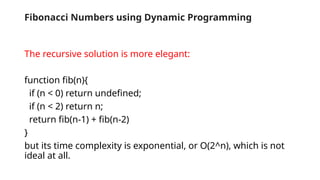
This is a bottom-up approach. We start from the bottom, finding fib(0) and fib(1), add them together to
get fib(2) and so on until we reach fib(5).
function tabulatedFib(n)
{
if (n === 1 || n === 2){
return 1;
}
const fibNums = [0, 1, 1];
for (let i = 3; i <= n; i++){
fibNums[i] = fibNums[i-1] + fibNums[i-2];
}
return fibNums[n];
}
The time complexity of both the memoization and tabulation solutions are O(n) — time grows linearly
with the size of n, because we are calculating fib(4), fib(3), etc each one time.
Fibonacci Numbers using Dynamic Programming (Bottom Up)

Complexity Analysis
• The time complexity of the recursive solution is exponential – O(2^N) to be exact. This is
due to solving the same subproblems multiple times.
• For the top-down approach, we only solve each subproblem one time. Since each
subproblem takes a constant amount of time to solve, this gives us a time complexity of
O(N). However, since we need to keep an array of size N + 1 to save our intermediate
results, the space complexity for this algorithm is also O(N).
• In the bottom-up approach, we also solve each subproblem only once. So the time
complexity of the algorithm is also O(N). Since we only use two variables to track our
intermediate results, our space complexity is constant, O(1).

Initialize all the
distances
Bellman-Ford algorithm

iterate over all
edges/vertices
and apply update
rule

check for negative
cycles

Negative cycles
A
B
C E
D
1
1
-10
5
10
3
What is the shortest path
from a to e?

Dynamic programming in Design Analysis and Algorithms

More Related Content

Similar to Dynamic programming in Design Analysis and Algorithms

Recently uploaded

Dynamic programming in Design Analysis and Algorithms