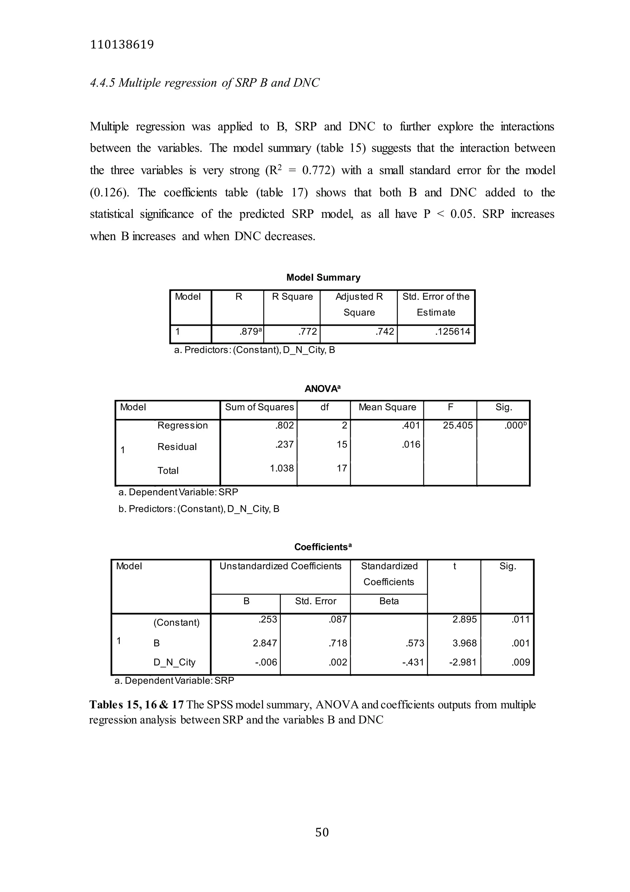
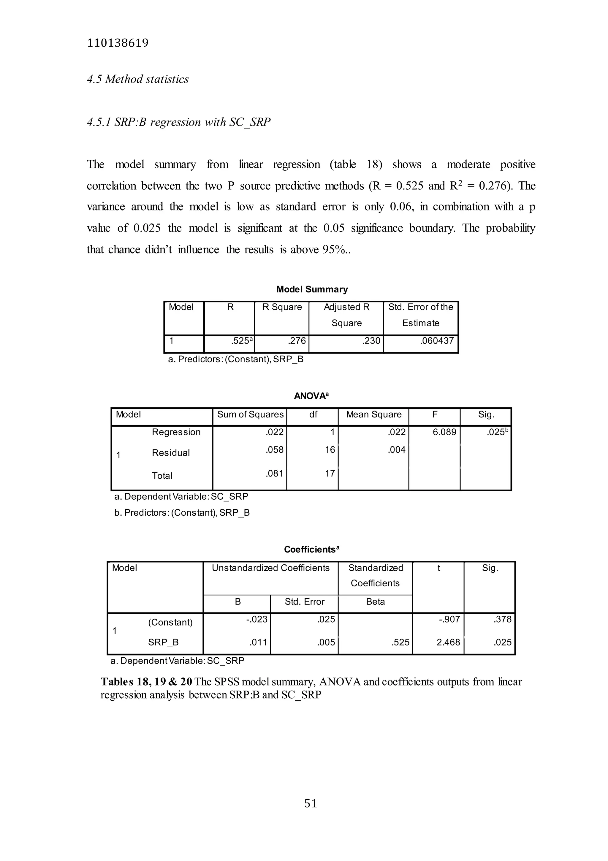
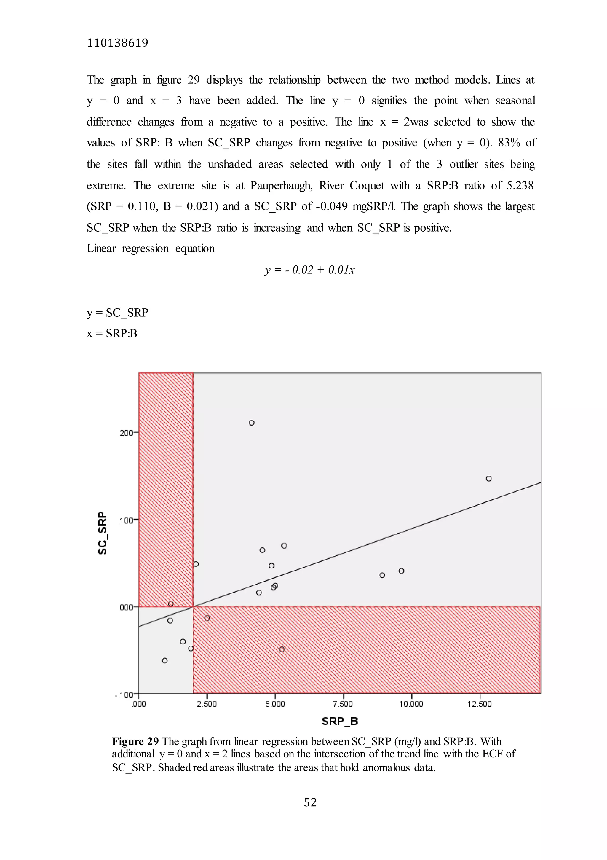
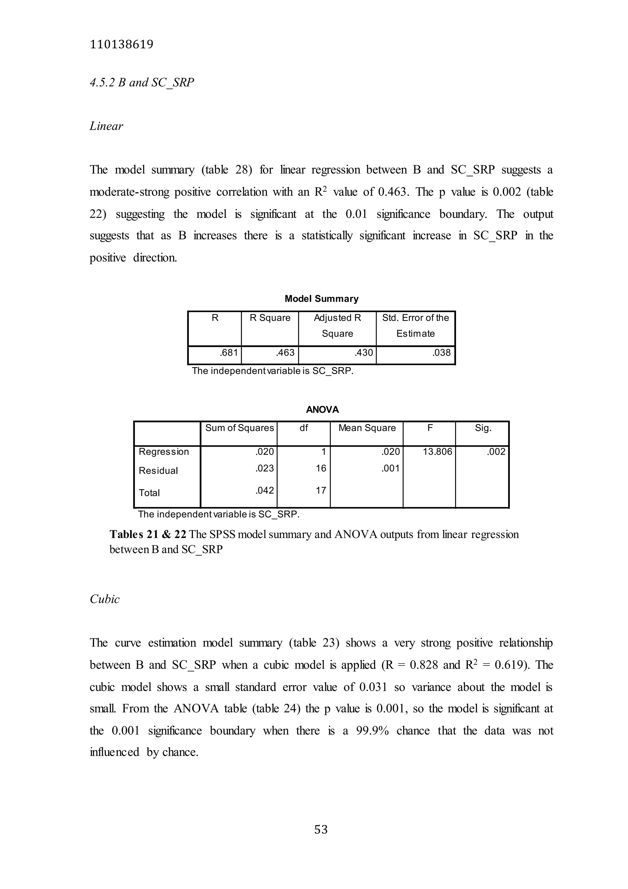
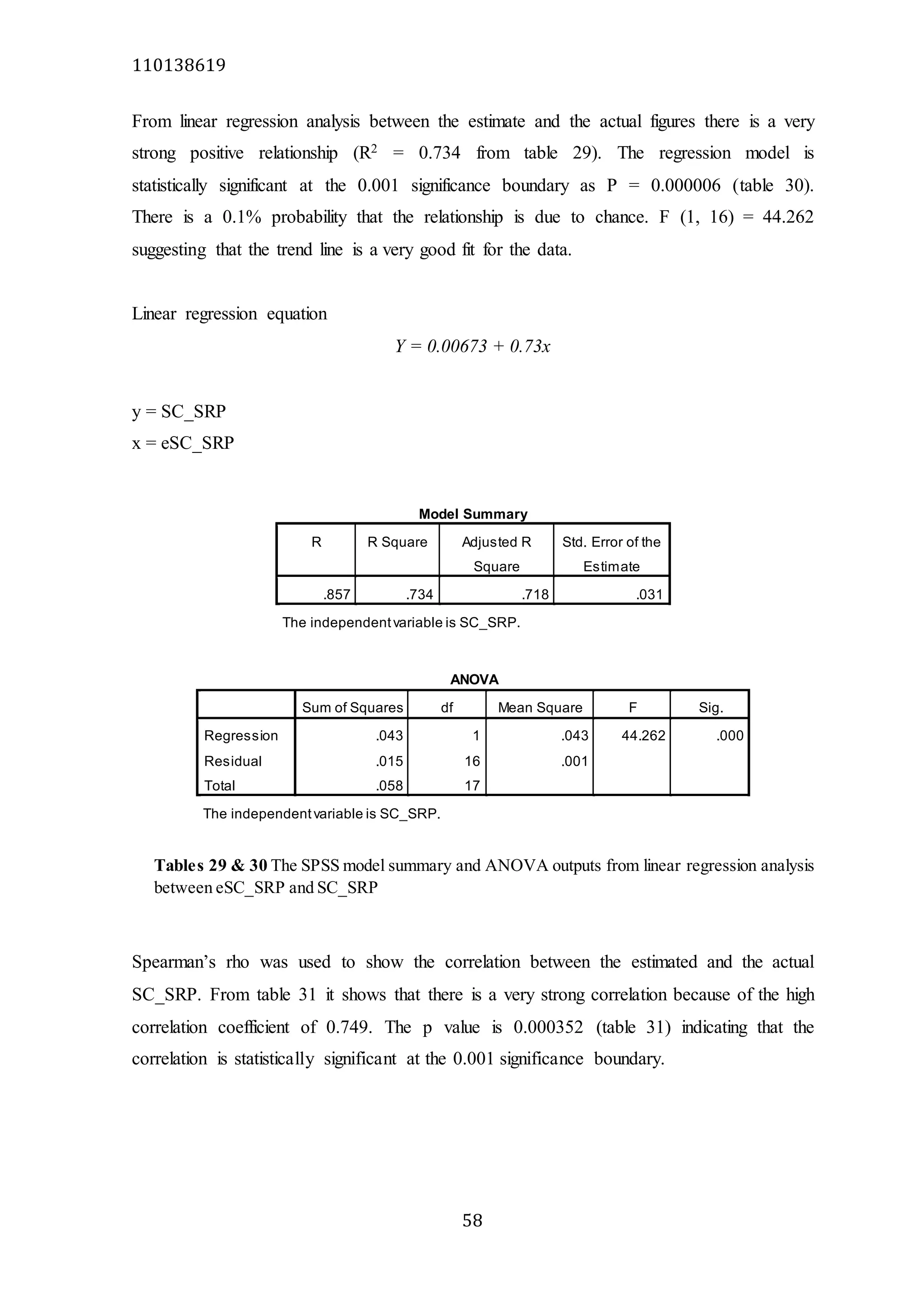
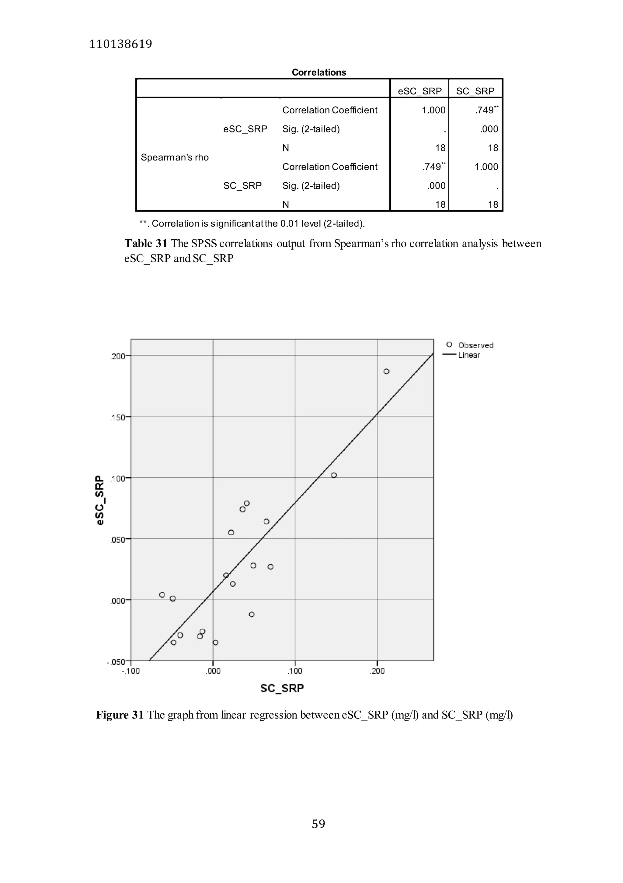
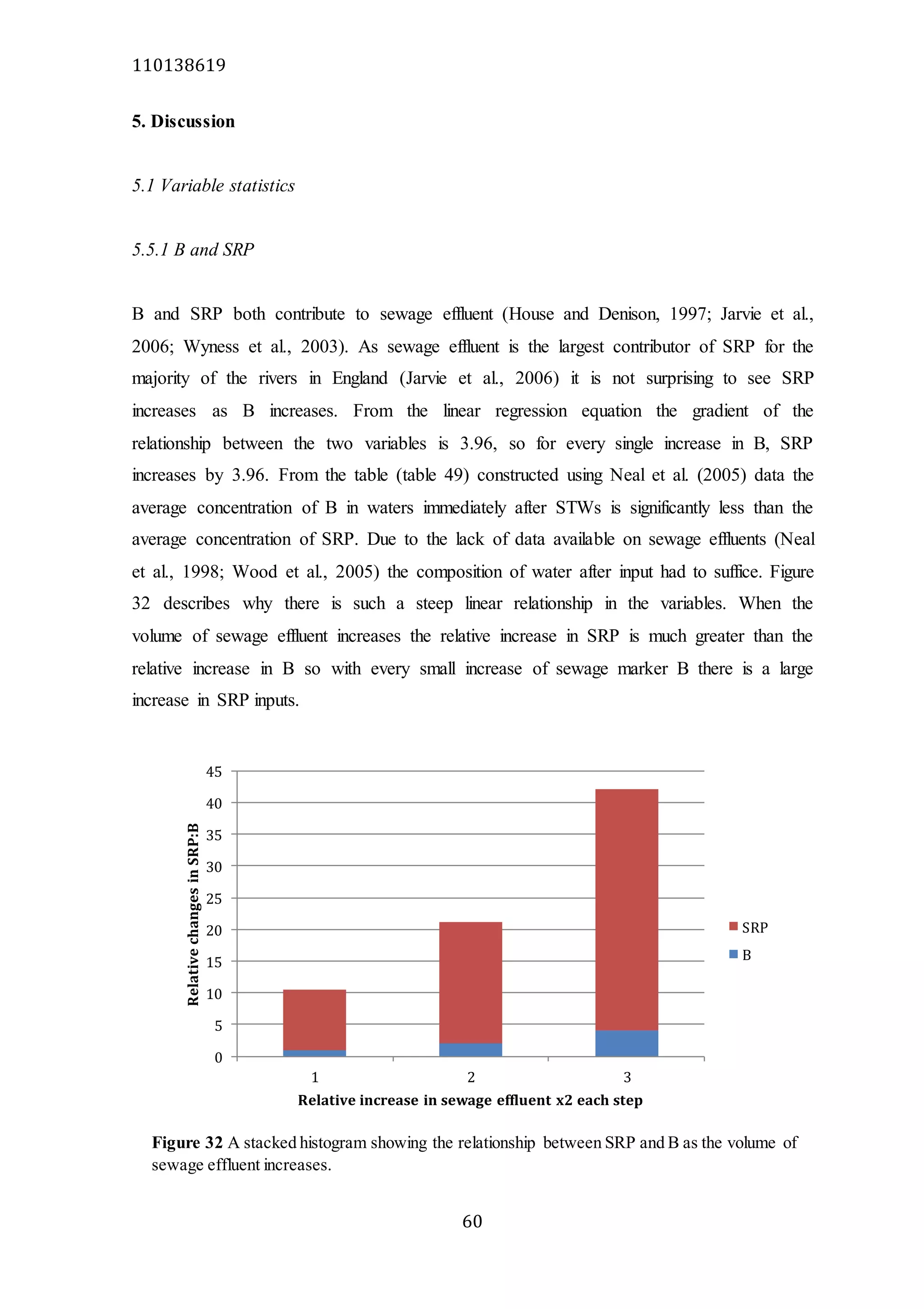
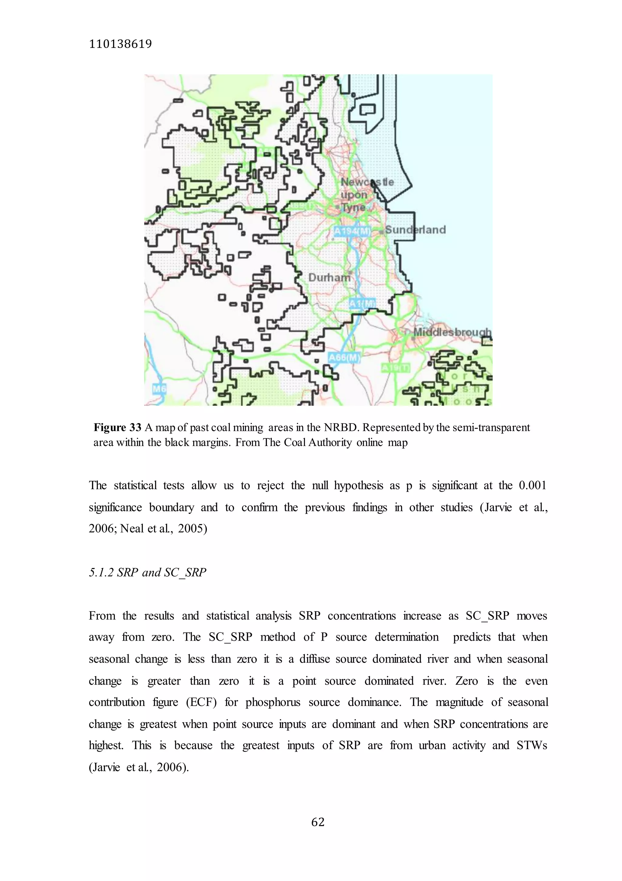
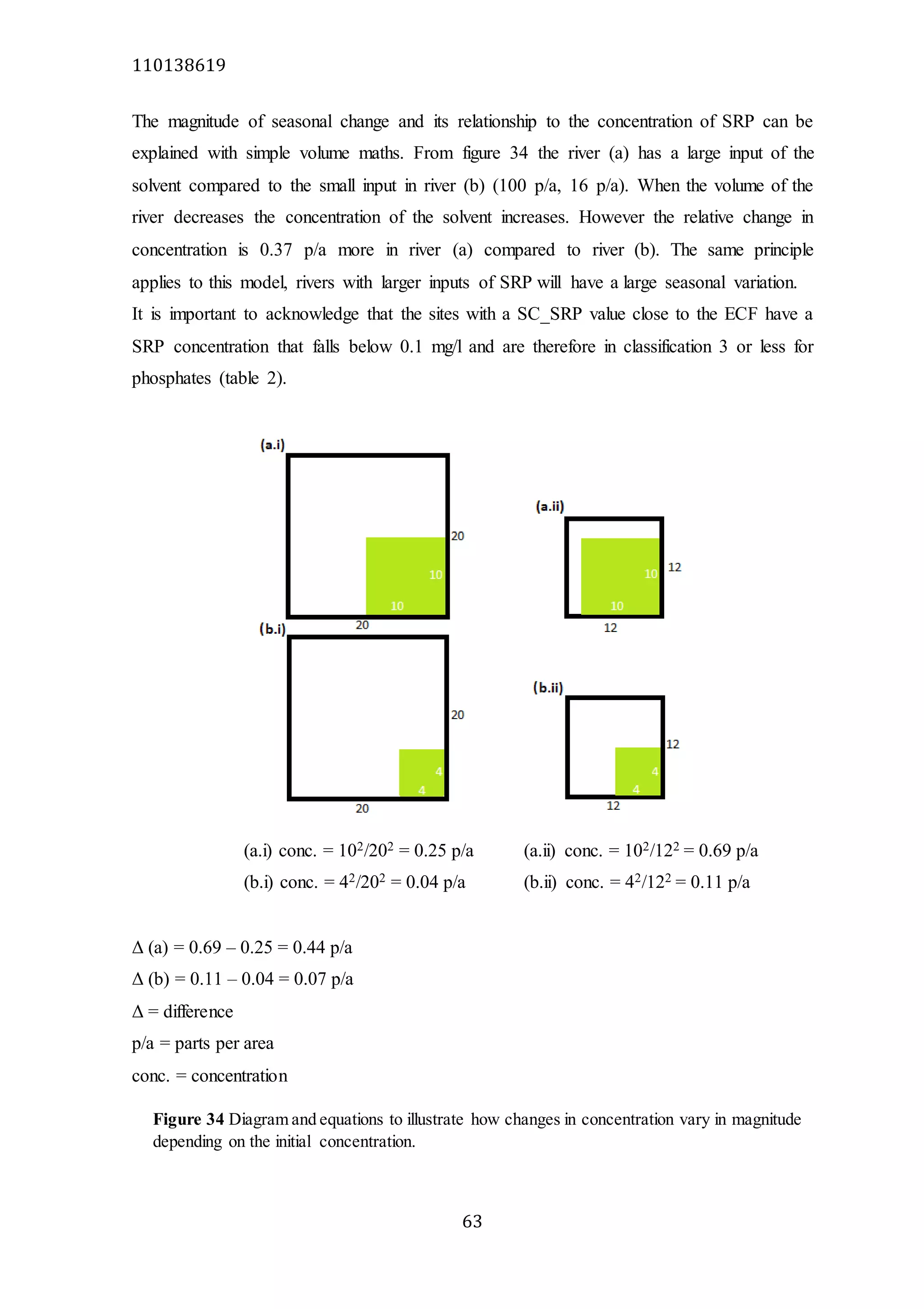
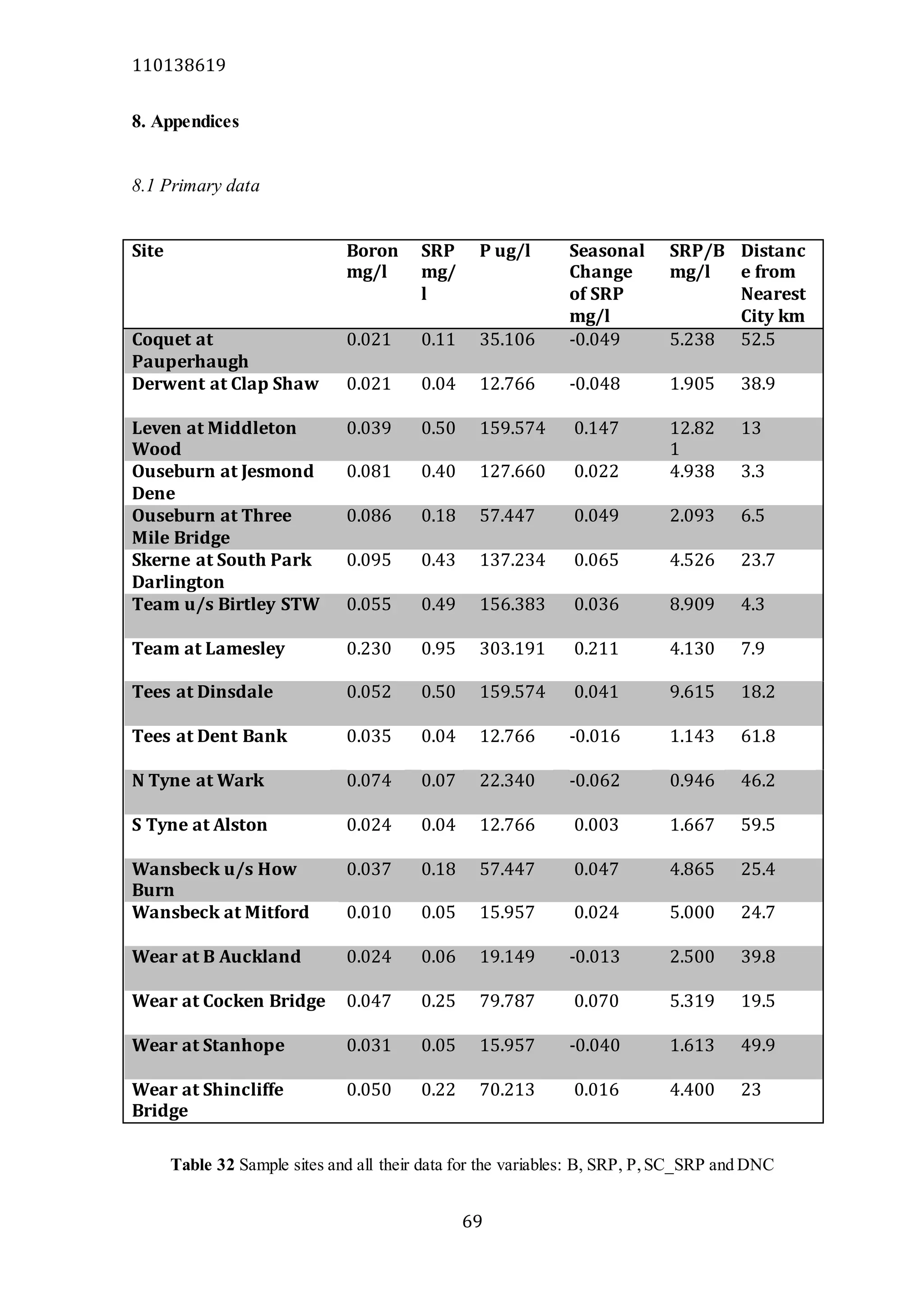
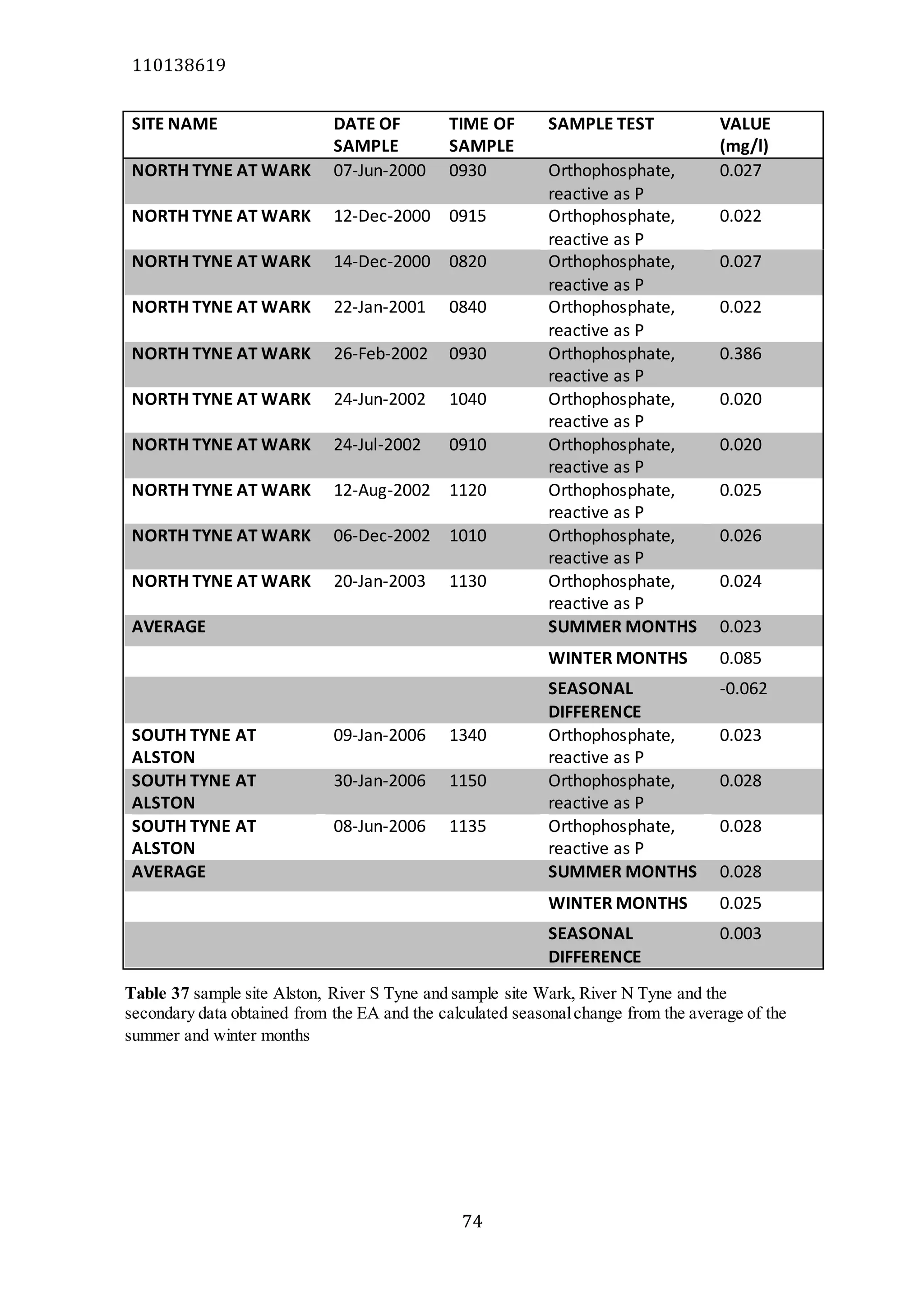
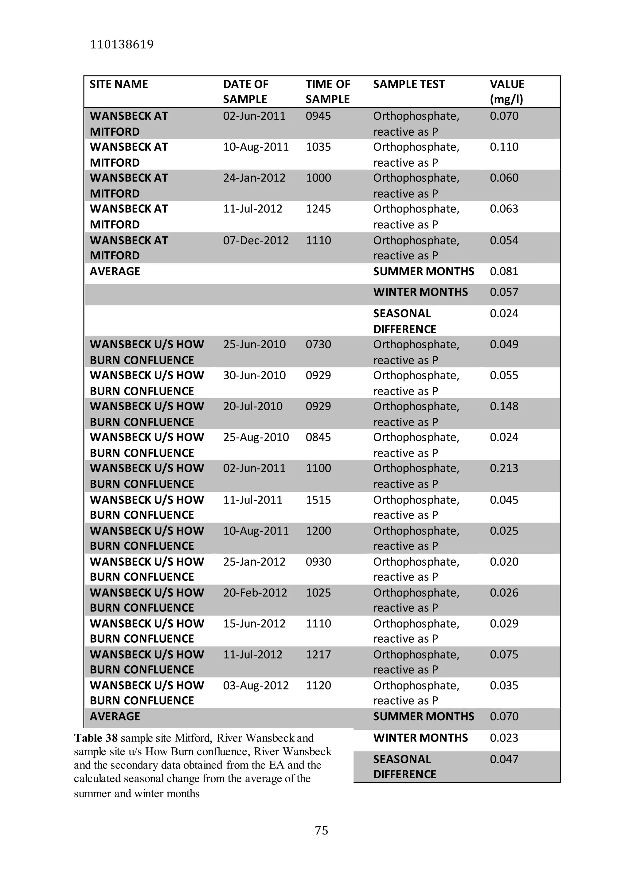
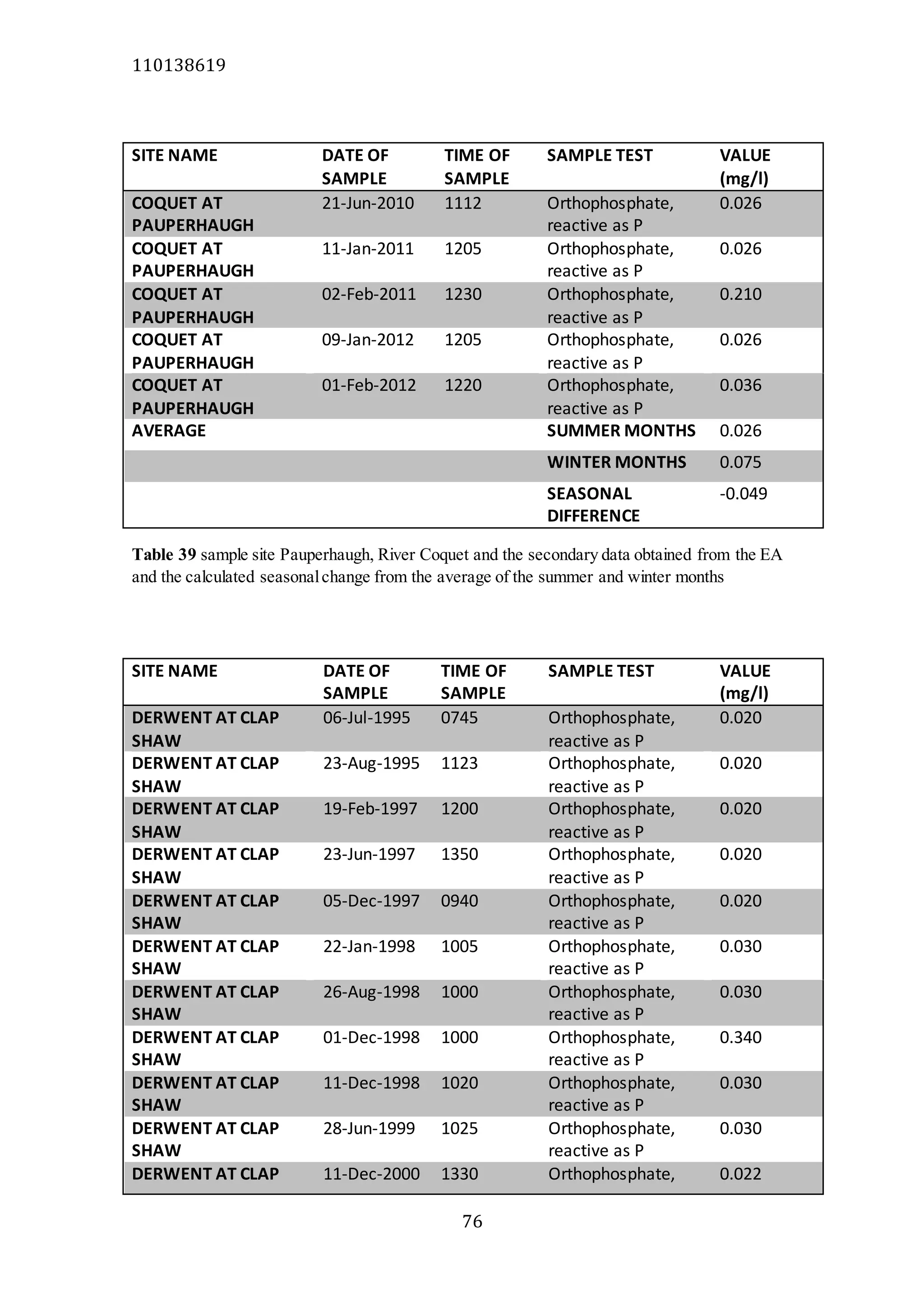
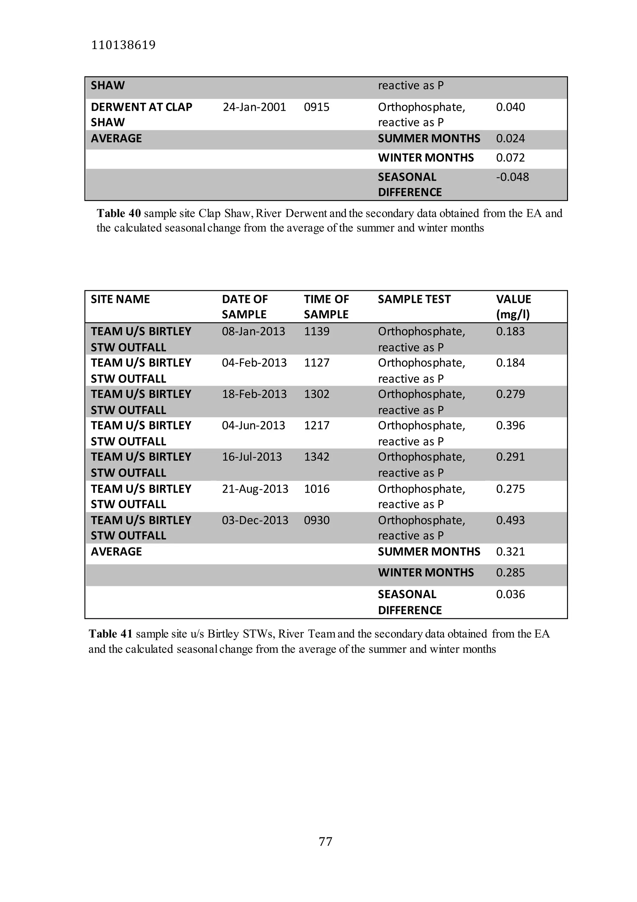
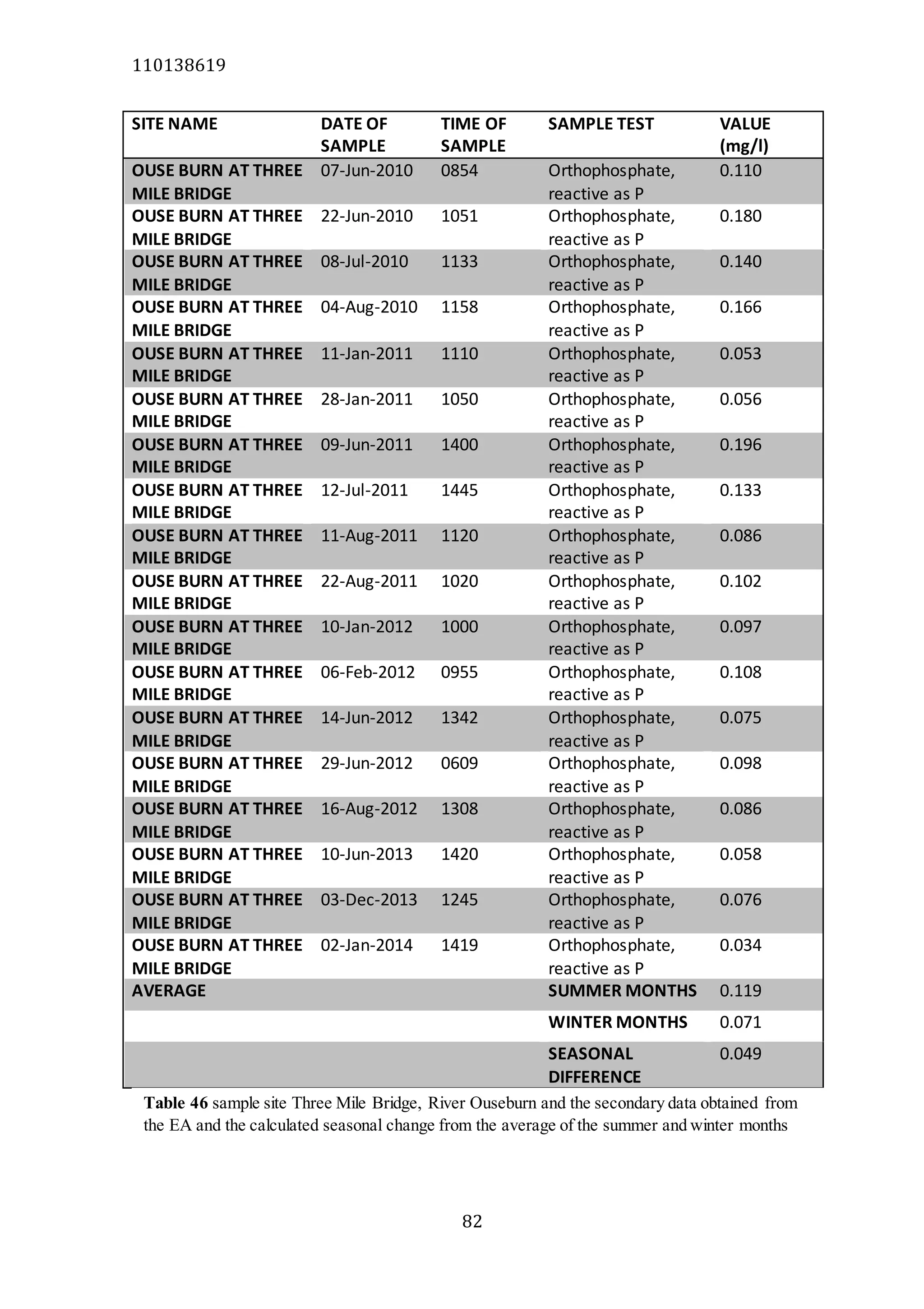
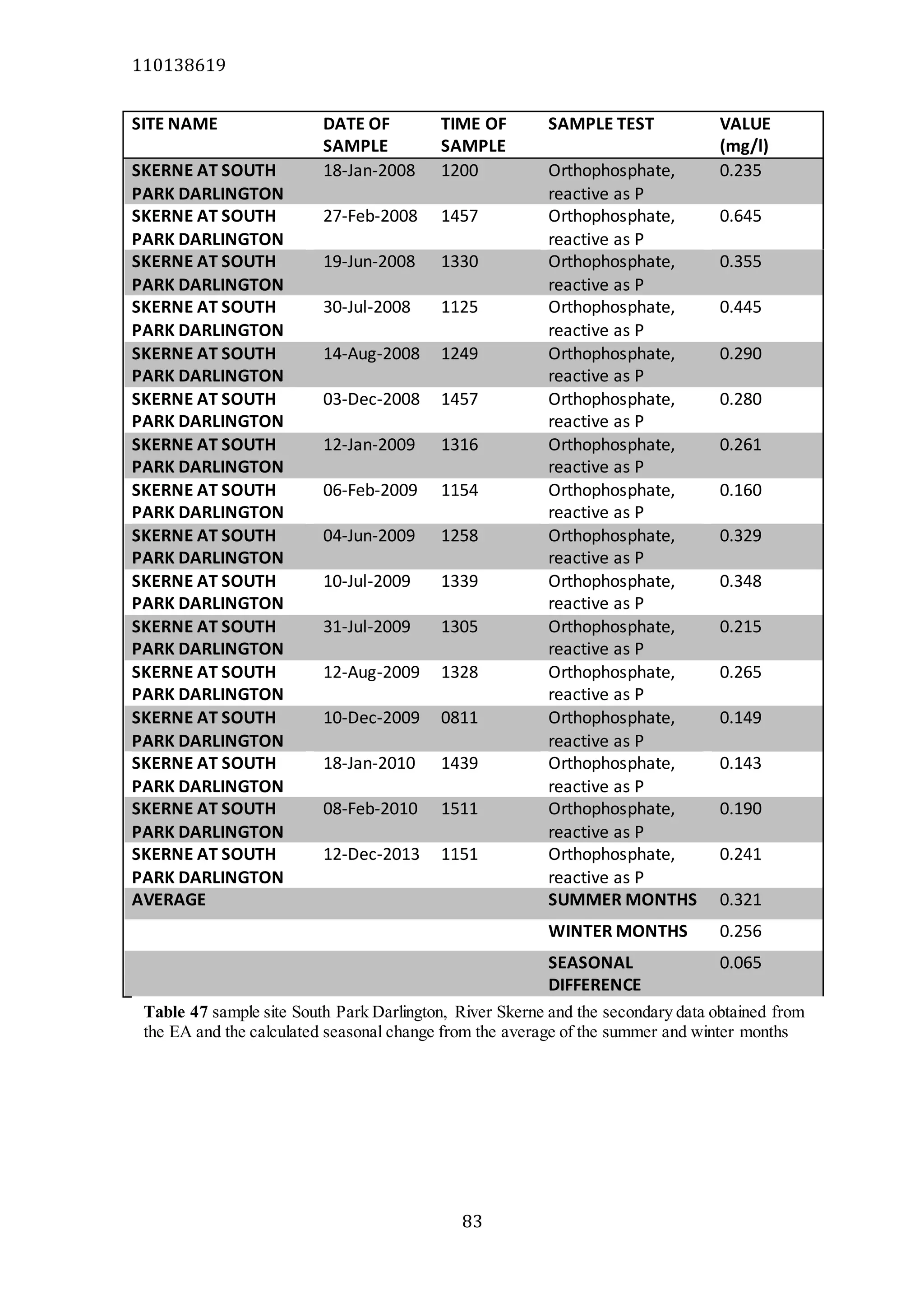
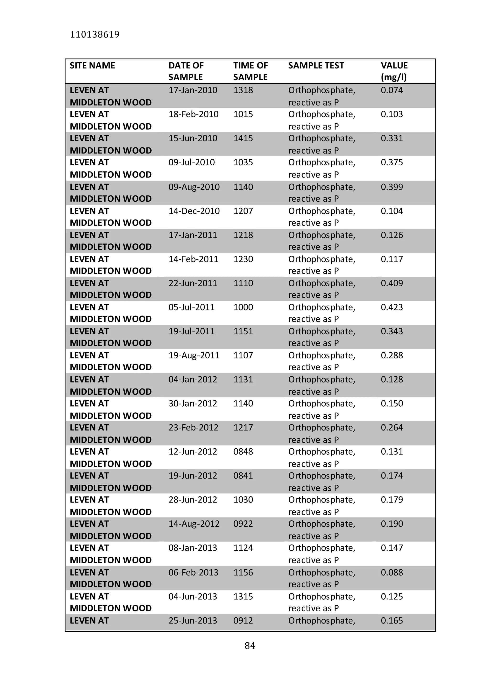
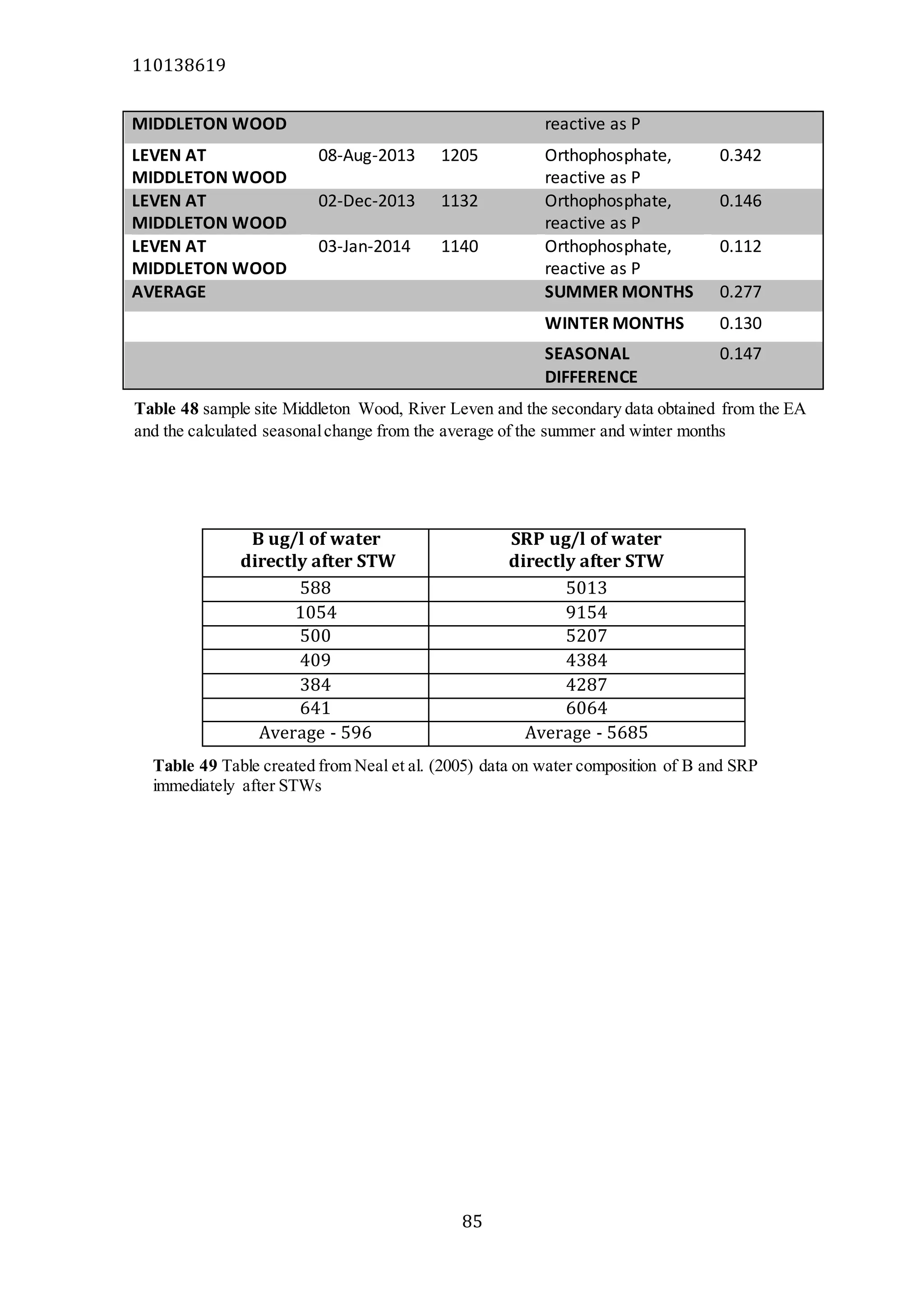
Boron:Morethan just a marker
for sewage effluent
Martyn Tattersall
110138619
1
Abstract
18 sites across 11 rivers in the Northumbria River Basin were sampled and analysed for
soluble reactive phosphorus (SRP) and boron (B) so that the variables could be used to see
the interaction between SRP and B and the relationship between a soluble reactive
phosphate and boron ratio (SRP:B) and a seasonal change of SRP (SC_SRP) method of
determining sources of P. The data suggests that there is a statistically significant positive
relationship between the variables B and SRP; SRP and SC_SRP and a statistically
significant negative relationship between the variables B and distance from nearest city
(DNC); SRP and DNC. The relationship between SRP and SC_SRP shows that sites with
SC_SRP values closest to the even contribution figure (ECF) show the smallest SRP
values. An increase in the magnitude of SC_SRP showed an increase in SRP particularly
when SC_SRP is positive. Regression analysis suggests that there is a moderate correlation
between SRP:B and SC_SRP that is significant at P = 0.05. The model produces
predictions of dominant P source that agrees with both tests and outlines any sites that vary
away from the norm. The most promising method explored is by multiple regression
analysis of SRP;B and B in predicting SC_SRP values, there is a strong positive
correlation. Estimated SC_SRP (eSC_SRP) values produced from the regression equation
were correlated with actual SC_SRP values using spearman’s rho and found the
relationship to be statistically significant at P = 0.001. Alternative methods using export
coefficients are too complex for reliable predictions or are too basic and produce unreliable
predictions. This test is significant and meets Water Framework Directive (WFD)
requirements of being simple, quick and cost effective.
Key words: Soluble reactive phosphorus, Boron, Water Framework Directive, SC_SRP,
Eutrophication, Management strategies.
Word Count: 9737
110138619
2
CONTENTS Page Number
Title page
Declaration
Abstract……………………………………………………………………………1
Contents…………………………………………………………………………...2 - 4
Abbreviations……………………………………………………………………..5
Figures…………………………………………………………………………….6
Tables……………………………………………………………………………..7-8
Acknowledgments……………………………………………………………......9
1. INTRODUCTION………………………………………………………….....10-12
1.1 General……………………………………………………………………….10-11
1.2 Aims and Objectives………………………………………………………....11-12
1.3 Hypotheses…………………………………………………………………...12
2. LITERATURE REVIEW…………………………………………………......13-22
2.1 Phosphorus in England’s Surface Waters………………………………...….13
2.2 The European Water Framework Directive……………………………...…..14-15
2.3 Phosphorus and Eutrophication………………………………………...…....15-17
2.4 Sources of Phosphorus……………………………………………………….18-19
2.5 Methods of Phosphorus Source Determination………………………...……19-22
2.5.1 Export Coefficient Model…………………………………….……20-21
2.5.2 Boron as a Marker for Sewage Effluent……………………….…..21-22
2.5.3 Seasonal Variability of Phosphorus…………………………….….22
3. METHODOLOGY…………………………………………………………....23-39
110138619
3
3.1 Site Description……………………………………………………………..23-24
3.2 Collection of Data…………………………………………………………..25
3.3 Sampling…………………………………………………………………….26-37
3.4 Chemical Analysis – Boron…………………………………………………38
3.5 Nutrient Analysis – Soluble Reactive Phosphorus………………………….38
3.6 GQA Standards……………………………………………………………...39
3.7 Result Analysis……………………………………………………………...39
4. RESULTS…………………………………………………………………….40-59
4.1 General Results……………………………………………………………...40
4.2 Soluble Reactive Phosphate Results………………………………...………41-42
4.3 Boron Results………………………………………………………………..42-43
4.4 Variables Statistics…………………………………………………………..44-50
4.4.1 B and SRP…………………………………………………………44-45
4.4.2 SRP and SC_SRP………………………………………………….45-47
4.4.3 B and Urban Land Use (DNC)……………………………...….....47-48
4.4.4 SRP and Urban Land Use (DNC)…………………………...…….48-49
4.4.5 Multiple Regression of SRP with B and DNC……………...…….50
4.5 Method Statistics……………………………………………………...….....51-59
4.5.1 SRP:B and SC_SRP……………………………..........................51-52.
4.5.2 B and SC_SRP………………………………..............................53-55
4.5.3 Multiple Regression of SC_SRP with SRP:B and B………….....55-56
4.5.4 eSC_SRP and SC_SRP……………………………………..........57-59
5. DISSCUSSION……………………………………………………………....60-67
5.1 Variable Statistics…………………………………………………………...60-65
5.1.1 B and SRP………………………………………………………....60-62
5.1.2 SRP and SC_SRP………………………………………………....62-63
5.1.3 B and SRP Response to Urban Land Use (DNC)……………..….64-65
5.2 Method Analysis………………………………………………………...…..65-67
110138619
4
5.2.1 SRP:B and SC_SRP………………………………………………..65-66
5.2.2 B and SC_SRP……………………………………………………..66
5.2.3 Multiple Regression of SC_SRP with SRP:B and B……………....67
6. CONCLUSION………………………………………………………………..67-68
7. LIMITATIONS AND IMPROVEMENTS……………………………………68
8. APPENDICES………………………………………………………………...69-87
8.1 Primary Data…………………………………………………………………69
8.2 Secondary Data………………………………………………………………70-85
8.3 Other…………………………………………………………………………86-87
Fieldwork Risk Assessment Form…………………………………………........88-92
Laboratory use form
9. BIBLIOGRAPHY …………………………………….…………………..…93-99
110138619
5
Abbreviations
AES Atomic Emission Spectrometer
B Boron
CIEEM Chartered Institute of Ecology and Environmental Management
DNC Distance from Nearest City
EA Environment Agency
ECF Even Contribution Figure
eSC_SRP Estimated Seasonal Change of Soluble Reactive Phosphorus
EU European Union
ICP – MS Inductively Coupled Plasma Mass Spectrometer
ICP – OES Inductively Coupled Plasma Optical Emission Spectrometry
LOIS Land – Ocean Interaction Study
NRBD Northumbria River Basin District
P Phosphorus
SC_SRP Seasonal Change of Soluble Reactive Phosphorus
SRP Soluble Reactive Phosphorus
SRP:B Soluble Reactive Phosphorus to Boron Ratio
STWs Sewage Treatment Works
UK United Kingdom
u/s Upstream
WFD Water Framework Directive
110138619
6
Figures
Figure Description Pg.
1 The proportion of waters in the NRBD in good condition. 10
2 Target phosphorus concentrations for river in England and Wales with
suggested applications for the type of river
16
3 Export coefficient figures for different land uses to be used in P source
determination methods
20
4 A map of Northumbria outlining the four regions within the district, the change
from rural in the west to urban in the east and the major rivers in the NRBD
24
5 A site map with corresponding site numbers. Shows the general relief of the
catchment area.
27
6 A site map with corresponding site numbers. Illustrates the rural and urban land
use areas
28
7 Site 1. Pauperhaugh, River Coquet 29
8 Site 2. Clap Shaw, River Derwent 29
9 Site 3. Middleton Wood, River Leven 30
10 Site 4a. Jesmond Dene, River Ouseburn 30
11 Site 4b. Three Mile Bridge, River Ouseburn 31
12 Site 5. South Park Darlington, River Skerne 31
13 Site 6a. u/s Birtley STW, River Team 32
14 Site 6b. Lamesley, River Team 32
15 Site 7a. Dinsdale, River Tees 33
16 Site 7b. Dent Bank, River Tees 33
17 Site 8. Wark, River North Tyne 34
18 Site 9. Alston, River South Tyne 34
19 Site 10a. How Burn, River Wansbeck 35
20 Site 10b. Mitford, River Wansbeck 35
21 Site 11a. Bishop Auckland, River Wear 36
22 Site 11b. Cocken Bridge, River Wear 36
23 Site 11c. Stanhope, River Wear 37
24 Site 11d. Shincliffe Bridge, River Wear 37
25 The graph of the linear regression model between SRP (mg/l) and B (mg/l) 45
26 The graph of the linear regression model between SC_SRP (mg/l) and SRP
(mg/l)
47
27 The graphs from exponential curve estimation between B (mg/l) and DNC (km)
and between SRP (mg/l) and DNC (km)
49
28 The graphs from exponential curve estimation between B (mg/l) and DNC (km)
and between SRP (mg/l) and DNC (km)
49
29 The graph from linear regression between SC_SRP (mg/l) and SRP:B 52
30 The graph from linear and cubic regression between B (mg/l) and SC_SRP
(mg/l)
55
31 The graph from linear regression between eSC_SRP (mg/l) and SC_SRP (mg/l) 59
32 A stacked histogram showing the relationship between SRP and B as the
volume of sewage effluent increases
60
33 A map of past coal mining areas in the NRBD. Represented by the semi-
transparent area within the black margins
62
34 Diagram and equations to illustrate how changes in concentration vary in
magnitude depending on the initial concentration
63
35 4 graphs to show the concentrations of TP when point source contributes (a) 0 –
25% (b) 25- 50 % (c) 50 – 75% and (d) 75-100% of the phosphorus load
87
110138619
7
Tables
Table Description Pg.
1 A table of sampled rivers and the sites along them 26
2 GQA classification table for phosphates 39
3 Table of sampling sites and their DNC figures 40
4 Table of sampling sites and their SRP concentrations 41
5 Table of sampling sites and their SC_SRP values 42
6 Table of sampling sites and their B concentrations 43
7 Model summary of SRP and B 44
8 ANOVA output of SRP and B 44
9 Model summary of SC_SRP and SRP 46
10 ANOVA output of SC_SRP and SRP 46
11 Model summary of B and DNC 47
12 ANOVA output of B and DNC 48
13 Model summary of SRP and DNC 48
14 ANOVA output of SRP and DNC 48
15 Model summary of SRP and the variables B and DNC 50
16 ANOVA output of SRP and the variables B and DNC 50
17 Coefficients output of SRP and the variables B and DNC 50
18 Model summary of SRP:B and SC_SRP 51
19 ANOVA output of SRP:B and SC_SRP 51
20 Coefficients output of SRP:B and SC_SRP 51
21 Model summary of B and SC_SRP 53
22 ANOVA output of B and SC_SRP 53
23 Model summary of B and SC_SRP 54
24 ANOVA output of B and SC_SRP 54
25 Model summary of SC_SRP and the variables SRP:B and B 56
26 ANOVA output of SC_SRP and the variables SRP:B and B 56
27 Coefficients output of SC_SRP and the variables SRP:B and B 56
28 Sample sites and their recorded SC_SRP values and their eSC_SRP values 57
29 Model summary of eSC_SRP and SC_SRP 58
30 ANOVA output of eSC_SRP and SC_SRP 58
31 Correlations output from Spearman’s rho correlation analysis between
eSC_SRP and SC_SRP
59
32 Sample sites and all their data for the variables: B, SRP,P,SC_SRP and DNC 69
33 Shincliffe Bridge, River Wear and the secondary data obtained from the EA 70
34 Cocken Bridge, River Wear and the secondary data obtained from the EA 71
35 Bishop Auckland, River Wear and the secondary data obtained from the EA 2
36 Stanhope, River Wear and the secondary data obtained from the EA 73
37 Alston, River S Tyne and sample site Wark,River N Tyne and the secondary
data obtained from the EA
74
38 Mitford, River Wansbeck and sample site u/s How Burn confluence, River
Wansbeck and the secondary data obtained from the EA
75
39 Pauperhaugh, River Coquet and the secondary data obtained from the EA 76
40 Clap Shaw, River Derwent and the secondary data obtained from the EA 76-77
41 u/s Birtley STWs, River Team and the secondary data obtained from the EA 77
110138619
8
42 Lamesley, River Team and the secondary data obtained from the EA 78-79
43 Dent Bank, River Tees and the secondary data obtained from the EA 79
44 Dinsdale, River Tees and the secondary data obtained from the EA 80
45 Jesmond Dene,River Ouseburn and the secondary data obtained from the EA 81
46 Three Mile Bridge, River Ouseburn and the secondary data obtained from the
EA
82
47 South Park Darlington, River Skerne and the secondary data obtained from the
EA
83
48 Middleton Wood, River Leven and the secondary data obtained from the EA 84-85
49 Data on water composition of B and SRP immediately after STWs 85
50 Key pressures being applied on phosphorus control in rivers 86
51 Summary of the NRBD sectors identified that are preventing good status to be
reached
87
110138619
9
Acknowledgments
I would like to thank many people for making this dissertation possible.
I wish to thank Emma Pearson and Simon Drew for allowing me to use the laboratory and
its analysis equipment. I wish to thank Andy Large for giving me guidance and keeping me
calm at particular times of worry.
Thanks goes to Doug Meynell of Lanes PLC for making the connection with Northumbria
Water and to Lanes Group plc for funding the boron analysis.
Thanks go to the Northumbria Water laboratories for analysing the boron.
Final thanks go to my family for continuous support.
110138619
10
1. Introduction
1.1 General
The Water Frame Directive (WFD) was officially published in 2000 by the EU with an aim
to achieve good water status in all European waters by 2015 (Hering et al., 2010; Mostert,
2003). In the directive phosphorus is targeted in particular because of its relationship with
eutrophication as the key limiting nutrient (EA, 2012; Hilton et al., 2006; Jarvie et al.,
2006). Eutrophication of waters requires a lot of attention as it causes adverse effects on
water use and its social benefits (EA, 1012) as well as the detrimental effect it can have on
river ecology health (Hilton et al., 2006). In Northumbria the location of this study, rivers
suffer from poor ecology more than any other surface water body (figure 1) outlining the
importance of river management strategies with respect to this study.
The WFD requires a technique that is simple, reliable and cost effective so that mitigation
strategies can be put in place to improve the rivers in time for the 2015 deadline (EA,
2000; Hilton et al., 2002; May et al., 2001; Neal et al., 2008). Methods to improve to
phosphorus levels in rivers include an increase in tertiary treatment in STWs for rivers
Figure 1 The proportion of waters in the NRBD in good condition. From EA (2013)
110138619
11
affected by point source inputs, or riparian buffer strips and improved farming practices
(Bowes et al., 2008). Management strategies can only be successfully administered when
the relative contributions of point and diffuse sources of phosphorus is calculated (Bowes
et al., 2008).
Research into finding a method that meets the WFD requirements has seen the increase in
studies using boron as a marker of sewage effluent to be used in conjunction with
phosphorus source determination methods (Jarvie et al., 2002; Jarvie et al., 2006; Neal et
al., 2010). It was Neal et al. (1998) that proposed the development of techniques using
boron as an indicator is a big step towards the development of management strategies
before the WFD was even installed. However this project aims to move past the
restrictions of boron as a marker for sewage effluent. Instead it intends to offer an
alternative approach to determining the sources of phosphorus with boron at the heart of
the investigation.
1.2 Aims and objectives
Aims - To produce a simple but effective method of determining the dominant source
of phosphorus for rivers, using boron based methods in relation to the
seasonal variation of phosphorus method.
To confirm findings in previous studies of the relationship between soluble
reactive phosphorus and boron, and that B is a useful marker of sewage
effluent.
Objectives – Develop a suitable methodology for collection and detection of appropriate
water characteristics at sites that will support the study, through literature and
Environment Agency (EA) water quality sites.
Choose suitable techniques to analyse the water samples in the laboratory that
will best support the aims of the study.
Use suitable statistical techniques to assess the relationship between boron
and soluble reactive phosphorus to accept or reject the null hypothesis.
110138619
12
Use suitable statistical techniques to test the effectiveness of the study
techniques against an agreed upon selected technique for determining
dominant phosphorus source from literature, with an aim to accept or reject
the null hypothesis.
1.3 Hypotheses
1. H0 = There is no statistically significant relationship between soluble reactive
phosphorus and boron.
2. H0 = There is no statistically significant relationship between the ratio of soluble
reactive phosphorus with boron and the seasonal variability of soluble reactive
phosphorus.
110138619
13
2. Literature Review
2.1 Phosphorus in England’s surface waters
The EA recognises that phosphorus is the most common failing WFD element in England.
There have been significant reductions in phosphorus post 1990 with the major reductions
in STW loading (EA, 2013). The percentage of rivers with high phosphorus levels has
fallen from 69% in 1990 to a current 45% (EA, 2013). However, of these 45%, half are
more than 2.5 times over the ‘good status’ level and a further quarter of rivers are more
than 5 times over the level (EA, 2013). The poor phosphorus levels have the biggest
impact on England plant and animal communities, and the natural processes, structure and
function of ecosystems in the UK.
In England the main source of river phosphorus is from sewage effluent. The EA (2013)
estimates that it contributes 60-80% of the total phosphorus and that the agricultural sector
adds 25% of the total phosphorus found in England’s waters. The relative proportion of the
two depends on the catchment land use. Heavily urban river basins like the Thames district
produces enough domestic waste to fill 900 Olympic sized swimming pools every day
(EA, 2013), whereas, an intense agricultural basin like the Anglian River Basin with a
population of only 7.1 million will have less impact on river phosphorus from sewage
effluent and more from agricultural practice (EA, 2013). On average, detergents account
for 16% of the total phosphorus added by sewage, with food and drink only making up 6-
10% of sewage (EA, 2013). Phosphorus stripping of the sewage is unfortunately not
enough to keep the river phosphorus levels below the ‘good status’ standard as nationally
the EA (2013) estimates that there are 100,000 misconnections in the English sewer works.
The misconnections take foul waters containing high phosphorus loads and export them
into freshwater systems instead of exporting them to be treated. During times of heavy
precipitation foul water sewers can also fail and overflow into safe water sewers and again
be exported to freshwater systems increasing the phosphorus load. England also has 1500
km2 of road surfaces that produce urban run off at times of high precipitation, dumping
contaminants and phosphorus directly into the rivers (EA, 2013). Phosphorus is the main
issue for freshwater river systems in England and this is reflected in the WFD.
110138619
14
2.2 The European Water Framework Directive (WFD)
The WFD was adopted in 2000 by the EU in an attempt to unite the water policies and
regulations of the European nations, outlining the general rule that humans can take
advantage of water resources as long as the ecology of the system is not significantly
harmed (Dworak et al., 2005). The establishment of the WFD has provided the most
significant development towards the improvement of surface waters in Europe (Hilton et
al., 2006). Mostert (p.523, 2003) outlines that the specific aims of the directive are:
1. To reduce pollution of surface and groundwaters by reducing inputs of selected and
hazardous priority substances.
2. To prevent further deterioration of water bodies.
3. To promote sustainable water use.
4. To reduces the effects of extreme water conditions; flooding and droughts.
The overall objective was to achieve a ‘good water status’ by 2015 (Mostert, 2003). To
achieve the aims a management strategy was put in place. The EU enforced a change in the
way that water quality was viewed, from an individual chemical assessment of the river to
a wider concept of the river basin ecology (Bateman et al., 2006). The individual basins
could be assigned an authority and produce an individual management plan to take the
region from identifying the health status to identifying the success or failure of the
management scheme in 2015 (Allan et al., 2006; Mostert, 2003).
To support the aims of management schemes it required the establishment of monitoring
programmes divided into three categories (Dworak et al., 2005):
 Surveillance monitoring- to assess the long term changes in river health
 Operational monitoring- to be used as an extra measure for those rivers at risk of
not meeting the ‘good status’ by 2015.
 Investigative monitoring- to be used when the standards are not met for an
unexplained reason.
For each monitoring type an assessment of biological qualities, chemical qualities and
hydromorphological qualities are produced (Allan et al., 2006). Operational monitoring has
110138619
15
been the main focus by the EU nations with 17 of the 25 states favouring operational
monitoring over surveillance monitoring (Hering et al., 2010) indicating that the main
efforts are focused primarily on the restoration side of the WFD. With the increase of
monitoring there is a need to improve the efficiency of monitoring. Monitoring tools must
advance to provide the large amount of data required, at a low cost and within a suitable
time frame (Allan et al., 2006). The technical advancement could involve developing tools
that record river data on site (Allan et al., 2006) however such tools may be able to record
levels of phosphorus but will be unable to determine the source without further
information. The aim of this work could provide a suitable alternative for this situation
with particular beneficial qualities for investigative monitoring. Current methods that have
been developed are criticised for being too complex in their aim for perfection (Hering et
al., 2010) instead of providing a quick simple method to show the appropriate direction
that measures should be taken like this paper aims to do.
Although the methods for implementing the WFD are still being decided upon, the WFD
has started the process of standardised European water enforcements including the way
that river systems are approached, monitored and managed (Hering et al., 2010). The
deadline of 2015 is ambitious but it has made EU nations put time and effort into the
process that otherwise wouldn’t have happened (Jones & Schmitz, 2009). Without the
increase in river monitoring the secondary data for this paper would not be available, or
available for other studies.
2.3 Phosphorus and eutrophication
Phosphorus is a high priority substance addressed in the WFD because of its association
with eutrophication and the harmful effects like nuisance phytoplankton it brings (Jarvie et
al., 2006). Phosphorus is an unsustainable rock that is mined for fertilisers, detergents and
other products (EA, 2002). Phosphorus can take different forms within the water column
varying between organic or inorganic and particulate or dissolved (Jarvie et al., 2005).
However the most abundant form in rivers is SRP averaging 67% of the total phosphorus
(Jarvie et al., 2006). The most eutrophic plant species take up SRP from the water column
suggesting it is the main form to focus on in studies regarding eutrophication and nutrients
(Hilton et al., 2006)
110138619
16
Eutrophication has been recognised as an international concern since the 1990s (EA, 2012)
and has been extensively linked with phosphorus as the key limiting nutrient in studies
(EA, 2012; Hilton et al., 2006; Jarvie et al., 2005; Jarvie et al., 2006; Mainstone and Parr,
2002). SRP was even used by the EA (2000) to set the guidelines for good health for
different river types (figure 2). Studies taken by the EA (2012 and 2002) showed that river
integrity and phosphorus were negatively correlated as well as a strong positive correlation
between planktonic algae and phosphorus enrichment in large rivers.
Eutrophication is rarely a natural phenomenon but with anthropogenic influences it can
cause the shift from macrophytes to algae dominance, stimulate the excessive growth of
the algae, lower the dissolved oxygen content of the water column, promote blue green
cyanobacteria growth and increase the turbidity of the water (Hilton et al., 2006). 50% of
failing lakes and 60% of failing rivers in the US are due to eutrophication; however on
average the amount of suspended algae in lakes is significantly higher than in rivers
(Smith, 2003). Smith (2003) suggests that this is because of the velocity of the flow but in
Young et al. (1999) study they found that the relationship between flow and suspended
algae was not significantly connected and went further to find that phosphorus wasn’t the
limiting factor as it was readily available. The limiting factor of eutrophication may be due
to environmental factors of light intensity, turbidity, temperature or the availability of other
important nutrients (Mainstone and Parr, 2002).
Throughout the extensive studies on river eutrophication it is the new paradigm suggested
by Hilton et al. (2006) that appears the most likely: it is not the velocity of the flow that is
important but the duration. Reynolds (1984) suggests that it takes two days for algae cells
to replicate so in the context of a lake, algae blooms will be a possibility when retention
Figure 2 Target phosphorus concentrations for river in England and Wales with suggested
applications for the type of river. From EA (2000)
110138619
17
time is longer than 4 days. However as inoculum of suspended algae is minimal at the
source of the river the duration time must be greater than 4 days, promoting benthic algae
growth in smaller rivers as opposed to phytoplankton (Hilton et al., 2006). Conversely,
with rivers that have a long duration time due to their large lengths and depths, there is
time for sufficient replications of suspended algae to promote growth and make it the
dominant plant species. In general, phytoplanktonic species will increase with distance
downstream (Hilton et al., 2006). With the similarities between retention time and duration
time the eutrophic processes of lakes and some rivers could be looked at in a similar way
(Smith, 2003) proven by Reynolds et al. (1998) when a minor adaptation of the PROTECH
lake model was used to predict potamoplankton on the River Thames.
The undesirable effects of eutrophication are most prominent during the low summer flows
(Jarvie et al., 2006). These outcomes can be separated into environmental effects and
social effects. With increases in turbidity and phytoplankton the water column can
potentially become anoxic and cause mass fish deaths (Withers and Jarvie, 2008). If
eutrophic blue-green cyanobacteria are formed it can release deadly toxins again killing
fish and reducing biodiversity (Hilton et al., 2006).
Socially eutrophication disturbs angling, conservation interests, navigation and, because of
its unattractive aesthetics, it affects tourism and water front property prices (EA, 2012).
Further economic consequences include algae growth within reservoirs increasing the cost
of water cleansing to achieve drinking water standards and increasing the risk of flooding
by the stimulated growth of excessive rooted plants (Hilton et al., 2006).
Hilton et al. (2006) estimate that it costs £100 million per year to address the effects of
eutrophication on society. With the WFD in place it is vitally important that it is followed
through to reduce these costs. Eutrophication is clearly an expensive issue highlighting the
importance of this paper.
110138619
18
2.4 Sources of phosphorus
Sources of phosphorus can be natural or anthropogenic. Natural sources can be from soil
weathering, riparian inputs, fish migration and bank erosion (Walling et al., 2008; Withers
and Jarvie, 2008). Furthermore, atmospheric sources of phosphorus in precipitation are
small only reaching 10 mg/l (Wood et al., 2005). Natural sources provide small amounts of
phosphorus and in the non-bioavailable form of particulates so it can be eliminated as a
threat to stream health (Withers and Jarvie, 2008). Wood et al. (2005) proved this by
finding no evidence to support bank erosion inputs of phosphorus on the River Taw.
Anthropogenic sources can be divided into three categories: point, intermediate and diffuse
sources (Neal et al., 2005). Sewage treatment works (STWs) are the main point sources.
STWs discharge effluent rich in detergents, food and phosphorus from lead dosing directly
into water courses (EA, 2012; Neal et al., 2005). SRP is the dominant form of phosphorus
emitted into the rivers from STWs, providing immediate availability for plant use
(Mainstone and Parr, 2002). A combination of continuous SRP inputs throughout the year
and minimum dilution at low flows in summer make a high risk of eutrophication (Bowes
et al., 2005). The concentration of phosphorus in sewage effluent depends on the scale of
treatment the STWs apply, the size of the population it provides for and the industrial
activity within the sewered area (Withers and Jarvie, 2008). After primary, secondary and
tertiary treatment the average phosphorus concentration lies between 1 and 20 mg/l
(Withers and Jarvie, 2008).
Future population growth will exacerbate the risk of eutrophication with the increase in
sewage load, particularly in areas already exceeding phosphorus WFD standards (EA,
2002). The WFD estimates that there will be 650 STWs with tertiary treatment serving 24
million people by 2015 (EA, 2002).
Intermediate sources include run-off from urban land uses like roads and cities, and
phosphorus from septic tanks (Jarvie et al. 2006). The majority of UK rural areas rely on
septic tanks as their sewage removal mechanism (Wood et al., 2005). Septic tanks
discharge onto areas of low soil saturation, however in heavy rainfall events this can be
washed into river systems as a source of phosphorus (Neal et al., 2008). Furthermore areas
relying on older septic tanks may release their waste directly into rivers, or have an
110138619
19
irregular and large release of effluent leading to high soil and river phosphorus
concentrations (Withers and Jarvie, 2008).
Urban run-off mobilises sources of phosphorus such as dead vegetation, litter, industrial
matter and disturbed soils during high precipitation events. Although the process is
intermittent it contributes a rapid supply of phosphorus directly into the river course (Neal
et al., 2005).
The WFD has caused an increase in tertiary treatment of sewage. Jarvie et al. (2006)
estimated that agriculture contributed to 50% of the annual river phosphorus in the UK. It
is the application and removal of fertilizers from agricultural lands that defines it as a
diffuse source (Neal et al., 2005). The addition of phosphorus from diffuse sources is very
seasonal (Mainstone and Parr, 2002). Cooper et al. (2002) suggested that for the Thames
catchment 66-84% of the annual diffuse phosphorus load was transported during the winter
months. The majority of the load is delivered as non-bioavailable particulates (Mainstone
and Parr, 2002) so may not be the main contributor to eutrophic conditions unlike STWs.
The quantification of phosphorus loads from the highly variable catchment sources is
difficult and impossible to be 100% accurate (Bowes et al., 2005). However it is possible
to identify the key contributing source and reduce risks arising from phosphorus
enrichment.
2.5 Methods of phosphorus source determination
Producing methods to assess the relative contributions of phosphorus to rivers has become
increasingly important since the introduction of the WFD (Bowes et al., 2008; EA, 2000;
Hilton et al., 2002; Neal et al., 2008). The required method needs to be simple, low cost
and accurate enough to assess which source needs to be addressed (Hilton et al., 2002). It
is the development of these methods that will ensure a sustainable, affordable success of
the WFD goals (Jarvie et al., 2002).
110138619
20
2.5.1 Export coefficient model
The most common method being developed is the export coefficient model, pioneered by
Johnes (1996) before the instalment of the WFD. Since Johnes (1996), the method has
been studied and improved to attempt to reach WFD standards. In 2001 studies (May et al.;
Wang) used aerial imagery to measure the extent of different land uses in the catchment
and assigned particular coefficients (figure 3) for their contribution of phosphorus to the
river. The export coefficients were based on an annual study of run offs or from scaling up
results from small tests on each land use (Hilton et al., 2002). Hilton et al. (2002)
attempted to reduce the complexity by assigning predesigned uncalibrated coefficients
based on generic land uses. The relative contribution of diffuse sources was calculated
based on the area of land uses upstream of STWs and urban influence and point sources
downstream (Hilton et al., 2002). Bennion et al. (2005) progressed the method further by
applying export coefficients to point loading by STWs. The volume of phosphorus loaded
was estimated by a population in the catchment coefficient (Wood et al., 2005).
There are a large number of water quality models but they do not meet the requirements of
the WFD because they are too complex, require too much data, are time consuming or are
unreliable (EA, 2000). For the UK the main priority is estimating the influence of STWs.
Figure 3 Export coefficient figures for different land uses to be used in P source determination
methods. From May et al. (2001)
110138619
21
Methods that require data on direct sewage effluent are rare because of the inaccurate or
sparse data collected on effluent composition (Boorman, 2003; Wood et al., 2005).
Producing export coefficients for STWs like in the Bennion et al. study (2005) does not
distinguish between houses that are served by STWs and those that rely on septic tanks
(Wood et al., 2005), it does not account for varying levels of effluent treatment from STWs
or for the transfer of sewage from one catchment into another (Wood et al., 2005). Without
these complications there is also no universal figure for phosphorus levels in sewage
effluent. In the original Johnes (1996) study a coefficient of secondary treated effluent was
0.38 kgP/capita/y whereas in the Carvalho et al. (2003) study the value ranged from 0.14-
1.55 kgP/capita/y.
To produce accurate models to predict diffuse inputs it requires even larger amounts of
data (Bowes et al., 2008; Hilton et al., 2002; Wang, 2001): fertiliser use, livestock
numbers, stock headage, type of agriculture, meteorology and several years of water
monitoring data to establish a calibrated set of coefficients. Data that is rare and requires
years of research. In the Hilton et al. (2002) study the uncalibrated export coefficients
could not be reliable as they may not have been appropriate for the studied catchment
(Bowes et al., 2008) indicating that the method is even more complicated to try
simplifying. Most models are not acceptable for regular monitoring on a lot of catchment
sites (EA, 2000).
2.5.2 Boron as a marker of sewage effluent
The use of boron in aquatic investigations was pioneered by Neal et al. (1998) in the Land-
Ocean Interaction Study (LOIS) (Jarvie et al., 2002). Boron is an element that is present in
aquatic ecosystems from both natural and anthropogenic sources (Fox et al., 2000).
Sewage effluent is rich in boron as it is made up of boron-containing substances (Jarvie et
al., 2002; Jarvie et al., 2006; Neal et al., 1998; Neal et al., 2010): detergents, washing
powders, soaps and cleaning products. In water bodies boron is found in the stable
unreactive form borate because of its high affinity for oxygen (Jarvie et al., 2002; Neal et
al., 1998; Wyness et al., 2003). The chemically unreactive borate was identified by the
LOIS studies as a useful marker for sewage because of its stable form in water and its
strong correlation with sewage phosphorus (Jarvie et al., 2006; Neal et al., 1998; Neal et
110138619
22
al., 2005). These characteristics could prove useful in methods to determine sources and
impacts of phosphorus (Neal et al., 2010).
Natural sources of boron from weathered igneous rocks and leaching of salt deposits can
produce a background source that need to be taken into account when using boron as an
effluent marker (Jarvie et al., 2006; Neal et al., 1998; Neal et al., 2005). With this study the
background reading is minimal (<10 ug/l) because of the areas predominant sedimentary
geology and minimal saline deposits (Neal et al., 1998).
Neal et al. (1998) believed that the use of boron in studies of this kind is a key step in
improving management strategies for water quality. Boron has been used as an indicator or
facilitator in studies on hydrodynamic behaviour of STWs (Fox et al., 2000), sewage and
other river inputs (Jarvie et al., 2002) and the impact of tertiary treatment on sewage
effluent (Neal et al., 2000). In studies that have limited access to sewage effluent records
or require a more reliable source of data than export coefficients, boron as a tracer is a
sensible option (Neal et al., 1998).
2.5.3 Seasonal variability of phosphorus
With every model associated with phosphorus inputs there has been one general
conclusion relating the seasonal variability of phosphorus with its appropriate source.
Rivers with predominantly point source inputs of phosphorus experience the highest
concentrations during the summer months when dilution is at its lowest whereas rivers that
are predominantly diffuse source influenced have the highest concentrations in the winter
months when rainfall and flow are highest (Bowes et al., 2005; Bowes et al., 2008; Cooper
et al., 2002; Jarvie et al., 2002; Jarvie et al., 2006; May et al., 2001; Neal et al., 1998;
Nishikoori, 2011; Wood et al., 2005).
There is no unified approach of monitoring source inputs of phosphorus in to rivers
(Wyness et al., 2003) but the development of methods is essential in the aim to control
eutrophication (May et al., 2001). However we know that using estimates from catchment
uses will not be as reliable as actual river monitoring (Bowes et al., 2008). Boron could
play a key role in future methods, and this study aims to use it in conjunction with the only
agreed upon method of seasonal variability.
110138619
23
3. Methodology
3.1 Site Description
The rivers being used for testing whether B can be used to infer STW inputs are located in
the Northumbria River Basin District (NRBD). The NRBD covers 9029 km2 and is home
to 2.5 million people (EA, 2013). The area is comprised of Northumberland, County
Durham, parts of North Yorkshire and Cumbria. Over the large area of land there is a great
variation in land uses and land types: industrial, urban regions, hills and valleys in the
Northumberland National Park and Pennine regions and coastal features along the east
side. 67% of the land is used for farming or forestry and only 693km2 of the land is urban
(EA, 2007). Towards the west, away from the coast and urban cities the NRBD has a
predominantly rural setting with heather moorland coverage. In the north and west areas
with higher reliefs there is extensive sheep grazing. As you move further east and south to
the lower flatter lands the land use changes to arable or mixed farming practices. Mining
and quarrying were once wide spread in the district however industry and manufacturing
still remains important in the industrial cities to the east. The main industries are chemical,
petrochemical, metal sectors and transport sectors (EA, 2013).
The human influence over the land produces a variety of different methods that can
influence or harm freshwater ecosystems. Out of the 362 rivers, 42% are deemed to be in
moderate condition (EA, 2007). 17% of the NRBD freshwater failures are due to sewage
inputs from industry, 16% from rural pollution and 6% from urban sewage system failure
(EA, 2013). In 2015 the government are aiming to improve the sewer networks to reduce
failing during high rainfall, if B can be used to infer P inputs selection of areas to improve
can be identified better and quicker. Furthermore, with a predominantly Carboniferous and
Cretaceous sedimentary bedrock the NRBD has low background B concentration making it
the perfect site to test for relationship between B and water quality (Neal et al., 1998).
110138619
24
Figure 4 A map of Northumbria outlining the four regions within the district, the change from
rural in the west to urban in the east and the major rivers in the NRBD. From EA (2013)
110138619
25
3.2 Collection of data
To assess whether a B:P ratio could be used as a method of river nutrient analysis it
requires both primary and secondary data. Secondary data was supplied by previous
samples collected by the Environment Agency at the sites specific to the investigation
(tables 33-48). The samples were tested for orthophosphates. The data provided was
reduced to leave only data that met the required categories: data post 01/01/1995, data
taken from the summer months of June, July and August, data taken from the early winter
months of December and January. The data restrictions were put in place to avoid using
out dated information and to provide the seasonal change in orthophosphates used an
analogue for point source determination method comparisons.
Rivers and sites for primary data were selected by following principles needed to assess
the effectiveness of the proposed method. The rivers required:
1. A broad range of phosphate input methods.
2. A large influence on the overall freshwater health of the NRBD.
3. A frequent monitoring programme.
A general rule that as distance downstream increases, urban land use increases and there is
a larger point source input of phosphates was used to help select sites along the rivers to
meet the criteria of the first principle. Using the secondary data provided by the
Environment Agency in conjunction with google maps appropriate sites were selected
based on the 3 principles. Time restraints and vehicle accessibility also played a part in
finalising the sites.
The primary data collection period took 3 days from 27/11/2013-29/11/2013. This was a
period of constant dry weather which had followed a week of rainfall, allowing the
assumption that the samples were taken under the same conditions. When applying the
‘dilution and drainage’ theory, the data collected would show relatively low
orthophosphate levels in areas affected by point source inputs such as STWs and high
orthophosphate levels in diffuse source affected areas.
110138619
26
3.3 Sampling
Nineteen sites were chosen for sampling, spanning across eleven rivers in the North East
region of England (table 1). An on-site judgemental approach was taken to decide the
specific sample site. The specific site was selected by: taking time restraints into account,
safety precautions with the relatively high flows, river accessibility and avoiding static or
slow moving sites at the river’s edge as this allows more time for nutrient recycling and
use (Withers and Jarvie, 2008). At each site two 250ml plastic bottle grab samples were
collected, removing all air bubbles from the sample. The samples were placed into dark
storage to avoid adsorption and were put into below 4oC refrigeration at the first
opportunity. Analysis of the water samples was done within a week to keep holding times
to a minimum.
Site number River Location
1 Coquet Pauperhaugh
2 Derwent Clap Shaw
3 Leven Middleton Wood
4a Ouseburn Jesmond Dene
4b Ouseburn Three Mile Bridge
5 Skerne South Park Darlington
6a Team u/s Birtley STW
6b Team Lamesley
7a Tees Dinsdale
7b Tees Dent Bank
8 North Tyne Wark
9 South Tyne Alston
10a Wansbeck u/s How Burn confluence
10b Wansbeck Mitford
11a Wear Bishop Auckland
11b Wear Cocken Bridge
11c Wear Stanhope
11d Wear Shincliffe Bridge
Table 1 A table of sampled rivers and the sites along them.
110138619
27
1
2
3
4a
4b
5
6a 6b
7a
7b
8
9
11a
11b
11c
10a
10a
11d
10a
10b
Figure 5 A site map with corresponding site numbers. Shows the general relief of the catchment
area.
110138619
28
1
10b
10a
8
4b
4a
6a
6b
2
9 11c
11d
11a
11b
7b
5
7a
3
Figure 6 A site map with corresponding site numbers. Illustrates the rural and urban land use
areas.
110138619
29
Figure 7 Site 1. Pauperhaugh, River Coquet
Figure 8 Site 2. Clap Shaw, River Derwent
110138619
30
Figure 9 Site 3. Middleton Wood, River Leven
Figure 10 Site 4a. Jesmond Dene, River Ouseburn
110138619
31
Figure 11 Site 4b. Three Mile Bridge, River Ouseburn
Figure 12 Site 5. South Park Darlington, River Skerne
110138619
32
Figure 13 Site 6a. u/s Birtley STW, River Team
Figure 14 Site 6b. Lamesley, River Team
110138619
33
Figure 15 Site 7a. Dinsdale, River Tees
Figure 16 Site 7b. Dent Bank, River Tees
110138619
34
Figure 17 Site 8. Wark, River North Tyne
Figure 18 Site 9. Alston, River South Tyne
110138619
35
Figure 19 Site 10a. How Burn, River Wansbeck
Figure 20 Site 10b. Mitford, River Wansbeck
110138619
36
Figure 21 Site 11a. Bishop Auckland, River Wear
Figure 22 Site 11b. Cocken Bridge, River Wear
110138619
37
Figure 23 Site 11c. Stanhope, River Wear
Figure 24 Site 11d. Shincliffe Bridge, River Wear
110138619
38
3.4 Chemical analysis - Boron
There are a few methods that can be used for boron determination; the main two being
spectrophotometric and plasma-source spectrometric approaches. The samples were taken
to Northumbrian Water Scientific Services and an ICP-MS method was used. A plasma-
source method was favoured over AES as it has a higher sensitivity and can detect lower
concentrations of B and favoured over time consuming nuclear methods (Sah and Brown,
1997). The ICP-MS method was preferred to ICP-OES for the same reasons.
ICP-MS used argon induced plasma for sample ionization. The different ions were
detected in the mass spectrometer and a mass number for B was produced. The data was
then calibrated using an internal standard of beryllium as it has the closest mass number to
B and it is simple and efficient (Sah and Brown, 1997). A B concentration was produced in
the form mgl-1.
3.5 Nutrient analysis - soluble reactive phosphates
A HACH Portable Spectrophotometer (DR/2400) was used to measure orthophosphates
using a PhosVer3 ascorbic acid method: determination limits 0.02-2.5 mgl-1 PO4
3-. The
orthophosphate reacts with molybdate to form a phosphate-molybdate complex. The
ascorbic acid then reduced the complex to emit a moybdemnum blue colour. The intensity
of the blue was measured using method number 490p at a wavelength of 880nm
A 10ml sample cell was filled with the water sample and a PhosVer3 powder pillow was
added to the solution and was capped immediately. The solution was inverted to mix the
contents. The sample was given a two minute reaction time, during which another sample
cell was filled with deionized water and placed into the spectrophotometer to serve as a
standard for comparison. After the reaction time was up the sample was placed in the
spectrophotometer and read giving values in mgl-1 PO4
3-.
110138619
39
3.6 GQA standards
Classification for
phosphate
Grade boundaries (mg/l) Description
1 <0.02 Very Low
2 0.02<P<0.06 Low
3 0.06<P<0.1 Moderate
4 0.1<P<0.2 High
5 0.2<P<1.0 Very High
6 >1.0 Excessively High
3.7 Result analysis
The data was subjected to linear regression and curve estimation analysis on SPSS.
Multiple regression was applied to the variables that shared common relationships. The
analysis was split into two sections: statistical tests for the variables used in phosphorus
source determination methods, and statistical tests to examine the relationship between the
investigative methods of phosphorus source determination and the established method of
seasonal variability.
The secondary data was split into summer averages and winter averages. The winter
average was then subtracted from the summer average to produce the seasonal change in
SRP.
Distance data was produced using a map and ruler. Measurements were taken from the
geographical centre of the nearest city to the site location.
Table 2 GQA classification table for phosphates
110138619
40
4. Results
4.1 General results
Sites selected ranged from 3.3 km to 61.8 km distance from the nearest city (DNC). DNC
is used as an estimate of urban influences within the catchment, the larger the distance the
less urban the catchment. With 18 sites within this range there is a variety of scales of
urban influence.
Site Distancefrom
NearestCity km
Coquetat Pauperhaugh 52.5
Derwentat ClapShaw 38.9
Leven at MiddletonWood 13
Ouseburnat JesmondDene 3.3
Ouseburnat ThreeMileBridge 6.5
Skerneat SouthPark Darlington 23.7
Teamu/sBirtleySTW 7.9
Teamat Lamesley 4.3
Teesat Dinsdale 18.2
Teesat Dent Bank 61.8
N Tyneat Wark 46.2
S Tyneat Alston 59.5
Wansbecku/sHowBurn 25.4
Wansbeckat Mitford 24.7
Wear at B Auckland 39.8
Wear at CockenBridge 19.5
Wear at Stanhope 49.9
Wear at ShincliffeBridge 23
Table 3 Table of sampling sites and their DNC figures
110138619
41
4.2 Soluble Reactive Phosphate results
From 18 sites from 11 rivers in the NRB there are only 7 which fall into phosphate
classification 3 or lower according to GQA classification (table 2). 11 sites have SRP
measurements in the high to very high categories with the River Team at Lamesley
pushing the excessively high boundary with an SRP measurement of 0.95 mg/l (table 4).
From the data for the River Wear there is a clear increase in SRP with reducing DNC. This
relationship applies to all the other rivers with multiple sites.
Site SRP mg/l
Coquet at Pauperhaugh 0.11
Derwent at Clap Shaw 0.04
Leven at Middleton Wood 0.50
Ouseburn at Jesmond Dene 0.40
Ouseburn at Three Mile Bridge 0.18
Skerne at South Park Darlington 0.43
Team u/s Birtley STW 0.49
Team at Lamesley 0.95
Tees at Dinsdale 0.50
Tees at Dent Bank 0.04
N Tyne at Wark 0.07
S Tyne at Alston 0.04
Wansbeck u/s How Burn 0.18
Wansbeck at Mitford 0.05
Wear at B Auckland 0.06
Wear at Cocken Bridge 0.25
Wear at Stanhope 0.05
Wear at Shincliffe Bridge 0.22
There are 6 sites with a negative value for seasonal change of SRP (SC_SRP). The River
Team at Lamesley has the largest SC_SRP value showing an increase of 0.211 mgSRP/l
from winter to summer. The River Wear shows a negative to positive progression as DNC
decreases SC_SRP increasing from -0.04 at Stanhope to 0.07 at Cocken Bridge.
Table 4 Table of sampling sites and their SRP concentrations
110138619
42
Site Seasonal Change
of SRP mg/l
Coquet at Pauperhaugh -0.049
Derwent at Clap Shaw -0.048
Leven at Middleton Wood 0.147
Ouseburn at Jesmond Dene 0.022
Ouseburn at Three Mile Bridge 0.049
Skerne at South Park Darlington 0.065
Team u/s Birtley STW 0.036
Team at Lamesley 0.211
Tees at Dinsdale 0.041
Tees at Dent Bank -0.016
N Tyne at Wark -0.062
S Tyne at Alston 0.003
Wansbeck u/s How Burn 0.047
Wansbeck at Mitford 0.024
Wear at B Auckland -0.013
Wear at Cocken Bridge 0.070
Wear at Stanhope -0.040
Wear at Shincliffe Bridge 0.016
4.3 Boron results
The data for 17 of the 18 sites lies within 0.01 – 0.1 mgB/l with the exception to the River
Team at Lamesley that has a significantly bigger value of 0.230 mgB/l. The relationship
between B and distance from nearest city doesn’t quite follow the same pattern as SRP
however over large distances it does have a relative increase with the reducing DNC.
Table 5 Table of sampling sites and their SC_SRP values
110138619
43
Site Boron mg/l
Coquet at Pauperhaugh 0.021
Derwent at Clap Shaw 0.021
Leven at Middleton Wood 0.039
Ouseburn at Jesmond Dene 0.081
Ouseburn at Three Mile Bridge 0.086
Skerne at South Park Darlington 0.095
Team u/s Birtley STW 0.055
Team at Lamesley 0.230
Tees at Dinsdale 0.052
Tees at Dent Bank 0.035
N Tyne at Wark 0.074
S Tyne at Alston 0.024
Wansbeck u/s How Burn 0.037
Wansbeck at Mitford 0.010
Wear at B Auckland 0.024
Wear at Cocken Bridge 0.047
Wear at Stanhope 0.031
Wear at Shincliffe Bridge 0.050
Table 6 Table of sampling sites and their B concentrations
110138619
44
4.4 Variables statistics
4.4.1 B and SRP
Tables 7 and 8 show the statistical significance between the variables B and SRP. The
SPSS linear regression model gives an R2 output of 0.637 with an estimated error of 0.153,
indicating a strong positive correlation. P = 0.000072 so the predicted values from the
model are statistically significant at the 0.001 level. Furthermore with F(1,16) = 28.08 it
suggests a good fit for the model with the data. From the graph in figure 25 the relationship
is clearly displayed with only 5 sites as partial outliers (Leven at Middleton Wood, Tees at
Dinsdale, Team u/s of Birtley, N Tyne at Wark and Ouseburn at Three Mile Bridge)
leading to the highest values of 0.95 mgSRP/l and 0.23 mgB/l at Lamesley on the River
Team.
Linear regression equation
y = 0.03 + 3.96x
y = SRP
x = Boron
Model Summary
R R
Square
Adjusted R
Square
Std. Error of
the
Estimate
.798 .637 .614 .153
The independentvariable is B.
ANOVA
Sum of Squares df Mean Square F Sig.
Regression .661 1 .661 28.080 .000
Residual .377 16 .024
Total 1.038 17
The independentvariable is B.
Tables 7 & 8 The SPSS model summary and ANOVA outputs from linear regression between
SRP and B
110138619
45
4.4.2 SRP and SC_SRP
The statistical analysis results for the relationship between DRP and SC_SRP is shown in
tables 9 and 10. From the model summary (table 9) there is a very strong positive
relationship between the variables with 72% of the variation accounted for by the model (R
= 0.850 and R2 = 0.722). With a standard error result of 0.37 the accuracy of the model is
high. The model is significant at the 0.001 level as p = 0.000008 (table 10).
Linear regression equation
y = - 0.03 + 0.24x
y = SC_SRP
x = SRP
Figure 25 The graph of the linear regression model between SRP (mg/l) and B (mg/l)
110138619
46
As the concentration of SRP increases the SC_SRP increases in magnitude. Furthermore,
the lowest SRP concentrations are when SRP concentrations are highest in winter. When
SRP = 0.125 mg/l the SC_SRP shows no change in concentrations from summer to winter.
Model Summary
R R Square Adjusted R
Square
Std. Error of the
Estimate
.850 .722 .705 .037
The independentvariable is SRP.
ANOVA
Sum of Squares df Mean Square F Sig.
Regression .058 1 .058 41.570 .000
Residual .022 16 .001
Total .081 17
The independentvariable is SRP.
Tables 9 & 10 The SPSS model summary and ANOVA outputs from linear regression between
SC_SRP and SRP
110138619
47
4.4.3 B and urban land use (DNC)
Tables 11 and 12 show the output from exponential curve estimation for B and DNC. The
regression analysis shows how B concentration is affected by the size of urban influences.
From the model summary (table 11) the relationship is a moderate positive exponential
correlation (R = 0.556), the rate of B accumulation increases with DNC decreasing. The
relationship has a p value of 0.17 which is only significant at the 0.05 level, however the
model predictions are still statistically significant.
Model Summary
R R Square Adjusted R
Square
Std. Error of the
Estimate
.556 .309 .265 .615
The independentvariable is D_N_City.
Figure 26 The graph of the linear regression model between SC_SRP (mg/l) and SRP (mg/l)
110138619
48
ANOVA
Sum of Squares df Mean Square F Sig.
Regression 2.703 1 2.703 7.143 .017
Residual 6.055 16 .378
Total 8.759 17
The independentvariable is D_N_City.
Coefficients
4.4.4 SRP and urban land use (DNC)
The exponential regression model summary (table 13) show a very strong positive
exponential relationship between SRP and DNC with 69% of the variance accounted for in
the model (R = 0.832, R2 = 0.693). From the ANOVA output (table 14) the model has a p
value of 0.000018, indicating significance at the 0.001 significance boundary. The
probability that chance influenced the results is less than 0.1%. A high F(1,16) value
further indicates a strong significant correlation. As DNC decreases SRP increases
exponentially.
Model Summary
R R Square Adjusted R
Square
Std. Error of the
Estimate
.832 .693 .674 .610
The independentvariable is D_N_City.
ANOVA
Sum of Squares df Mean Square F Sig.
Regression 13.444 1 13.444 36.084 .000
Residual 5.961 16 .373
Total 19.406 17
The independentvariable is D_N_City.
Tables 11 & 12 The SPSS model summary and ANOVA outputs from exponential curve
estimation between B and DNC
Tables 13 & 14 The SPSS model summary and ANOVA outputs from linear regression
between SRP and DNC
110138619
49
Figures 27 and 28 show the visual correlation of both exponential regressions. The circled
plot on both graphs is the Mitford site on the River Wansbeck. The B and SRP values are
anonymously low for a DNC of 24.7 km. When the site is removed for the analysis the R2
figure for B rises from 0.285 to 0.309 and the R2 figure for SRP rises even more from
0.693 to 0.772, suggesting that the point is an anomaly.
Comparing the two graphs (figures 17 and 28) it is clear that the rate of exponential growth
is larger in the SRP regression model than in the B model. This suggests that the
accumulation rate of SRP is greater than that for B.
Figures 27 & 28 The graphs from exponential curve estimation between B (mg/l) and DNC
(km) and between SRP (mg/l) and DNC (km)
110138619
50
4.4.5 Multiple regression of SRP B and DNC
Multiple regression was applied to B, SRP and DNC to further explore the interactions
between the variables. The model summary (table 15) suggests that the interaction between
the three variables is very strong (R2 = 0.772) with a small standard error for the model
(0.126). The coefficients table (table 17) shows that both B and DNC added to the
statistical significance of the predicted SRP model, as all have P < 0.05. SRP increases
when B increases and when DNC decreases.
Model Summary
Model R R Square Adjusted R
Square
Std. Error of the
Estimate
1 .879a
.772 .742 .125614
a. Predictors:(Constant),D_N_City, B
ANOVAa
Model Sum of Squares df Mean Square F Sig.
1
Regression .802 2 .401 25.405 .000b
Residual .237 15 .016
Total 1.038 17
a. DependentVariable:SRP
b. Predictors:(Constant),D_N_City, B
Coefficientsa
Model Unstandardized Coefficients Standardized
Coefficients
t Sig.
B Std. Error Beta
1
(Constant) .253 .087 2.895 .011
B 2.847 .718 .573 3.968 .001
D_N_City -.006 .002 -.431 -2.981 .009
a. DependentVariable:SRP
Tables 15, 16 & 17 The SPSS model summary, ANOVA and coefficients outputs from multiple
regression analysis between SRP and the variables B and DNC
110138619
51
4.5 Method statistics
4.5.1 SRP:B regression with SC_SRP
The model summary from linear regression (table 18) shows a moderate positive
correlation between the two P source predictive methods (R = 0.525 and R2 = 0.276). The
variance around the model is low as standard error is only 0.06, in combination with a p
value of 0.025 the model is significant at the 0.05 significance boundary. The probability
that chance didn’t influence the results is above 95%..
Model Summary
Model R R Square Adjusted R
Square
Std. Error of the
Estimate
1 .525a
.276 .230 .060437
a. Predictors:(Constant),SRP_B
ANOVAa
Model Sum of Squares df Mean Square F Sig.
1
Regression .022 1 .022 6.089 .025b
Residual .058 16 .004
Total .081 17
a. DependentVariable:SC_SRP
b. Predictors:(Constant),SRP_B
Coefficientsa
Model Unstandardized Coefficients Standardized
Coefficients
t Sig.
B Std. Error Beta
1
(Constant) -.023 .025 -.907 .378
SRP_B .011 .005 .525 2.468 .025
a. DependentVariable:SC_SRP
Tables 18, 19 & 20 The SPSS model summary, ANOVA and coefficients outputs from linear
regression analysis between SRP:B and SC_SRP
110138619
52
The graph in figure 29 displays the relationship between the two method models. Lines at
y = 0 and x = 3 have been added. The line y = 0 signifies the point when seasonal
difference changes from a negative to a positive. The line x = 2was selected to show the
values of SRP: B when SC_SRP changes from negative to positive (when y = 0). 83% of
the sites fall within the unshaded areas selected with only 1 of the 3 outlier sites being
extreme. The extreme site is at Pauperhaugh, River Coquet with a SRP:B ratio of 5.238
(SRP = 0.110, B = 0.021) and a SC_SRP of -0.049 mgSRP/l. The graph shows the largest
SC_SRP when the SRP:B ratio is increasing and when SC_SRP is positive.
Linear regression equation
y = - 0.02 + 0.01x
y = SC_SRP
x = SRP:B
Figure 29 The graph from linear regression between SC_SRP (mg/l) and SRP:B. With
additional y = 0 and x = 2 lines based on the intersection of the trend line with the ECF of
SC_SRP. Shaded red areas illustrate the areas that hold anomalous data.
110138619
53
4.5.2 B and SC_SRP
Linear
The model summary (table 28) for linear regression between B and SC_SRP suggests a
moderate-strong positive correlation with an R2 value of 0.463. The p value is 0.002 (table
22) suggesting the model is significant at the 0.01 significance boundary. The output
suggests that as B increases there is a statistically significant increase in SC_SRP in the
positive direction.
Model Summary
R R Square Adjusted R
Square
Std. Error of the
Estimate
.681 .463 .430 .038
The independentvariable is SC_SRP.
ANOVA
Sum of Squares df Mean Square F Sig.
Regression .020 1 .020 13.806 .002
Residual .023 16 .001
Total .042 17
The independent variable is SC_SRP.
Cubic
The curve estimation model summary (table 23) shows a very strong positive relationship
between B and SC_SRP when a cubic model is applied (R = 0.828 and R2 = 0.619). The
cubic model shows a small standard error value of 0.031 so variance about the model is
small. From the ANOVA table (table 24) the p value is 0.001, so the model is significant at
the 0.001 significance boundary when there is a 99.9% chance that the data was not
influenced by chance.
Tables 21 & 22 The SPSS model summary and ANOVA outputs from linear regression
between B and SC_SRP
110138619
54
Model Summary
R R Square Adjusted R
Square
Std. Error of the
Estimate
.828 .686 .619 .031
The independentvariable is SC_SRP.
ANOVA
Sum of Squares df Mean Square F Sig.
Regression .029 3 .010 10.206 .001
Residual .013 14 .001
Total .042 17
The independentvariable is SC_SRP.
Both linear and cubic regression models were plotted on a graph because although the R2
value for the cubic model is 0.156 higher the F (3, 14) value for the linear model is 13.806
as oppose to the cubic F (1, 16) value 10.206. However because the F values both suggest
a good fit for the data and because of the extremely low p value for the cubic model it is
likely that it is the more accurate model and so represents the relationship between B and
SC_SRP.
Cubic model equation
y = 0.05 + 0.05x – 2.93x2 + 30.44x3
y = Boron
x = SC_SRP
The graph (figure 30) shows the general trend of B increasing as SC_SRP shifts more
positive. However according to the cubic model the level of B remains relatively constant
at 0.5 mg/l between – 0.3 mgSRP/l and 0.7 mgSRP/l of SC_SRP. There are no extreme
outliers but the site at Wark, River N Tyne does fall slightly out. If it was removed from
the regression analysis then the R2 value would rise to 0.779 and P would decrease to
0.000151 whilst keeping the same trend.
Tables 23 & 24 The SPSS model summary and ANOVA outputs from cubic curve estimation
between B and SC_SRP
110138619
55
4.5.3 Multiple regression of SC_SRP with SRP:B and B
The multiple regression model summary shows that there is a very strong positive
relationship between the three variables as R2 = 0.742 (table 25) the strongest correlation
out of all the statistical models for method analysis. Both SRP:B and B increase the
statistical significance of the predicted SC_SRP model as all 3 are significant at the 0.001
significance boundary (table 26). There is only 0.01% probability that the relationship of B
and SRP:B with SC_SRP is due to chance. With a variance of only 0.037 (table 25) the
model has a high accuracy. The model suggests a linear relationship that when SRP:B and
B increases the SC_SRP becomes more positive.
Figure 30 The graph from linear and cubic regression between B (mg/l) and SC_SRP (mg/l)
110138619
56
Multiple regression equation
y = - 0.076 + 0.011x1 + 0.946x2
x1 : SRP:B
x2 : Boron
Model Summary
Model R R Square Adjusted R
Square
Std. Error of the
Estimate
1 .862a
.742 .708 .037227
a. Predictors:(Constant),B, SRP_B
ANOVAa
Model Sum of Squares df Mean Square F Sig.
1
Regression .060 2 .030 21.611 .000b
Residual .021 15 .001
Total .081 17
a. DependentVariable:SC_SRP
b. Predictors:(Constant),B, SRP_B
Coefficientsa
Model Unstandardized Coefficients Standardized
Coefficients
t Sig.
B Std. Error Beta
1
(Constant) -.076 .018 -4.118 .001
SRP_B .011 .003 .528 4.032 .001
B .946 .181 .683 5.213 .000
a. DependentVariable:SC_SRP
Tables 25, 26 & 27 The SPSS model summary, ANOVA and coefficients outputs from multiple
regression analysis between SC_SRP and the variables SRP:B and B
110138619
57
4.5.4 eSC_SRP and SC_SRP
Using the multiple regression equation from SC_SRP, SRP and B a set of estimated
seasonal change in SRP (eSC_SRP) data was produced (table 28). Comparing the
eSC_SRP and the actual SC_SRP there is a 78% success rate in predicting the correct sign
(positive or negative) for the SC_SRP. Three out of the four that changed between positive
and negative was within 0.005 mgSRP/l of zero, and all four initially and after prediction
remained close to the zero value of no change in SC_SRP.
Site Seasonal Change
of SRP
(SC_SRP) mg/l
Estimated Seasonal Change of
SRP
(eSC_SRP) results
Coquet at Pauperhaugh -0.049 0.001
Derwent at Clap Shaw -0.048 -0.035
Leven at Middleton Wood 0.147 0.102
Ouseburn at Jesmond Dene 0.022 0.055
Ouseburn at Three Mile Bridge 0.049 0.028
Skerne at South Park
Darlington
0.065 0.064
Team u/s Birtley STW 0.036 0.074
Team at Lamesley 0.211 0.187
Tees at Dinsdale 0.041 0.079
Tees at Dent Bank -0.016 -0.030
N Tyne at Wark -0.062 0.004
S Tyne at Alston 0.003 -0.035
Wansbeck u/s How Burn 0.047 0.013
Wansbeck at Mitford 0.024 -0.012
Wear at B Auckland -0.013 -0.026
Wear at Cocken Bridge 0.070 0.027
Wear at Stanhope -0.040 -0.029
Wear at Shincliffe Bridge 0.016 0.020
Tables 28 Table of sample sites and their recorded SC_SRP values and their eSC_SRP values
produced from the multiple regression equation between SC_SRP and the variables SRP:B and B
110138619
58
From linear regression analysis between the estimate and the actual figures there is a very
strong positive relationship (R2 = 0.734 from table 29). The regression model is
statistically significant at the 0.001 significance boundary as P = 0.000006 (table 30).
There is a 0.1% probability that the relationship is due to chance. F (1, 16) = 44.262
suggesting that the trend line is a very good fit for the data.
Linear regression equation
Y = 0.00673 + 0.73x
y = SC_SRP
x = eSC_SRP
Model Summary
R R Square Adjusted R
Square
Std. Error of the
Estimate
.857 .734 .718 .031
The independentvariable is SC_SRP.
ANOVA
Sum of Squares df Mean Square F Sig.
Regression .043 1 .043 44.262 .000
Residual .015 16 .001
Total .058 17
The independentvariable is SC_SRP.
Spearman’s rho was used to show the correlation between the estimated and the actual
SC_SRP. From table 31 it shows that there is a very strong correlation because of the high
correlation coefficient of 0.749. The p value is 0.000352 (table 31) indicating that the
correlation is statistically significant at the 0.001 significance boundary.
Tables 29 & 30 The SPSS model summary and ANOVA outputs from linear regression analysis
between eSC_SRP and SC_SRP
110138619
59
Correlations
eSC_SRP SC_SRP
Spearman's rho
eSC_SRP
Correlation Coefficient 1.000 .749**
Sig. (2-tailed) . .000
N 18 18
SC_SRP
Correlation Coefficient .749**
1.000
Sig. (2-tailed) .000 .
N 18 18
**. Correlation is significantatthe 0.01 level (2-tailed).
Figure 31 The graph from linear regression between eSC_SRP (mg/l) and SC_SRP (mg/l)
Table 31 The SPSS correlations output from Spearman’s rho correlation analysis between
eSC_SRP and SC_SRP
110138619
60
5. Discussion
5.1 Variable statistics
5.5.1 B and SRP
B and SRP both contribute to sewage effluent (House and Denison, 1997; Jarvie et al.,
2006; Wyness et al., 2003). As sewage effluent is the largest contributor of SRP for the
majority of the rivers in England (Jarvie et al., 2006) it is not surprising to see SRP
increases as B increases. From the linear regression equation the gradient of the
relationship between the two variables is 3.96, so for every single increase in B, SRP
increases by 3.96. From the table (table 49) constructed using Neal et al. (2005) data the
average concentration of B in waters immediately after STWs is significantly less than the
average concentration of SRP. Due to the lack of data available on sewage effluents (Neal
et al., 1998; Wood et al., 2005) the composition of water after input had to suffice. Figure
32 describes why there is such a steep linear relationship in the variables. When the
volume of sewage effluent increases the relative increase in SRP is much greater than the
relative increase in B so with every small increase of sewage marker B there is a large
increase in SRP inputs.
0
5
10
15
20
25
30
35
40
45
1 2 3
RelativechangesinSRP:B
Relative increase in sewage effluent x2 each step
SRP
B
Figure 32 A stacked histogram showing the relationship between SRP and B as the volume of
sewage effluent increases.
110138619
61
From the 5 outliers indicated it is the two that lie below the trend line that require
investigation because of the unusually high B compared to SRP that does not fit the steep
graded relationship between the variables. Neal et al. (1998) suggest that natural inputs of
B can come from weathering of igneous rock and leaching of salt deposits however the
catchment areas for both rivers is in the sedimentary Northumberland basin (Johnson,
1995) and the large distance from the coast suggests that the soil and groundwaters have
little salt content.
As the sites do not suggest high natural inputs of B we can presume that anthropogenic
activity must be influencing B. The River Ouseburn at Three Mile Bridge is only 6.5 km
away from the Newcastle city centre and is situated in the highly residential area of
Gosforth. The river receives direct ‘clean water’ from the residential areas. However
because B is in high concentrations in soaps and detergents (Neal et al., 2010) it is
definitely possible that these soaps and detergents are in the clean water sewers being
discharged into the river. This would cause the elevated levels of B without the elevated
levels of SRP.
The site at Wark on the N Tyne is 46.2 km away from the nearest city so we can assume
that high urban activity is not the cause of the anomaly. The catchment around the site is
highly agricultural so there is a possibility that B containing fertilisers were spread to
improve deficient soils (Jarvie et al., 2006). However it is assumed that SRP from diffuse
sources would also increase to fit the regression model. The final and most likely
possibility is B from disused coalmine drainage (Neal et al., 2010; Wyness et al., 2003).
From figure 33 from the Coal Authority website there is a distinct area of past coal mining
in the catchment of the Wark area. The old mines are drained during heavy precipitation
and deposited in the River N Tyne.
110138619
62
The statistical tests allow us to reject the null hypothesis as p is significant at the 0.001
significance boundary and to confirm the previous findings in other studies (Jarvie et al.,
2006; Neal et al., 2005)
5.1.2 SRP and SC_SRP
From the results and statistical analysis SRP concentrations increase as SC_SRP moves
away from zero. The SC_SRP method of P source determination predicts that when
seasonal change is less than zero it is a diffuse source dominated river and when seasonal
change is greater than zero it is a point source dominated river. Zero is the even
contribution figure (ECF) for phosphorus source dominance. The magnitude of seasonal
change is greatest when point source inputs are dominant and when SRP concentrations are
highest. This is because the greatest inputs of SRP are from urban activity and STWs
(Jarvie et al., 2006).
Figure 33 A map of past coal mining areas in the NRBD. Represented by the semi-transparent
area within the black margins. From The Coal Authority online map
110138619
63
The magnitude of seasonal change and its relationship to the concentration of SRP can be
explained with simple volume maths. From figure 34 the river (a) has a large input of the
solvent compared to the small input in river (b) (100 p/a, 16 p/a). When the volume of the
river decreases the concentration of the solvent increases. However the relative change in
concentration is 0.37 p/a more in river (a) compared to river (b). The same principle
applies to this model, rivers with larger inputs of SRP will have a large seasonal variation.
It is important to acknowledge that the sites with a SC_SRP value close to the ECF have a
SRP concentration that falls below 0.1 mg/l and are therefore in classification 3 or less for
phosphates (table 2).
(a.i) conc. = 102/202 = 0.25 p/a (a.ii) conc. = 102/122 = 0.69 p/a
(b.i) conc. = 42/202 = 0.04 p/a (b.ii) conc. = 42/122 = 0.11 p/a
Δ (a) = 0.69 – 0.25 = 0.44 p/a
Δ (b) = 0.11 – 0.04 = 0.07 p/a
Δ = difference
p/a = parts per area
conc. = concentration
Figure 34 Diagram and equations to illustrate how changes in concentration vary in magnitude
depending on the initial concentration.
110138619
64
5.1.3 B and SRP response to urban land use (DNC)
As B and SRP are significantly related it is to be expected that they follow the same pattern
in respect to DNC. Both exponentially increase as DNC decreases because of the relative
change in land uses as you move towards the city centres. The urban structure promotes
the exponential growth of the two variables as it progresses to the city centre. From
periphery sparse housing, to the dense residential areas, to the heavy industrial sector and
then the city centre (Heiden et al., 2012) the inputs of B and SRP a particularly high in
industrial sectors (Withers and Jarvie, 2008) and decrease with the reduction in housing
density moving away from the centre. The increase in population density as DNC
decreases can also contribute to the effect (EA, 2012)
From the graphs in figures 27 and 28 there are two sites that vary from the main trend line.
The Mitford site on the River Wansbeck requires the most attention as it goes against the
exponential model. The River Coquet does not flow towards a major city, it flows from
west to east just north of the Newcastle area. The site at Mitford is up stream of both of the
urban areas Morpeth and Ashington on the river. These are the only urban influences on
the river. The reason for the small B and SRP concentrations may be because of small
inputs from diffuse sources and the low urban activity upstream. Small inputs of diffuse
phosphorus in a predominantly agricultural catchment could be because of the buffering
effect of vegetation that lines the riparian zone along the whole river (Winter and Dillon,
2005).
The site with particularly high values for SRP and B is at Lamesley on the River Team.
The sampling site is 500m directly downstream of the Birtley STWs. STWs discharge the
highest concentrations of SRP and B than any other input (Withers and Jarvie, 2008).
Furthermore the scale of the STWs is grand with 10 secondary treatment clarifiers that
serve 35,000 people in the Birtley area (CIEEM).
The rate of accumulation is greater with SRP than B because of the reason outlined in
figure 32. If the volume of sewage effluent increases when DNC decreases then the
relative increase in SRP will be greater than that of B because of its larger composition of
sewage effluent
110138619
65
From multiple regression analysis of the three variables, SRP has a more of a statistically
significant relationship with B than with DNC. This is to be expected as DNC does not
directly connect to the level of urban activity it provides an estimate, whereas the
relationship between B and SRP is statistically significant as proven by the results and
other studies (Jarvie et al., 2006; Neal et al., 2005).
5.2 Method analysis
5.2.1 SRP:B and SC_SRP
The statistical analysis shows a moderate positive relationship between SC_SRP and
SRP:B. From the earlier variable analysis discussion the relationship between SRP and B
has been verified and explained in terms of a steep graded trend line. The relationship
between SRP and SC_SRP has also been discussed so it is to be expected that the
regression analysis of SRP:B and SC_SRP produce a similar model.
By using the point at which the trend line crosses the ECF for SC_SRP we can produce an
estimate for the point when SRP:B ratio predicts equal contribution from point and diffuse
sources (x = 2 figure 29). Any ratio of SRP:B higher than 2suggests that the river is point
source dominant. Any ratio that falls under an SRP:B of 2 suggests a river that is diffuse
source dominant. Using SC_SRP = 0 and SRP:B = 2 areas that both methods agree on are
the unshaded areas displayed in figure 29. However three points show a disagreement on
what the main phosphorus source is, adding doubt to the reliability of the tested method.
Two of the three points that fail to agree are the two points closest to the ECF intersection.
As suggested before, values of SC_SRP close to the ECF tend to display very low
concentrations of SRP (figure 26). In the regression model between the two methods
(figure 29) the two points discussed have SRP concentrations of 0.04 mg/l and 0.06 mg/l
and fall in the classification group 2 for phosphates (table 2) confirming the SC_SRP –
SRP relationship and suggesting that they are not in need of any recovery management
scheme anyway (Mostert, 2003).
The true outlier is at the Pauperhaugh site on the River Coquet. The SRP:B ratio is
uncharacteristically high for a supposedly diffuse source dominated river. The SRP:B ratio
110138619
66
is high because of a high SRP value for the site. In figure 7 and google maps the
surrounding catchment for the site is an operational golf course. From a Winter and Dillon
(2005) study they concluded that management and up keep of an operational golf course
caused streams that drain the land to have a higher phosphorus level. The same can be
applied to this site as SRP levels had raised whilst B remained low.
The regression model is statistically significant at the 0.05 significance boundary so the
null hypothesis can be rejected. In reality the SRP:B method cannot be used on its own
because it is not reliable enough as it would have assumed that the Pauperhaugh site was
point source dominated and because the R2 value for the model is too low. However, when
used in conjunction with the SC_SRP method it can be a handy tool for determining P
source as it fits the WFD criteria for operational monitoring (Alan et al., 2006; Dworak,
2005) and it identifies sites in the red shaded areas (figure 29) that require investigative
monitoring (Dworak, 2005).
5.2.2 B and SC_SRP
The method of just using B as a way of determining the dominant phosphorus source has a
stronger more significant relationship with the SC_SRP method than the SRP:B method
does. However because of the cubic nature of the regression line B values that are equal to
or close to 0.5mgB/l are impossible to distinguish whether they lay on the positive or the
negative side of the ECF for SC_SRP. The ECF of the SC_SRP method is the essential
part of the model as it distinguishes what the WFD management plans should address,
because the B method is intersected at its constant period between - 0.3 mgSRP/l and 0.7
mgSRP/l it is unsuitable to achieve the aim of the study. Even with the removal of the high
B figure for the Wark site because of coal mining drainage (Neal et al., 2010; Wyness et
al., 2003) the significance would improve but the main issue persists. The benefits of the
SRP:B ratio over this method is that it is essentially two variables in coordination to
predict an outcome. If B is unusually high in the B method then it will lay far out of the
regression model, whereas in the SRP:B method the variance of the result will be reduced
due to the SRP figure.
110138619
67
5.2.3 Multiple regression of SC_SRP with SRP:B and B
The logical progression from a model with a high significance but low predictive value and
a model with a clear predictive value but lower significance is to combine the two
methods. The multiple regression model has the highest statistical significance of the
method models against SC_SRP. In the model SC_SRP increases when SRP:B and B
increases this is because of the basic relationships between SRP and B with SC_SRP
discussed earlier and in the relevant studies (Jarvie et al., 2006; Neal et al., 2005).
The estimated SC_SRP values that are predicted show a strong significant correlation. The
reliability of the model is put into question because of the four sites that crossed the ECF
however these sites lie so close to the ECF that the SRP will be within classification 3 or
lower according to the variable relationship between SRP and SC_SRP (figure 26)). The
significant relationship between eSC_SRP and SC_SRP suggests that the method can be
used on its own unlike the other two methods that required verification by checking against
SC_SRP. The method meets the needs of the WFD as it provides relatively fast data that
can reliably predict the P source of rivers that have a SRP above classification 3 in the
GQA standards (table 2), the rivers most in need of a management strategy (Mostert,
2003).
6. Conclusion
My results replicate the findings of other studies (Fox et al., 2000; Jarvie et al., 2006; Neal
et al., 1998; Neal et al., 2005; Neal et al., 2010) that B can be used as a marker for sewage
effluent marker because of its relationship with SRP especially at high levels that are
typical of point source affected rivers (Jarvie et al., 2006; Neal et al., 2005) that have the
largest positive SC_SRP values.
The most accurate, reliable model at predicting SC_SRP is the SRP:B, B multiple
regression model. From the estimated SC_SRP figure the dominant P source can be
determined and a management scheme can be produced. However the benefits of the
SRP:B and SC_SRP model cannot be overlooked as it provides an easy to read analysis of
the relative P source contributions and highlights the sites that need further enquiries by
WFD investigative monitoring (Hering et al., 2010).
110138619
68
The SRP:B, B multiple regression equation could be the basis for a one off spot sampling
technique that provides information on the relevant P source that needs attention,
particularly those with the highest SRP values linked to eutrophication (EA, 2012; Hilton
et al., 2006; Jarvie et al., 2006). The spot sampling could be done every 6 months or
annually to track progress, with the aim to produce mitigation measures that bring the
eSC_SRP value closer to zero which is likely to be an SRP value in GQA classification 3
or lower according to SRP and SC_SRP relations.
It is a simple and cost effective technique compared to operational continuous monitoring
(Dworak et al., 2005; Hering et al., 2010) and more reliable than export coefficient
methods as it is data taken from the river itself (Bowes et al., 2008). The method achieves
the aim of the project.
7. Limitations and improvements
As using SRP:B in relation to SC_SRP to show its capabilities of predicting the dominant
sources of P has never been used before in other studies there is no data to compare
against. It would have been beneficial to use the multiple regression equation produced on
another set of data from a river from another site and because of the time restraints of the
project I could not collect the second set myself.
The concept shows good grounding and there definitely is a possible progression with the
SRP:B and B method. If there were no time restraints more data could be collected from
more sites along an individual river and across more rivers in general to improve the
strength of the regression model. Primary data specific for the SC_SRP method could be
collected every week within the summer and winter months for two to three years. Finally
from other studies (Neal et al., 1998; Neal et al., 2005) flow is often linked to B, flow
could be recorded and incorporated as a function so that the model is more likely to
address changes in flow upstream and downstream and between rivers of different sizes.
110138619
69
8. Appendices
8.1 Primary data
Site Boron
mg/l
SRP
mg/
l
P ug/l Seasonal
Change
of SRP
mg/l
SRP/B
mg/l
Distanc
e from
Nearest
City km
Coquet at
Pauperhaugh
0.021 0.11 35.106 -0.049 5.238 52.5
Derwent at Clap Shaw 0.021 0.04 12.766 -0.048 1.905 38.9
Leven at Middleton
Wood
0.039 0.50 159.574 0.147 12.82
1
13
Ouseburn at Jesmond
Dene
0.081 0.40 127.660 0.022 4.938 3.3
Ouseburn at Three
Mile Bridge
0.086 0.18 57.447 0.049 2.093 6.5
Skerne at South Park
Darlington
0.095 0.43 137.234 0.065 4.526 23.7
Team u/s Birtley STW 0.055 0.49 156.383 0.036 8.909 4.3
Team at Lamesley 0.230 0.95 303.191 0.211 4.130 7.9
Tees at Dinsdale 0.052 0.50 159.574 0.041 9.615 18.2
Tees at Dent Bank 0.035 0.04 12.766 -0.016 1.143 61.8
N Tyne at Wark 0.074 0.07 22.340 -0.062 0.946 46.2
S Tyne at Alston 0.024 0.04 12.766 0.003 1.667 59.5
Wansbeck u/s How
Burn
0.037 0.18 57.447 0.047 4.865 25.4
Wansbeck at Mitford 0.010 0.05 15.957 0.024 5.000 24.7
Wear at B Auckland 0.024 0.06 19.149 -0.013 2.500 39.8
Wear at Cocken Bridge 0.047 0.25 79.787 0.070 5.319 19.5
Wear at Stanhope 0.031 0.05 15.957 -0.040 1.613 49.9
Wear at Shincliffe
Bridge
0.050 0.22 70.213 0.016 4.400 23
Table 32 Sample sites and all their data for the variables: B, SRP, P,SC_SRP and DNC
110138619
70
8.2 Secondary data
SITE NAME DATE OF
SAMPLE
TIME OF
SAMPLE
SAMPLE TEST VALUE
(mg/l)
WEAR AT SHINCLIFFE
BRIDGE
20-Jan-2011 1220 Orthophosphate,
reactive as P
0.056
WEAR AT SHINCLIFFE
BRIDGE
15-Feb-2011 1045 Orthophosphate,
reactive as P
0.037
WEAR AT SHINCLIFFE
BRIDGE
14-Jun-2011 1040 Orthophosphate,
reactive as P
0.134
WEAR AT SHINCLIFFE
BRIDGE
12-Jul-2011 1047 Orthophosphate,
reactive as P
0.107
WEAR AT SHINCLIFFE
BRIDGE
05-Aug-2011 1109 Orthophosphate,
reactive as P
0.131
WEAR AT SHINCLIFFE
BRIDGE
08-Dec-2011 1052 Orthophosphate,
reactive as P
0.067
WEAR AT SHINCLIFFE
BRIDGE
11-Jan-2012 1145 Orthophosphate,
reactive as P
0.061
WEAR AT SHINCLIFFE
BRIDGE
07-Feb-2012 1142 Orthophosphate,
reactive as P
0.124
WEAR AT SHINCLIFFE
BRIDGE
20-Jun-2012 0901 Orthophosphate,
reactive as P
0.056
WEAR AT SHINCLIFFE
BRIDGE
09-Jul-2012 1008 Orthophosphate,
reactive as P
0.042
WEAR AT SHINCLIFFE
BRIDGE
06-Aug-2012 1137 Orthophosphate,
reactive as P
0.043
WEAR AT SHINCLIFFE
BRIDGE
18-Dec-2012 1204 Orthophosphate,
reactive as P
0.054
WEAR AT SHINCLIFFE
BRIDGE
12-Feb-2013 1143 Orthophosphate,
reactive as P
0.069
WEAR AT SHINCLIFFE
BRIDGE
02-Aug-2013 1123 Orthophosphate,
reactive as P
0.065
AVERAGE SUMMER MONTHS 0.083
WINTER MONTHS 0.069
SEASONAL
DIFFERENCE
0.014
Table 33 sample site Shincliffe Bridge, River Wear and the secondary data obtained from the EA
and the calculated seasonalchange from the average of the summer and winter months
110138619
71
SITE NAME DATE OF
SAMPLE
TIME OF
SAMPLE
SAMPLE TEST VALUE
(mg/l)
WEAR AT COCKEN
BRIDGE
21-Jan-2010 0935 Orthophosphate,
reactive as P
0.055
WEAR AT COCKEN
BRIDGE
17-Feb-2010 0915 Orthophosphate,
reactive as P
0.075
WEAR AT COCKEN
BRIDGE
22-Jul-2010 0900 Orthophosphate,
reactive as P
0.078
WEAR AT COCKEN
BRIDGE
09-Aug-2010 0820 Orthophosphate,
reactive as P
0.179
WEAR AT COCKEN
BRIDGE
24-Aug-2010 0830 Orthophosphate,
reactive as P
0.248
WEAR AT COCKEN
BRIDGE
11-Jan-2011 0850 Orthophosphate,
reactive as P
0.056
WEAR AT COCKEN
BRIDGE
17-Feb-2011 0825 Orthophosphate,
reactive as P
0.057
WEAR AT COCKEN
BRIDGE
09-Jun-2011 0855 Orthophosphate,
reactive as P
0.404
WEAR AT COCKEN
BRIDGE
20-Jul-2011 0915 Orthophosphate,
reactive as P
0.196
WEAR AT COCKEN
BRIDGE
30-Aug-2011 0930 Orthophosphate,
reactive as P
0.195
WEAR AT COCKEN
BRIDGE
07-Dec-2011 0855 Orthophosphate,
reactive as P
0.139
WEAR AT COCKEN
BRIDGE
18-Jan-2012 0920 Orthophosphate,
reactive as P
0.177
WEAR AT COCKEN
BRIDGE
08-Feb-2012 0915 Orthophosphate,
reactive as P
0.206
WEAR AT COCKEN
BRIDGE
21-Feb-2012 0915 Orthophosphate,
reactive as P
0.179
WEAR AT COCKEN
BRIDGE
20-Jun-2012 1124 Orthophosphate,
reactive as P
0.088
WEAR AT COCKEN
BRIDGE
23-Aug-2012 1135 Orthophosphate,
reactive as P
0.099
WEAR AT COCKEN
BRIDGE
04-Dec-2012 1202 Orthophosphate,
reactive as P
0.076
WEAR AT COCKEN
BRIDGE
12-Dec-2012 1155 Orthophosphate,
reactive as P
0.078
WEAR AT COCKEN
BRIDGE
13-Feb-2013 1332 Orthophosphate,
reactive as P
0.093
WEAR AT COCKEN
BRIDGE
19-Aug-2013 1104 Orthophosphate,
reactive as P
0.114
AVERAGE SUMMER MONTHS 0.178
WINTER MONTHS 0.108
SEASONAL
DIFFERENCE
0.070
Table 34 sample site Cocken Bridge, River Wear and
the secondary data obtained from the EA and the
calculated seasonal change from the average of the
summer and winter months
110138619
72
SITE NAME DATE OF
SAMPLE
TIME OF
SAMPLE
SAMPLE TEST VALUE
(mg/l)
WEAR AT BISHOP
AUCKLAND
31-Aug-2010 0830 Orthophosphate,
reactive as P
0.021
WEAR AT BISHOP
AUCKLAND
19-Jan-2011 1120 Orthophosphate,
reactive as P
0.028
WEAR AT BISHOP
AUCKLAND
14-Feb-2011 0830 Orthophosphate,
reactive as P
0.135
WEAR AT BISHOP
AUCKLAND
28-Feb-2011 1150 Orthophosphate,
reactive as P
0.043
WEAR AT BISHOP
AUCKLAND
02-Jun-2011 0925 Orthophosphate,
reactive as P
0.021
WEAR AT BISHOP
AUCKLAND
30-Jun-2011 1215 Orthophosphate,
reactive as P
0.026
WEAR AT BISHOP
AUCKLAND
18-Jul-2011 0905 Orthophosphate,
reactive as P
0.040
WEAR AT BISHOP
AUCKLAND
10-Aug-2011 1225 Orthophosphate,
reactive as P
0.035
WEAR AT BISHOP
AUCKLAND
22-Aug-2011 0850 Orthophosphate,
reactive as P
0.038
WEAR AT BISHOP
AUCKLAND
06-Dec-2011 0900 Orthophosphate,
reactive as P
0.023
WEAR AT BISHOP
AUCKLAND
11-Jan-2012 1315 Orthophosphate,
reactive as P
0.023
WEAR AT BISHOP
AUCKLAND
01-Feb-2012 1310 Orthophosphate,
reactive as P
0.032
WEAR AT BISHOP
AUCKLAND
01-Feb-2012 1340 Orthophosphate,
reactive as P
0.047
WEAR AT BISHOP
AUCKLAND
16-Feb-2012 1235 Orthophosphate,
reactive as P
0.022
WEAR AT BISHOP
AUCKLAND
16-Feb-2012 1330 Orthophosphate,
reactive as P
0.034
WEAR AT BISHOP
AUCKLAND
10-Aug-2012 1210 Orthophosphate,
reactive as P
0.021
WEAR AT BISHOP
AUCKLAND
18-Dec-2012 1041 Orthophosphate,
reactive as P
0.022
WEAR AT BISHOP
AUCKLAND
05-Jun-2013 1001 Orthophosphate,
reactive as P
0.021
AVERAGE SUMMER MONTHS 0.029
WINTER MONTHS 0.041
SEASONAL
DIFFERENCE
-0.012
Table 35 sample site Bishop Auckland, River Wear and the secondary data obtained from the EA
and the calculated seasonalchange from the average of the summer and winter months
110138619
73
SITE NAME DATE OF
SAMPLE
TIME OF
SAMPLE
SAMPLE TEST VALUE
(mg/l)
WEAR AT STANHOPE 22-Aug-2000 1050 Orthophosphate,
reactive as P
0.053
WEAR AT STANHOPE 29-Aug-2000 1230 Orthophosphate,
reactive as P
0.032
WEAR AT STANHOPE 12-Dec-2000 1200 Orthophosphate,
reactive as P
0.059
WEAR AT STANHOPE 25-Jan-2001 1345 Orthophosphate,
reactive as P
0.023
WEAR AT STANHOPE 22-Jun-2001 0950 Orthophosphate,
reactive as P
0.027
WEAR AT STANHOPE 16-Jul-2001 0950 Orthophosphate,
reactive as P
0.022
WEAR AT STANHOPE 16-Aug-2001 1010 Orthophosphate,
reactive as P
0.038
WEAR AT STANHOPE 09-Jan-2002 1450 Orthophosphate,
reactive as P
0.034
WEAR AT STANHOPE 27-Feb-2002 1315 Orthophosphate,
reactive as P
0.034
WEAR AT STANHOPE 11-Jun-2002 1445 Orthophosphate,
reactive as P
0.048
WEAR AT STANHOPE 21-Aug-2002 1400 Orthophosphate,
reactive as P
0.023
WEAR AT STANHOPE 04-Jun-2003 1015 Orthophosphate,
reactive as P
0.046
WEAR AT STANHOPE 14-Jan-2004 1139 Orthophosphate,
reactive as P
0.206
WEAR AT STANHOPE 05-Aug-2004 0754 Orthophosphate,
reactive as P
0.020
WEAR AT STANHOPE 07-Feb-2005 0957 Orthophosphate,
reactive as P
0.075
WEAR AT STANHOPE 06-Jun-2005 1135 Orthophosphate,
reactive as P
0.010
AVERAGE SUMMER MONTHS 0.030
WINTER MONTHS 0.072
SEASONAL
DIFFERENCE
-0.042
Table 36 sample site Stanhope, River Wear and the secondary data obtained from the EA and the
calculated seasonal change from the average of the summer and winter months
110138619
74
SITE NAME DATE OF
SAMPLE
TIME OF
SAMPLE
SAMPLE TEST VALUE
(mg/l)
NORTH TYNE AT WARK 07-Jun-2000 0930 Orthophosphate,
reactive as P
0.027
NORTH TYNE AT WARK 12-Dec-2000 0915 Orthophosphate,
reactive as P
0.022
NORTH TYNE AT WARK 14-Dec-2000 0820 Orthophosphate,
reactive as P
0.027
NORTH TYNE AT WARK 22-Jan-2001 0840 Orthophosphate,
reactive as P
0.022
NORTH TYNE AT WARK 26-Feb-2002 0930 Orthophosphate,
reactive as P
0.386
NORTH TYNE AT WARK 24-Jun-2002 1040 Orthophosphate,
reactive as P
0.020
NORTH TYNE AT WARK 24-Jul-2002 0910 Orthophosphate,
reactive as P
0.020
NORTH TYNE AT WARK 12-Aug-2002 1120 Orthophosphate,
reactive as P
0.025
NORTH TYNE AT WARK 06-Dec-2002 1010 Orthophosphate,
reactive as P
0.026
NORTH TYNE AT WARK 20-Jan-2003 1130 Orthophosphate,
reactive as P
0.024
AVERAGE SUMMER MONTHS 0.023
WINTER MONTHS 0.085
SEASONAL
DIFFERENCE
-0.062
SOUTH TYNE AT
ALSTON
09-Jan-2006 1340 Orthophosphate,
reactive as P
0.023
SOUTH TYNE AT
ALSTON
30-Jan-2006 1150 Orthophosphate,
reactive as P
0.028
SOUTH TYNE AT
ALSTON
08-Jun-2006 1135 Orthophosphate,
reactive as P
0.028
AVERAGE SUMMER MONTHS 0.028
WINTER MONTHS 0.025
SEASONAL
DIFFERENCE
0.003
Table 37 sample site Alston, River S Tyne and sample site Wark, River N Tyne and the
secondary data obtained from the EA and the calculated seasonalchange from the average of the
summer and winter months
110138619
75
SITE NAME DATE OF
SAMPLE
TIME OF
SAMPLE
SAMPLE TEST VALUE
(mg/l)
WANSBECK AT
MITFORD
02-Jun-2011 0945 Orthophosphate,
reactive as P
0.070
WANSBECK AT
MITFORD
10-Aug-2011 1035 Orthophosphate,
reactive as P
0.110
WANSBECK AT
MITFORD
24-Jan-2012 1000 Orthophosphate,
reactive as P
0.060
WANSBECK AT
MITFORD
11-Jul-2012 1245 Orthophosphate,
reactive as P
0.063
WANSBECK AT
MITFORD
07-Dec-2012 1110 Orthophosphate,
reactive as P
0.054
AVERAGE SUMMER MONTHS 0.081
WINTER MONTHS 0.057
SEASONAL
DIFFERENCE
0.024
WANSBECK U/S HOW
BURN CONFLUENCE
25-Jun-2010 0730 Orthophosphate,
reactive as P
0.049
WANSBECK U/S HOW
BURN CONFLUENCE
30-Jun-2010 0929 Orthophosphate,
reactive as P
0.055
WANSBECK U/S HOW
BURN CONFLUENCE
20-Jul-2010 0929 Orthophosphate,
reactive as P
0.148
WANSBECK U/S HOW
BURN CONFLUENCE
25-Aug-2010 0845 Orthophosphate,
reactive as P
0.024
WANSBECK U/S HOW
BURN CONFLUENCE
02-Jun-2011 1100 Orthophosphate,
reactive as P
0.213
WANSBECK U/S HOW
BURN CONFLUENCE
11-Jul-2011 1515 Orthophosphate,
reactive as P
0.045
WANSBECK U/S HOW
BURN CONFLUENCE
10-Aug-2011 1200 Orthophosphate,
reactive as P
0.025
WANSBECK U/S HOW
BURN CONFLUENCE
25-Jan-2012 0930 Orthophosphate,
reactive as P
0.020
WANSBECK U/S HOW
BURN CONFLUENCE
20-Feb-2012 1025 Orthophosphate,
reactive as P
0.026
WANSBECK U/S HOW
BURN CONFLUENCE
15-Jun-2012 1110 Orthophosphate,
reactive as P
0.029
WANSBECK U/S HOW
BURN CONFLUENCE
11-Jul-2012 1217 Orthophosphate,
reactive as P
0.075
WANSBECK U/S HOW
BURN CONFLUENCE
03-Aug-2012 1120 Orthophosphate,
reactive as P
0.035
AVERAGE SUMMER MONTHS 0.070
WINTER MONTHS 0.023
SEASONAL
DIFFERENCE
0.047
Table 38 sample site Mitford, River Wansbeck and
sample site u/s How Burn confluence, River Wansbeck
and the secondary data obtained from the EA and the
calculated seasonal change from the average of the
summer and winter months
110138619
76
SITE NAME DATE OF
SAMPLE
TIME OF
SAMPLE
SAMPLE TEST VALUE
(mg/l)
COQUET AT
PAUPERHAUGH
21-Jun-2010 1112 Orthophosphate,
reactive as P
0.026
COQUET AT
PAUPERHAUGH
11-Jan-2011 1205 Orthophosphate,
reactive as P
0.026
COQUET AT
PAUPERHAUGH
02-Feb-2011 1230 Orthophosphate,
reactive as P
0.210
COQUET AT
PAUPERHAUGH
09-Jan-2012 1205 Orthophosphate,
reactive as P
0.026
COQUET AT
PAUPERHAUGH
01-Feb-2012 1220 Orthophosphate,
reactive as P
0.036
AVERAGE SUMMER MONTHS 0.026
WINTER MONTHS 0.075
SEASONAL
DIFFERENCE
-0.049
SITE NAME DATE OF
SAMPLE
TIME OF
SAMPLE
SAMPLE TEST VALUE
(mg/l)
DERWENT AT CLAP
SHAW
06-Jul-1995 0745 Orthophosphate,
reactive as P
0.020
DERWENT AT CLAP
SHAW
23-Aug-1995 1123 Orthophosphate,
reactive as P
0.020
DERWENT AT CLAP
SHAW
19-Feb-1997 1200 Orthophosphate,
reactive as P
0.020
DERWENT AT CLAP
SHAW
23-Jun-1997 1350 Orthophosphate,
reactive as P
0.020
DERWENT AT CLAP
SHAW
05-Dec-1997 0940 Orthophosphate,
reactive as P
0.020
DERWENT AT CLAP
SHAW
22-Jan-1998 1005 Orthophosphate,
reactive as P
0.030
DERWENT AT CLAP
SHAW
26-Aug-1998 1000 Orthophosphate,
reactive as P
0.030
DERWENT AT CLAP
SHAW
01-Dec-1998 1000 Orthophosphate,
reactive as P
0.340
DERWENT AT CLAP
SHAW
11-Dec-1998 1020 Orthophosphate,
reactive as P
0.030
DERWENT AT CLAP
SHAW
28-Jun-1999 1025 Orthophosphate,
reactive as P
0.030
DERWENT AT CLAP 11-Dec-2000 1330 Orthophosphate, 0.022
Table 39 sample site Pauperhaugh, River Coquet and the secondary data obtained from the EA
and the calculated seasonalchange from the average of the summer and winter months
110138619
77
SHAW reactive as P
DERWENT AT CLAP
SHAW
24-Jan-2001 0915 Orthophosphate,
reactive as P
0.040
AVERAGE SUMMER MONTHS 0.024
WINTER MONTHS 0.072
SEASONAL
DIFFERENCE
-0.048
SITE NAME DATE OF
SAMPLE
TIME OF
SAMPLE
SAMPLE TEST VALUE
(mg/l)
TEAM U/S BIRTLEY
STW OUTFALL
08-Jan-2013 1139 Orthophosphate,
reactive as P
0.183
TEAM U/S BIRTLEY
STW OUTFALL
04-Feb-2013 1127 Orthophosphate,
reactive as P
0.184
TEAM U/S BIRTLEY
STW OUTFALL
18-Feb-2013 1302 Orthophosphate,
reactive as P
0.279
TEAM U/S BIRTLEY
STW OUTFALL
04-Jun-2013 1217 Orthophosphate,
reactive as P
0.396
TEAM U/S BIRTLEY
STW OUTFALL
16-Jul-2013 1342 Orthophosphate,
reactive as P
0.291
TEAM U/S BIRTLEY
STW OUTFALL
21-Aug-2013 1016 Orthophosphate,
reactive as P
0.275
TEAM U/S BIRTLEY
STW OUTFALL
03-Dec-2013 0930 Orthophosphate,
reactive as P
0.493
AVERAGE SUMMER MONTHS 0.321
WINTER MONTHS 0.285
SEASONAL
DIFFERENCE
0.036
Table 40 sample site Clap Shaw,River Derwent and the secondary data obtained from the EA and
the calculated seasonalchange from the average of the summer and winter months
Table 41 sample site u/s Birtley STWs, River Team and the secondary data obtained from the EA
and the calculated seasonalchange from the average of the summer and winter months
110138619
78
SITE NAME DATE OF
SAMPLE
TIME OF
SAMPLE
SAMPLE TEST VALUE
(mg/l)
TEAM AT LAMESLEY 11-Dec-1997 0930 Orthophosphate,
reactive as P
0.640
TEAM AT LAMESLEY 27-Jan-1998 1345 Orthophosphate,
reactive as P
1.120
TEAM AT LAMESLEY 12-Feb-1998 1045 Orthophosphate,
reactive as P
0.640
TEAM AT LAMESLEY 18-Jun-1998 0910 Orthophosphate,
reactive as P
0.380
TEAM AT LAMESLEY 14-Jul-1998 0820 Orthophosphate,
reactive as P
0.620
TEAM AT LAMESLEY 26-Aug-1998 0955 Orthophosphate,
reactive as P
1.150
TEAM AT LAMESLEY 03-Dec-1998 1445 Orthophosphate,
reactive as P
1.490
TEAM AT LAMESLEY 09-Jun-1999 1445 Orthophosphate,
reactive as P
1.850
TEAM AT LAMESLEY 13-Jul-1999 1455 Orthophosphate,
reactive as P
2.070
TEAM AT LAMESLEY 19-Aug-1999 1535 Orthophosphate,
reactive as P
0.710
TEAM AT LAMESLEY 17-Jul-2000 1425 Orthophosphate,
reactive as P
1.590
TEAM AT LAMESLEY 14-Dec-2000 1354 Orthophosphate,
reactive as P
0.532
TEAM AT LAMESLEY 26-Jan-2001 1400 Orthophosphate,
reactive as P
0.829
TEAM AT LAMESLEY 09-Feb-2001 0920 Orthophosphate,
reactive as P
0.287
TEAM AT LAMESLEY 26-Jul-2001 1100 Orthophosphate,
reactive as P
0.380
TEAM AT LAMESLEY 09-Aug-2001 1050 Orthophosphate,
reactive as P
0.446
TEAM AT LAMESLEY 17-Dec-2001 1150 Orthophosphate,
reactive as P
0.483
TEAM AT LAMESLEY 29-Jan-2002 1245 Orthophosphate,
reactive as P
0.625
TEAM AT LAMESLEY 27-Feb-2002 1430 Orthophosphate,
reactive as P
0.384
TEAM AT LAMESLEY 11-Jun-2002 1430 Orthophosphate,
reactive as P
0.617
TEAM AT LAMESLEY 16-Aug-2002 1250 Orthophosphate,
reactive as P
1.440
TEAM AT LAMESLEY 04-Dec-2002 1025 Orthophosphate,
reactive as P
1.120
110138619
79
TEAM AT LAMESLEY 12-Dec-2002 1250 Orthophosphate,
reactive as P
1.260
TEAM AT LAMESLEY 13-Dec-2002 1005 Orthophosphate,
reactive as P
1.150
AVERAGE SUMMER MONTHS 1.023
WINTER MONTHS 0.812
SEASONAL
DIFFERENCE
0.211
SITE NAME DATE OF
SAMPLE
TIME OF
SAMPLE
SAMPLE TEST VALUE
(mg/l)
TEES AT DENT BANK 10-Jan-2006 0949 Orthophosphate,
reactive as P
0.023
TEES AT DENT BANK 02-Feb-2006 1032 Orthophosphate,
reactive as P
0.011
TEES AT DENT BANK 07-Jun-2006 1045 Orthophosphate,
reactive as P
0.012
TEES AT DENT BANK 15-Jan-2007 1230 Orthophosphate,
reactive as P
0.026
TEES AT DENT BANK 22-Feb-2007 1210 Orthophosphate,
reactive as P
0.055
TEES AT DENT BANK 19-Jun-2007 1205 Orthophosphate,
reactive as P
0.013
AVERAGE SUMMER MONTHS 0.013
WINTER MONTHS 0.029
SEASONAL
DIFFERENCE
-0.016
Table 42 sample site Lamesley, River Team and the secondary data obtained from the EA and the
calculated seasonal change from the average of the summer and winter months
Table 43 sample site Dent Bank, River Tees and the secondary data obtained from the EA and the
calculated seasonal change from the average of the summer and winter months
110138619
80
SITE NAME DATE OF
SAMPLE
TIME OF
SAMPLE
SAMPLE TEST VALUE
(mg/l)
TEES AT DINSDALE 02-Feb-2010 1235 Orthophosphate,
reactive as P
0.130
TEES AT DINSDALE 24-Feb-2010 1325 Orthophosphate,
reactive as P
0.193
TEES AT DINSDALE 06-Jul-2010 1125 Orthophosphate,
reactive as P
0.374
TEES AT DINSDALE 20-Jul-2010 1330 Orthophosphate,
reactive as P
0.037
TEES AT DINSDALE 30-Jul-2010 1217 Orthophosphate,
reactive as P
0.339
TEES AT DINSDALE 24-Aug-2010 1032 Orthophosphate,
reactive as P
0.151
TEES AT DINSDALE 12-Jan-2011 1316 Orthophosphate,
reactive as P
0.065
TEES AT DINSDALE 02-Feb-2011 1344 Orthophosphate,
reactive as P
0.124
TEES AT DINSDALE 14-Jun-2011 1013 Orthophosphate,
reactive as P
0.120
TEES AT DINSDALE 12-Jul-2011 1123 Orthophosphate,
reactive as P
0.157
TEES AT DINSDALE 27-Jul-2011 1030 Orthophosphate,
reactive as P
0.197
TEES AT DINSDALE 10-Jan-2012 1011 Orthophosphate,
reactive as P
0.107
TEES AT DINSDALE 06-Feb-2012 1018 Orthophosphate,
reactive as P
0.162
TEES AT DINSDALE 29-Feb-2012 1051 Orthophosphate,
reactive as P
0.192
TEES AT DINSDALE 12-Jun-2012 1030 Orthophosphate,
reactive as P
0.099
TEES AT DINSDALE 19-Jun-2012 0958 Orthophosphate,
reactive as P
0.102
TEES AT DINSDALE 05-Jul-2012 1306 Orthophosphate,
reactive as P
0.052
TEES AT DINSDALE 14-Aug-2012 1130 Orthophosphate,
reactive as P
0.227
TEES AT DINSDALE 04-Feb-2013 1018 Orthophosphate,
reactive as P
0.087
TEES AT DINSDALE 05-Aug-2013 1155 Orthophosphate,
reactive as P
0.221
AVERAGE SUMMER MONTHS 0.173
WINTER MONTHS 0.133
SEASONAL
DIFFERENCE
0.041
Table 44 sample site Dinsdale, River Tees and the
secondary data obtained from the EA and the
calculated seasonal change from the average of the
summer and winter months
110138619
81
SITE NAME DATE OF
SAMPLE
TIME OF
SAMPLE
SAMPLE TEST VALUE
(mg/l)
OUSE BURN AT
JESMOND DENE
07-Jun-2010 1046 Orthophosphate,
reactive as P
0.140
OUSE BURN AT
JESMOND DENE
22-Jun-2010 1210 Orthophosphate,
reactive as P
0.201
OUSE BURN AT
JESMOND DENE
08-Jul-2010 1246 Orthophosphate,
reactive as P
0.204
OUSE BURN AT
JESMOND DENE
04-Aug-2010 1257 Orthophosphate,
reactive as P
0.145
OUSE BURN AT
JESMOND DENE
11-Jan-2011 1340 Orthophosphate,
reactive as P
0.045
OUSE BURN AT
JESMOND DENE
28-Jan-2011 1400 Orthophosphate,
reactive as P
0.062
OUSE BURN AT
JESMOND DENE
09-Jun-2011 1505 Orthophosphate,
reactive as P
0.217
OUSE BURN AT
JESMOND DENE
12-Jul-2011 1520 Orthophosphate,
reactive as P
0.140
OUSE BURN AT
JESMOND DENE
11-Aug-2011 1040 Orthophosphate,
reactive as P
0.090
OUSE BURN AT
JESMOND DENE
22-Aug-2011 1055 Orthophosphate,
reactive as P
0.150
OUSE BURN AT
JESMOND DENE
10-Jan-2012 0930 Orthophosphate,
reactive as P
0.114
OUSE BURN AT
JESMOND DENE
06-Feb-2012 0925 Orthophosphate,
reactive as P
0.161
OUSE BURN AT
JESMOND DENE
20-Jun-2012 0847 Orthophosphate,
reactive as P
0.111
OUSE BURN AT
JESMOND DENE
29-Jun-2012 0632 Orthophosphate,
reactive as P
0.115
OUSE BURN AT
JESMOND DENE
16-Aug-2012 1134 Orthophosphate,
reactive as P
0.098
OUSE BURN AT
JESMOND DENE
07-Jun-2013 1006 Orthophosphate,
reactive as P
0.153
OUSE BURN AT
JESMOND DENE
03-Dec-2013 1406 Orthophosphate,
reactive as P
0.318
OUSE BURN AT
JESMOND DENE
06-Jan-2014 1422 Orthophosphate,
reactive as P
0.050
AVERAGE SUMMER MONTHS 0.147
WINTER MONTHS 0.125
SEASONAL
DIFFERENCE
0.022
Table 45 sample site Jesmond Dene,River Ouseburn and the secondary data obtained from the
EA and the calculated seasonalchange from the average of the summer and winter months
110138619
82
SITE NAME DATE OF
SAMPLE
TIME OF
SAMPLE
SAMPLE TEST VALUE
(mg/l)
OUSE BURN AT THREE
MILE BRIDGE
07-Jun-2010 0854 Orthophosphate,
reactive as P
0.110
OUSE BURN AT THREE
MILE BRIDGE
22-Jun-2010 1051 Orthophosphate,
reactive as P
0.180
OUSE BURN AT THREE
MILE BRIDGE
08-Jul-2010 1133 Orthophosphate,
reactive as P
0.140
OUSE BURN AT THREE
MILE BRIDGE
04-Aug-2010 1158 Orthophosphate,
reactive as P
0.166
OUSE BURN AT THREE
MILE BRIDGE
11-Jan-2011 1110 Orthophosphate,
reactive as P
0.053
OUSE BURN AT THREE
MILE BRIDGE
28-Jan-2011 1050 Orthophosphate,
reactive as P
0.056
OUSE BURN AT THREE
MILE BRIDGE
09-Jun-2011 1400 Orthophosphate,
reactive as P
0.196
OUSE BURN AT THREE
MILE BRIDGE
12-Jul-2011 1445 Orthophosphate,
reactive as P
0.133
OUSE BURN AT THREE
MILE BRIDGE
11-Aug-2011 1120 Orthophosphate,
reactive as P
0.086
OUSE BURN AT THREE
MILE BRIDGE
22-Aug-2011 1020 Orthophosphate,
reactive as P
0.102
OUSE BURN AT THREE
MILE BRIDGE
10-Jan-2012 1000 Orthophosphate,
reactive as P
0.097
OUSE BURN AT THREE
MILE BRIDGE
06-Feb-2012 0955 Orthophosphate,
reactive as P
0.108
OUSE BURN AT THREE
MILE BRIDGE
14-Jun-2012 1342 Orthophosphate,
reactive as P
0.075
OUSE BURN AT THREE
MILE BRIDGE
29-Jun-2012 0609 Orthophosphate,
reactive as P
0.098
OUSE BURN AT THREE
MILE BRIDGE
16-Aug-2012 1308 Orthophosphate,
reactive as P
0.086
OUSE BURN AT THREE
MILE BRIDGE
10-Jun-2013 1420 Orthophosphate,
reactive as P
0.058
OUSE BURN AT THREE
MILE BRIDGE
03-Dec-2013 1245 Orthophosphate,
reactive as P
0.076
OUSE BURN AT THREE
MILE BRIDGE
02-Jan-2014 1419 Orthophosphate,
reactive as P
0.034
AVERAGE SUMMER MONTHS 0.119
WINTER MONTHS 0.071
SEASONAL
DIFFERENCE
0.049
Table 46 sample site Three Mile Bridge, River Ouseburn and the secondary data obtained from
the EA and the calculated seasonal change from the average of the summer and winter months
110138619
83
SITE NAME DATE OF
SAMPLE
TIME OF
SAMPLE
SAMPLE TEST VALUE
(mg/l)
SKERNE AT SOUTH
PARK DARLINGTON
18-Jan-2008 1200 Orthophosphate,
reactive as P
0.235
SKERNE AT SOUTH
PARK DARLINGTON
27-Feb-2008 1457 Orthophosphate,
reactive as P
0.645
SKERNE AT SOUTH
PARK DARLINGTON
19-Jun-2008 1330 Orthophosphate,
reactive as P
0.355
SKERNE AT SOUTH
PARK DARLINGTON
30-Jul-2008 1125 Orthophosphate,
reactive as P
0.445
SKERNE AT SOUTH
PARK DARLINGTON
14-Aug-2008 1249 Orthophosphate,
reactive as P
0.290
SKERNE AT SOUTH
PARK DARLINGTON
03-Dec-2008 1457 Orthophosphate,
reactive as P
0.280
SKERNE AT SOUTH
PARK DARLINGTON
12-Jan-2009 1316 Orthophosphate,
reactive as P
0.261
SKERNE AT SOUTH
PARK DARLINGTON
06-Feb-2009 1154 Orthophosphate,
reactive as P
0.160
SKERNE AT SOUTH
PARK DARLINGTON
04-Jun-2009 1258 Orthophosphate,
reactive as P
0.329
SKERNE AT SOUTH
PARK DARLINGTON
10-Jul-2009 1339 Orthophosphate,
reactive as P
0.348
SKERNE AT SOUTH
PARK DARLINGTON
31-Jul-2009 1305 Orthophosphate,
reactive as P
0.215
SKERNE AT SOUTH
PARK DARLINGTON
12-Aug-2009 1328 Orthophosphate,
reactive as P
0.265
SKERNE AT SOUTH
PARK DARLINGTON
10-Dec-2009 0811 Orthophosphate,
reactive as P
0.149
SKERNE AT SOUTH
PARK DARLINGTON
18-Jan-2010 1439 Orthophosphate,
reactive as P
0.143
SKERNE AT SOUTH
PARK DARLINGTON
08-Feb-2010 1511 Orthophosphate,
reactive as P
0.190
SKERNE AT SOUTH
PARK DARLINGTON
12-Dec-2013 1151 Orthophosphate,
reactive as P
0.241
AVERAGE SUMMER MONTHS 0.321
WINTER MONTHS 0.256
SEASONAL
DIFFERENCE
0.065
Table 47 sample site South Park Darlington, River Skerne and the secondary data obtained from
the EA and the calculated seasonal change from the average of the summer and winter months
110138619
84
SITE NAME DATE OF
SAMPLE
TIME OF
SAMPLE
SAMPLE TEST VALUE
(mg/l)
LEVEN AT
MIDDLETON WOOD
17-Jan-2010 1318 Orthophosphate,
reactive as P
0.074
LEVEN AT
MIDDLETON WOOD
18-Feb-2010 1015 Orthophosphate,
reactive as P
0.103
LEVEN AT
MIDDLETON WOOD
15-Jun-2010 1415 Orthophosphate,
reactive as P
0.331
LEVEN AT
MIDDLETON WOOD
09-Jul-2010 1035 Orthophosphate,
reactive as P
0.375
LEVEN AT
MIDDLETON WOOD
09-Aug-2010 1140 Orthophosphate,
reactive as P
0.399
LEVEN AT
MIDDLETON WOOD
14-Dec-2010 1207 Orthophosphate,
reactive as P
0.104
LEVEN AT
MIDDLETON WOOD
17-Jan-2011 1218 Orthophosphate,
reactive as P
0.126
LEVEN AT
MIDDLETON WOOD
14-Feb-2011 1230 Orthophosphate,
reactive as P
0.117
LEVEN AT
MIDDLETON WOOD
22-Jun-2011 1110 Orthophosphate,
reactive as P
0.409
LEVEN AT
MIDDLETON WOOD
05-Jul-2011 1000 Orthophosphate,
reactive as P
0.423
LEVEN AT
MIDDLETON WOOD
19-Jul-2011 1151 Orthophosphate,
reactive as P
0.343
LEVEN AT
MIDDLETON WOOD
19-Aug-2011 1107 Orthophosphate,
reactive as P
0.288
LEVEN AT
MIDDLETON WOOD
04-Jan-2012 1131 Orthophosphate,
reactive as P
0.128
LEVEN AT
MIDDLETON WOOD
30-Jan-2012 1140 Orthophosphate,
reactive as P
0.150
LEVEN AT
MIDDLETON WOOD
23-Feb-2012 1217 Orthophosphate,
reactive as P
0.264
LEVEN AT
MIDDLETON WOOD
12-Jun-2012 0848 Orthophosphate,
reactive as P
0.131
LEVEN AT
MIDDLETON WOOD
19-Jun-2012 0841 Orthophosphate,
reactive as P
0.174
LEVEN AT
MIDDLETON WOOD
28-Jun-2012 1030 Orthophosphate,
reactive as P
0.179
LEVEN AT
MIDDLETON WOOD
14-Aug-2012 0922 Orthophosphate,
reactive as P
0.190
LEVEN AT
MIDDLETON WOOD
08-Jan-2013 1124 Orthophosphate,
reactive as P
0.147
LEVEN AT
MIDDLETON WOOD
06-Feb-2013 1156 Orthophosphate,
reactive as P
0.088
LEVEN AT
MIDDLETON WOOD
04-Jun-2013 1315 Orthophosphate,
reactive as P
0.125
LEVEN AT 25-Jun-2013 0912 Orthophosphate, 0.165
110138619
85
MIDDLETON WOOD reactive as P
LEVEN AT
MIDDLETON WOOD
08-Aug-2013 1205 Orthophosphate,
reactive as P
0.342
LEVEN AT
MIDDLETON WOOD
02-Dec-2013 1132 Orthophosphate,
reactive as P
0.146
LEVEN AT
MIDDLETON WOOD
03-Jan-2014 1140 Orthophosphate,
reactive as P
0.112
AVERAGE SUMMER MONTHS 0.277
WINTER MONTHS 0.130
SEASONAL
DIFFERENCE
0.147
B ug/l of water
directly after STW
SRP ug/l of water
directly after STW
588 5013
1054 9154
500 5207
409 4384
384 4287
641 6064
Average - 596 Average - 5685
Table 48 sample site Middleton Wood, River Leven and the secondary data obtained from the EA
and the calculated seasonalchange from the average of the summer and winter months
Table 49 Table created from Neal et al. (2005) data on water composition of B and SRP
immediately after STWs
110138619
86
8.3 Other
Table 50 A table of the key pressures being applied on phosphorus control in rivers. From
Mainstone and Parr (2002)
110138619
87
Figure 35 4 graphs to show the concentrations of TP when point source contributes (a) 0 – 25%
(b) 25- 50 % (c) 50 – 75% and (d) 75-100% of the phosphorus load. From Bowes et al. (2005)
Table 51 Summary of the NRBD sectors identified that are preventing good status to be reached.
From EA (2013)
110138619
88
School of Geography, Politics and Sociology
Fieldwork Risk Assessment Form
This riskassessment form shouldbe completedelectronicallyand approved andsignedbythe principal investigator/module leader, andin case
students are involvedthe School SafetyOfficer. Guidance oncompleting this form is providedinthe HSE guidance Five Steps to Risk
Assessment whichcanbe downloadedfromthe HSE website or SafetyOffice website. It is the responsibilityof the personincharge ofthe
fieldwork that thisriskassessment is made available to all participants of the fieldwork.
Title of project/module:DISSERTATION:
Can a ratio ofboron to phosphorus be usedto infer the influence ofpoint source effluents on the phosphorus levelsinrivers?
PI/Module
Leader
Dr Steve Juggins
Dr AndyLarge
Dr Martyn Kelly
Other people involved
in this Fieldwork
(Ifneededattach
separate Sheet)
Chris Speight
Date(s) 26/11/13
27/11/13
28/11/13
29/11/13
Location(s) River Team
River Ouseburn:Jesmond Dene
Woolsington
River Coquet:Rothbury
River Wear:Wolsingham
BishopAuckland
Shincliffe
Finchale
River Tyne S:Alston
110138619
89
River Tyne N:Wark
River Wansbeck:Morpeth
River Derwent
Fieldactivityoutline:(briefsynopsis)
Collecting water samples fromthese rivers to be usedfor phosphorus andboron detectionandanalysis.
Hazards, Risks and Controls
It is important to understandthe difference between hazardandrisk. The hazardof a substance/activity/conditionis the intrinsic property of
the substance/activity/conditionto cause harm. The risk inrelationto exposure to a hazard means the likelihoodthat the potential for harm
will be expressed under the conditions of use and the severity of that harm.
The mainpurpose of your risk assessment is to identifythe hazards, decide whois at risk (Bear in mind that as a result of your activities,
members of the public might be at risk), assessthe level of risks to people, and decide onsuitable controls to ensure that the workcanbe done
safely.
List thepotentialHazards. Assess thelevel of risk (E = Extreme, H = High, M = Moderate, L = Low N = Negligible). Outline the control
measures put in place (‘so far as is reasonably practicable’) to reduce therisk. Assess the level of risk with the control measures in place.
Potential Hazard Level of Risk Control measuresto reduce the Risk
ReducedLevel
of Risk
Travel
Narrow countryroads L Drive carefully L
Possible heavyrainonroads L Drive carefully and steadily L
Dealing withother people
(Home/office environment an or public places)
Farmers protectingland L Get permission or choose a more suitable sampling site around their land. L
Walkers and hikers L Be courteous and respectful L
Health
(Food/Drink/Environment etc.)
Water basedillnesses L/M Wash hands after sampling and before eating or drinking L
Hypothermia L Wear multiple layers and suitable warm clothing L
110138619
90
Potential Hazard Level of Risk Control measuresto reduce the Risk ReducedLevel
of Risk
Location Specific (Thinkof Weather, Floods,
Cliffs/Steepslopes, Animalsetc.)
Slippery or unstable banks L/M Assess the best place to take samples first and then act cautiously when
collecting. Wearappropriate footwear
L
Floods L Check the weather forecast and don’t go if flood warnings are given L
Farm animals L Be cautious and respectful to the animals L
Beingswept off your feet bythe current L/M Assume a stable steady position when sampling and manoeuvring within
the river
L
ActivitySpecific (Thinkof River crossing,
instreamsampling, entering caves, coringetc.)
Fast, high flows whilst sampling L/M Assess if the river is flowing too fast and if sodon’t go in to sample L
Frostnipfrom repeatedexposure ofhands to
the coldwater whilst sampling
L Take samples as quick as possible and slowly heat hands afterwards L
Trench foot L Wear appropriate footwear L
Equipment Specific (Thinkof heavycoring
equipment, sharp tools, electricalequipment
etc.)
Other Hazards
Personal Protective Equipment(PPE) and Risk Control measures
Indicate on the list belowwhichPPE is required for this fieldwork andwhich standard risk control measures are needed.
Hi Viz jacket(s) Walkie talkies Adequate drinking water Y
First aid kit Y Rope Sunscreen/ insect repellent
Hard hat(s) Climbing gear Notifyauthorities
Hikingboots Dry suit(s) Notifyland owners Y
Wellington boots Y Goggles Obtainlocalweather information Y
Waders Y Ear protectors Emergencydetails/medical form
of fieldwork participantsEmergencyblanket Face shield(s)
110138619
91
Survival bag Protective gloves
GPS Y Satellite phone
Other PPE:(List anyother PPE or control measures that willbe used)
Suitable clothingandgloves
Training: (Outline anyspecialist training needs to successfullycarryout fieldtasks)
Correct water sampling technique
Commentsand additional information:
Emergency Plan
Despite all preparations andno matter how careful you are, accidents canhappen. Indicate procedures to followinanemergency(whodo you
contact, where do yougo).
Before samplinginform a person (Barbara Tattersall) ofwhere I am currentlysamplingandcall the personafter sampling. Ifintrouble call the
emergencyservices. If the emergencyis due to falling in and beingexposedto the possibilityof hypothermia, get back into the car, change
clothes andwarm up. If in trouble the workingpartner will callfor helpifit is needed.
Contacts
Contact Address/Telephone Number
Accommodation 18 mildmayroad, jesmond, Newcastle ne2 3du :Chris Speight :07767726001
Martyn Tattersall :07746860049
14 beech walk, adel, leeds LS16 8NY :Barbara Tattersall :07850458105
GrahamTattersall :07711833120
Home :01132857935
Emergencyservices 999 or non emergency07786 200 815
NearestHospital Sunderland Royal Hospital
Kayll Rd, Sunderland, Tyne andWear SR4 7TP
110138619
92
0191 565 6256RothburyCommunity Hospital
WhittonBankRd, Rothbury, Morpeth, Northumberland NE65 7RW
01669 620555
The Royal Victoria Infirmary
Queen Victoria Rd, Newcastle uponTyne, Tyne andWear NE1 4LP
0191 233 6161
HexhamGeneral Hospital
Corbridge Rd, Hexham NE46 1QJ
0844 811 8111
Police 999 or 07786 200 815
British Embassy/Consulate
Insurance
Other
University Emergency
Telephone Number
+44 (0)191 222 6666
Comments and additional information:
Approval
Form Assessed by Name Signature Date
PI/Module Leader/Student
School Health and Safety
Officer:
Review: Whenmultiple fieldvisitsare planned,please reviewthisrisk assessmentafter each visitand revise
where necessary.
110138619
93
9. Bibliography
Allan, J. D. (2004). Landscapes and riverscapes: the influence of land use on stream
ecosystems. Annual review of ecology, evolution, and systematics, 257-284.
Allan, I. J., Vrana, B., Greenwood, R., Mills, G. A., Roig, B., & Gonzalez, C. (2006). A
“toolbox” for biological and chemical monitoring requirements for the European Union's
Water Framework Directive. Talanta, 69(2), 302-322.
Allan, I. J., Vrana, B., Greenwood, R., Mills, G. A., Knutsson, J., Holmberg, A., & Laschi,
S. (2006). Strategic monitoring for the European water framework directive. TrAC Trends
in Analytical Chemistry, 25(7), 704-715.
Bateman, I. J., Brouwer, R., Davies, H., Day, B. H., Deflandre, A., Falco, S. D., & Kerry
Turner, R. (2006). Analysing the Agricultural Costs and Non‐market Benefits of
Implementing the Water Framework Directive. Journal of Agricultural Economics, 57(2),
221-237.
Bennion, H., Hilton, J., Hughes, M., Clark, J., Hornby, D., Fozzard, I., & Reynolds, C.
(2005). The use of a GIS-based inventory to provide a national assessment of standing
waters at risk from eutrophication in Great Britain. Science of the Total Environment,
344(1), 259-273.
Boorman, D. B. (2003). LOIS in-stream water quality modelling. Part 1. Catchments and
methods. Science of the Total Environment, 314, 379-395.
Bowes, M. J., Hilton, J., Irons, G. P., & Hornby, D. D. (2005). The relative contribution of
sewage and diffuse phosphorus sources in the River Avon catchment, southern England:
implications for nutrient management. Science of the Total Environment, 344(1), 67-81.
Bowes, M. J., Smith, J. T., Jarvie, H. P., & Neal, C. (2008). Modelling of phosphorus
inputs to rivers from diffuse and point sources. Science of the Total Environment, 395(2),
125-138.
110138619
94
Carvalho, L., Maberly, S., May, L., Reynolds, C., Hughes, M., Brazier, R., & Fozzard, I.
(2005). Risk assessment methodology for determining nutrient impacts in surface
freshwater bodies.
CIEEM (2012) From Waste to Warblers - Visit to Birtley Sewage Treatment Works .
Viewed 01 March 2014, http://www.cieem.net/events/333/from-waste-to-warblers-visit-to-
birtley-sewage-treatment-works
Cooper, D. M., House, W. A., May, L., & Gannon, B. (2002). The phosphorus budget of
the Thame catchment, Oxfordshire, UK: 1. Mass balance. Science of the total environment,
282, 233-251.
Dworak, T., Gonzalez, C., Laaser, C., & Interwies, E. (2005). The need for new
monitoring tools to implement the WFD. Environmental Science & Policy, 8(3), 301-306.
Environment Agency (2002). Aquatic eutrophication management strategy: First annual
review
Environment Agency (2000). Pilot Catchment Study of Nutrient Sources – Control
Options and Costs. Bristol: Environment Agency
Environment Agency (2012). Review of phosphorus pollution in Anglian River Basin
District. Bristol: Environment Agency.
Environment Agency (2013). Technical summary: Water pollution. Bristol: Environment
Agency
Environment Agency (2013). Water for life and livelihoods: Anglian river basin district:
challenges and choices. Bristol: Environment Agency
Environment Agency (2013). Water for life and livelihoods: England’s waters: challenges
and choices. Bristol: Environment Agency.
Environment Agency (2013). Water for life and livelihoods: Thames River Basin District:
challenges and choices. Bristol: Environment Agency.
110138619
95
Environment Agency (2013). Water for life and livelihoods: Northumbria River Basin
District: Challenges and choices. Bristol: Environment Agency
Environment Agency (2013). Water for life and livelihoods: Northumbria River Basin
Management Plan. Bristol: Environment Agency.
Fox, K. K., Daniel, M., Morris, G., & Holt, M. S. (2000). The use of measured boron
concentration data from the GREAT-ER UK validation study (1996–1998) to generate
predicted regional boron concentrations. Science of the total environment, 251, 305-316.
Heiden, U., Heldens, W., Roessner, S., Segl, K., Esch, T., & Mueller, A. (2012). Urban
structure type characterization using hyperspectral remote sensing and height information.
Landscape and urban Planning, 105(4), 361-375.
Hering, D., Borja, A., Carstensen, J., Carvalho, L., Elliott, M., Feld, C. K., & de Bund, W.
V. (2010). The European Water Framework Directive at the age of 10: a critical review of
the achievements with recommendations for the future. Science of the total Environment,
408(19), 4007-4019.
Hilton, J., Buckland, P., & Irons, G. P. (2002). An assessment of a simple method for
estimating the relative contributions of point and diffuse source phosphorus to in-river
phosphorus loads. Hydrobiologia, 472(1-3), 77-83.
Hilton, J., O'Hare, M., Bowes, M. J., & Jones, J. I. (2006). How green is my river? A new
paradigm of eutrophication in rivers. Science of the Total Environment, 365(1), 66-83.
House, W. A., & Denison, F. H. (1997). Nutrient dynamics in a lowland stream impacted
by sewage effluent: Great Ouse, England. Science of the Total Environment, 205(1), 25-49.
110138619
96
Jarvie, H. P., Jürgens, M. D., Williams, R. J., Neal, C., Davies, J. J., Barrett, C., & White,
J. (2005). Role of river bed sediments as sources and sinks of phosphorus across two major
eutrophic UK river basins: the Hampshire Avon and Herefordshire Wye. Journal of
hydrology, 304(1), 51-74.
Jarvie, H. P., Neal, C., Williams, R. J., Neal, M., Wickham, H. D., Hill, L. K., & White, J.
(2002). Phosphorus sources, speciation and dynamics in the lowland eutrophic River
Kennet, UK. Science of the Total Environment, 282, 175-203.
Jarvie, H. P., Neal, C., & Withers, P. J. (2006). Sewage-effluent phosphorus: a greater risk
to river eutrophication than agricultural phosphorus?. Science of the Total Environment,
360(1), 246-253.
Jimenez-Beltran, D. (1999). Europe's environment: the second assessment. Clean Air, 102-
5.
Johnes, P. J. (1996). Evaluation and management of the impact of land use change on the
nitrogen and phosphorus load delivered to surface waters: the export coefficient modelling
approach. Journal of hydrology, 183(3), 323-349.
Johnson, G. A. L. (1995) Robson’s Geology of North East England. Hindson Print,
Newcastle upon Tyne.
Jones, H. P., & Schmitz, O. J. (2009). Rapid recovery of damaged ecosystems. PLoS One,
4(5),
Laboratory document (2007e) “Phosphate”, Water Chemistry Analysis, Blackboard,
Newcastle University, (https://blackboard.ncl.ac.uk/bbcswebdav/pid-1531105-dt-content-
rid-3829223_1/courses/P1314-
GEO3099/Course%20Documents/Dissertation%20Lab%20work/Phosphate.pdf)
110138619
97
Leeks, G. J. L., & Jarvie, H. P. (1998). Introduction to the Land–Ocean Interaction Study
(LOIS): rationale and international context. Science of the total environment, 210, 5-20.
Miltner, R. J. (1998). Primary nutrients and the biotic integrity of rivers and streams.
Freshwater Biology, 40(1), 145-158.
Mostert, E. (2003). The European water framework directive and water management
research. Physics and Chemistry of the Earth, Parts A/B/C, 28(12), 523-527.
Murphy, J. A. M. E. S., & Riley, J. P. (1962). A modified single solution method for the
determination of phosphate in natural waters. Analytica chimica acta, 27, 31-36.
Muscutt, A. D., & Withers, P. J. A. (1996). The phosphorus content of rivers in England
and Wales. Water Research, 30(5), 1258-1268.
Neal, C., Jarvie, H. P., Love, A., Neal, M., Wickham, H., & Harman, S. (2008). Water
quality along a river continuum subject to point and diffuse sources. Journal of hydrology,
350(3), 154-165.
Neal, C., Fox, K. K., Harrow, M., & Neal, M. (1998). Boron in the major UK rivers
entering the North Sea. Science of the total environment, 210, 41-51.
Neal, C., Jarvie, H. P., Neal, M., Love, A. J., Hill, L., & Wickham, H. (2005). Water
quality of treated sewage effluent in a rural area of the upper Thames Basin, southern
England, and the impacts of such effluents on riverine phosphorus concentrations. Journal
of Hydrology, 304(1), 103-117.
Neal, C., Jarvie, H. P., Wade, A. J., Neal, M., Wyatt, R., Wickham, H., & Hewitt, N.
(2004). The water quality of the LOCAR Pang and Lambourn catchments. Hydrology and
Earth System Sciences Discussions, 8(4), 614-635.
Neal, C., House, W. A., Jarvie, H. P., Neal, M., Hill, L., & Wickham, H. (2005).
Phosphorus concentrations in the river Dun, the Kennet and Avon canal and the river
Kennet, southern England. Science of the Total Environment, 344(1), 107-128.
110138619
98
Neal, C., Williams, R. J., Neal, M., Bhardwaj, L. C., Wickham, H., Harrow, M., & Hill, L.
K. (2000). The water quality of the River Thames at a rural site downstream of Oxford.
Science of the total environment, 251, 441-457.
Neal, C., Williams, R. J., Bowes, M. J., Harrass, M. C., Neal, M., Rowland, P., & Jarvie,
H. (2010). Decreasing boron concentrations in UK rivers: Insights into reductions in
detergent formulations since the 1990s and within-catchment storage issues. Science of the
total environment, 408(6), 1374-1385.
Nishikoori, H., Murakami, M., Sakai, H., Oguma, K., Takada, H., & Takizawa, S. (2011).
Estimation of contribution from non-point sources to perfluorinated surfactants in a river
by using boron as a wastewater tracer. Chemosphere, 84(8), 1125-1132.
Reynolds, C. S. (1984). The ecology of freshwater phytoplankton. Cambridge University
Press.
Reynolds, C. S., Irish, A. E., & Elliott, J. A. (1998). The use of PROTECH-C to simulate
phytoplankton behaviour in reservoirs and rivers: application to the potamoplankton of the
River Thames. Contract Report–Thames Water.
Ryder, R. A. (1990). Ecosystem health, a human perception: definition, detection, and the
dichotomous key. Journal of Great Lakes Research, 16(4), 619-624.
Sah, R. N., & Brown, P. H. (1997). Boron determination—a review of analytical methods.
Microchemical Journal, 56(3), 285-304.
Smith, V. H. (2003). Eutrophication of freshwater and coastal marine ecosystems a global
problem. Environmental Science and Pollution Research, 10(2), 126-139.
The Coal Authority. Interactive Map Viewer, viewed 01 March 2014.
http://coal.decc.gov.uk/en/coal/cms/publications/data/map/map.aspx
110138619
99
Tong, S. T., & Chen, W. (2002). Modelling the relationship between land use and surface
water quality. Journal of environmental management, 66(4), 377-393.
Waggott, A. (1969). An investigation of the potential problem of increasing boron
concentrations in rivers and water courses. Water research, 3(10), 749-765.
Walling, D. E., Collins, A. L., & Stroud, R. W. (2008). Tracing suspended sediment and
particulate phosphorus sources in catchments. Journal of Hydrology, 350(3), 274-289.
Wang, X. (2001). Integrating water-quality management and land-use planning in a
watershed context. Journal of Environmental Management, 61(1), 25-36.
Wheeler, D., Shaw, G., & Barr, S. (2004). Statistical Techniques in Geographical Analysis
Fulton.
Winter, J. G., & Dillon, P. J. (2005). Effects of golf course construction and operation on
water chemistry of headwater streams on the Precambrian Shield. Environmental pollution,
133(2), 243-253.
Withers, P. J. A., & Jarvie, H. P. (2008). Delivery and cycling of phosphorus in rivers: A
review. Science of the total environment, 400(1), 379-395.
Wood, F. L., Heathwaite, A. L., & Haygarth, P. M. (2005). Evaluating diffuse and point
phosphorus contributions to river transfers at different scales in the Taw catchment,
Devon, UK. Journal of Hydrology, 304(1), 118-138.
Wyness, A. J., Parkman, R. H., & Neal, C. (2003). A summary of boron surface water
quality data throughout the European Union. Science of the total environment, 314, 255-
269.
Young, K., Morse, G. K., Scrimshaw, M. D., Kinniburgh, J. H., MacLeod, C. L., & Lester,
J. N. (1999). The relation between phosphorus and eutrophication in the Thames
catchment, UK. Science of the Total Environment, 228(2), 157-183.

Dissertation write up

  • 1.
    Boron:Morethan just amarker for sewage effluent Martyn Tattersall
  • 2.
    110138619 1 Abstract 18 sites across11 rivers in the Northumbria River Basin were sampled and analysed for soluble reactive phosphorus (SRP) and boron (B) so that the variables could be used to see the interaction between SRP and B and the relationship between a soluble reactive phosphate and boron ratio (SRP:B) and a seasonal change of SRP (SC_SRP) method of determining sources of P. The data suggests that there is a statistically significant positive relationship between the variables B and SRP; SRP and SC_SRP and a statistically significant negative relationship between the variables B and distance from nearest city (DNC); SRP and DNC. The relationship between SRP and SC_SRP shows that sites with SC_SRP values closest to the even contribution figure (ECF) show the smallest SRP values. An increase in the magnitude of SC_SRP showed an increase in SRP particularly when SC_SRP is positive. Regression analysis suggests that there is a moderate correlation between SRP:B and SC_SRP that is significant at P = 0.05. The model produces predictions of dominant P source that agrees with both tests and outlines any sites that vary away from the norm. The most promising method explored is by multiple regression analysis of SRP;B and B in predicting SC_SRP values, there is a strong positive correlation. Estimated SC_SRP (eSC_SRP) values produced from the regression equation were correlated with actual SC_SRP values using spearman’s rho and found the relationship to be statistically significant at P = 0.001. Alternative methods using export coefficients are too complex for reliable predictions or are too basic and produce unreliable predictions. This test is significant and meets Water Framework Directive (WFD) requirements of being simple, quick and cost effective. Key words: Soluble reactive phosphorus, Boron, Water Framework Directive, SC_SRP, Eutrophication, Management strategies. Word Count: 9737
  • 3.
    110138619 2 CONTENTS Page Number Titlepage Declaration Abstract……………………………………………………………………………1 Contents…………………………………………………………………………...2 - 4 Abbreviations……………………………………………………………………..5 Figures…………………………………………………………………………….6 Tables……………………………………………………………………………..7-8 Acknowledgments……………………………………………………………......9 1. INTRODUCTION………………………………………………………….....10-12 1.1 General……………………………………………………………………….10-11 1.2 Aims and Objectives………………………………………………………....11-12 1.3 Hypotheses…………………………………………………………………...12 2. LITERATURE REVIEW…………………………………………………......13-22 2.1 Phosphorus in England’s Surface Waters………………………………...….13 2.2 The European Water Framework Directive……………………………...…..14-15 2.3 Phosphorus and Eutrophication………………………………………...…....15-17 2.4 Sources of Phosphorus……………………………………………………….18-19 2.5 Methods of Phosphorus Source Determination………………………...……19-22 2.5.1 Export Coefficient Model…………………………………….……20-21 2.5.2 Boron as a Marker for Sewage Effluent……………………….…..21-22 2.5.3 Seasonal Variability of Phosphorus…………………………….….22 3. METHODOLOGY…………………………………………………………....23-39
  • 4.
    110138619 3 3.1 Site Description……………………………………………………………..23-24 3.2Collection of Data…………………………………………………………..25 3.3 Sampling…………………………………………………………………….26-37 3.4 Chemical Analysis – Boron…………………………………………………38 3.5 Nutrient Analysis – Soluble Reactive Phosphorus………………………….38 3.6 GQA Standards……………………………………………………………...39 3.7 Result Analysis……………………………………………………………...39 4. RESULTS…………………………………………………………………….40-59 4.1 General Results……………………………………………………………...40 4.2 Soluble Reactive Phosphate Results………………………………...………41-42 4.3 Boron Results………………………………………………………………..42-43 4.4 Variables Statistics…………………………………………………………..44-50 4.4.1 B and SRP…………………………………………………………44-45 4.4.2 SRP and SC_SRP………………………………………………….45-47 4.4.3 B and Urban Land Use (DNC)……………………………...….....47-48 4.4.4 SRP and Urban Land Use (DNC)…………………………...…….48-49 4.4.5 Multiple Regression of SRP with B and DNC……………...…….50 4.5 Method Statistics……………………………………………………...….....51-59 4.5.1 SRP:B and SC_SRP……………………………..........................51-52. 4.5.2 B and SC_SRP………………………………..............................53-55 4.5.3 Multiple Regression of SC_SRP with SRP:B and B………….....55-56 4.5.4 eSC_SRP and SC_SRP……………………………………..........57-59 5. DISSCUSSION……………………………………………………………....60-67 5.1 Variable Statistics…………………………………………………………...60-65 5.1.1 B and SRP………………………………………………………....60-62 5.1.2 SRP and SC_SRP………………………………………………....62-63 5.1.3 B and SRP Response to Urban Land Use (DNC)……………..….64-65 5.2 Method Analysis………………………………………………………...…..65-67
  • 5.
    110138619 4 5.2.1 SRP:B andSC_SRP………………………………………………..65-66 5.2.2 B and SC_SRP……………………………………………………..66 5.2.3 Multiple Regression of SC_SRP with SRP:B and B……………....67 6. CONCLUSION………………………………………………………………..67-68 7. LIMITATIONS AND IMPROVEMENTS……………………………………68 8. APPENDICES………………………………………………………………...69-87 8.1 Primary Data…………………………………………………………………69 8.2 Secondary Data………………………………………………………………70-85 8.3 Other…………………………………………………………………………86-87 Fieldwork Risk Assessment Form…………………………………………........88-92 Laboratory use form 9. BIBLIOGRAPHY …………………………………….…………………..…93-99
  • 6.
    110138619 5 Abbreviations AES Atomic EmissionSpectrometer B Boron CIEEM Chartered Institute of Ecology and Environmental Management DNC Distance from Nearest City EA Environment Agency ECF Even Contribution Figure eSC_SRP Estimated Seasonal Change of Soluble Reactive Phosphorus EU European Union ICP – MS Inductively Coupled Plasma Mass Spectrometer ICP – OES Inductively Coupled Plasma Optical Emission Spectrometry LOIS Land – Ocean Interaction Study NRBD Northumbria River Basin District P Phosphorus SC_SRP Seasonal Change of Soluble Reactive Phosphorus SRP Soluble Reactive Phosphorus SRP:B Soluble Reactive Phosphorus to Boron Ratio STWs Sewage Treatment Works UK United Kingdom u/s Upstream WFD Water Framework Directive
  • 7.
    110138619 6 Figures Figure Description Pg. 1The proportion of waters in the NRBD in good condition. 10 2 Target phosphorus concentrations for river in England and Wales with suggested applications for the type of river 16 3 Export coefficient figures for different land uses to be used in P source determination methods 20 4 A map of Northumbria outlining the four regions within the district, the change from rural in the west to urban in the east and the major rivers in the NRBD 24 5 A site map with corresponding site numbers. Shows the general relief of the catchment area. 27 6 A site map with corresponding site numbers. Illustrates the rural and urban land use areas 28 7 Site 1. Pauperhaugh, River Coquet 29 8 Site 2. Clap Shaw, River Derwent 29 9 Site 3. Middleton Wood, River Leven 30 10 Site 4a. Jesmond Dene, River Ouseburn 30 11 Site 4b. Three Mile Bridge, River Ouseburn 31 12 Site 5. South Park Darlington, River Skerne 31 13 Site 6a. u/s Birtley STW, River Team 32 14 Site 6b. Lamesley, River Team 32 15 Site 7a. Dinsdale, River Tees 33 16 Site 7b. Dent Bank, River Tees 33 17 Site 8. Wark, River North Tyne 34 18 Site 9. Alston, River South Tyne 34 19 Site 10a. How Burn, River Wansbeck 35 20 Site 10b. Mitford, River Wansbeck 35 21 Site 11a. Bishop Auckland, River Wear 36 22 Site 11b. Cocken Bridge, River Wear 36 23 Site 11c. Stanhope, River Wear 37 24 Site 11d. Shincliffe Bridge, River Wear 37 25 The graph of the linear regression model between SRP (mg/l) and B (mg/l) 45 26 The graph of the linear regression model between SC_SRP (mg/l) and SRP (mg/l) 47 27 The graphs from exponential curve estimation between B (mg/l) and DNC (km) and between SRP (mg/l) and DNC (km) 49 28 The graphs from exponential curve estimation between B (mg/l) and DNC (km) and between SRP (mg/l) and DNC (km) 49 29 The graph from linear regression between SC_SRP (mg/l) and SRP:B 52 30 The graph from linear and cubic regression between B (mg/l) and SC_SRP (mg/l) 55 31 The graph from linear regression between eSC_SRP (mg/l) and SC_SRP (mg/l) 59 32 A stacked histogram showing the relationship between SRP and B as the volume of sewage effluent increases 60 33 A map of past coal mining areas in the NRBD. Represented by the semi- transparent area within the black margins 62 34 Diagram and equations to illustrate how changes in concentration vary in magnitude depending on the initial concentration 63 35 4 graphs to show the concentrations of TP when point source contributes (a) 0 – 25% (b) 25- 50 % (c) 50 – 75% and (d) 75-100% of the phosphorus load 87
  • 8.
    110138619 7 Tables Table Description Pg. 1A table of sampled rivers and the sites along them 26 2 GQA classification table for phosphates 39 3 Table of sampling sites and their DNC figures 40 4 Table of sampling sites and their SRP concentrations 41 5 Table of sampling sites and their SC_SRP values 42 6 Table of sampling sites and their B concentrations 43 7 Model summary of SRP and B 44 8 ANOVA output of SRP and B 44 9 Model summary of SC_SRP and SRP 46 10 ANOVA output of SC_SRP and SRP 46 11 Model summary of B and DNC 47 12 ANOVA output of B and DNC 48 13 Model summary of SRP and DNC 48 14 ANOVA output of SRP and DNC 48 15 Model summary of SRP and the variables B and DNC 50 16 ANOVA output of SRP and the variables B and DNC 50 17 Coefficients output of SRP and the variables B and DNC 50 18 Model summary of SRP:B and SC_SRP 51 19 ANOVA output of SRP:B and SC_SRP 51 20 Coefficients output of SRP:B and SC_SRP 51 21 Model summary of B and SC_SRP 53 22 ANOVA output of B and SC_SRP 53 23 Model summary of B and SC_SRP 54 24 ANOVA output of B and SC_SRP 54 25 Model summary of SC_SRP and the variables SRP:B and B 56 26 ANOVA output of SC_SRP and the variables SRP:B and B 56 27 Coefficients output of SC_SRP and the variables SRP:B and B 56 28 Sample sites and their recorded SC_SRP values and their eSC_SRP values 57 29 Model summary of eSC_SRP and SC_SRP 58 30 ANOVA output of eSC_SRP and SC_SRP 58 31 Correlations output from Spearman’s rho correlation analysis between eSC_SRP and SC_SRP 59 32 Sample sites and all their data for the variables: B, SRP,P,SC_SRP and DNC 69 33 Shincliffe Bridge, River Wear and the secondary data obtained from the EA 70 34 Cocken Bridge, River Wear and the secondary data obtained from the EA 71 35 Bishop Auckland, River Wear and the secondary data obtained from the EA 2 36 Stanhope, River Wear and the secondary data obtained from the EA 73 37 Alston, River S Tyne and sample site Wark,River N Tyne and the secondary data obtained from the EA 74 38 Mitford, River Wansbeck and sample site u/s How Burn confluence, River Wansbeck and the secondary data obtained from the EA 75 39 Pauperhaugh, River Coquet and the secondary data obtained from the EA 76 40 Clap Shaw, River Derwent and the secondary data obtained from the EA 76-77 41 u/s Birtley STWs, River Team and the secondary data obtained from the EA 77
  • 9.
    110138619 8 42 Lamesley, RiverTeam and the secondary data obtained from the EA 78-79 43 Dent Bank, River Tees and the secondary data obtained from the EA 79 44 Dinsdale, River Tees and the secondary data obtained from the EA 80 45 Jesmond Dene,River Ouseburn and the secondary data obtained from the EA 81 46 Three Mile Bridge, River Ouseburn and the secondary data obtained from the EA 82 47 South Park Darlington, River Skerne and the secondary data obtained from the EA 83 48 Middleton Wood, River Leven and the secondary data obtained from the EA 84-85 49 Data on water composition of B and SRP immediately after STWs 85 50 Key pressures being applied on phosphorus control in rivers 86 51 Summary of the NRBD sectors identified that are preventing good status to be reached 87
  • 10.
    110138619 9 Acknowledgments I would liketo thank many people for making this dissertation possible. I wish to thank Emma Pearson and Simon Drew for allowing me to use the laboratory and its analysis equipment. I wish to thank Andy Large for giving me guidance and keeping me calm at particular times of worry. Thanks goes to Doug Meynell of Lanes PLC for making the connection with Northumbria Water and to Lanes Group plc for funding the boron analysis. Thanks go to the Northumbria Water laboratories for analysing the boron. Final thanks go to my family for continuous support.
  • 11.
    110138619 10 1. Introduction 1.1 General TheWater Frame Directive (WFD) was officially published in 2000 by the EU with an aim to achieve good water status in all European waters by 2015 (Hering et al., 2010; Mostert, 2003). In the directive phosphorus is targeted in particular because of its relationship with eutrophication as the key limiting nutrient (EA, 2012; Hilton et al., 2006; Jarvie et al., 2006). Eutrophication of waters requires a lot of attention as it causes adverse effects on water use and its social benefits (EA, 1012) as well as the detrimental effect it can have on river ecology health (Hilton et al., 2006). In Northumbria the location of this study, rivers suffer from poor ecology more than any other surface water body (figure 1) outlining the importance of river management strategies with respect to this study. The WFD requires a technique that is simple, reliable and cost effective so that mitigation strategies can be put in place to improve the rivers in time for the 2015 deadline (EA, 2000; Hilton et al., 2002; May et al., 2001; Neal et al., 2008). Methods to improve to phosphorus levels in rivers include an increase in tertiary treatment in STWs for rivers Figure 1 The proportion of waters in the NRBD in good condition. From EA (2013)
  • 12.
    110138619 11 affected by pointsource inputs, or riparian buffer strips and improved farming practices (Bowes et al., 2008). Management strategies can only be successfully administered when the relative contributions of point and diffuse sources of phosphorus is calculated (Bowes et al., 2008). Research into finding a method that meets the WFD requirements has seen the increase in studies using boron as a marker of sewage effluent to be used in conjunction with phosphorus source determination methods (Jarvie et al., 2002; Jarvie et al., 2006; Neal et al., 2010). It was Neal et al. (1998) that proposed the development of techniques using boron as an indicator is a big step towards the development of management strategies before the WFD was even installed. However this project aims to move past the restrictions of boron as a marker for sewage effluent. Instead it intends to offer an alternative approach to determining the sources of phosphorus with boron at the heart of the investigation. 1.2 Aims and objectives Aims - To produce a simple but effective method of determining the dominant source of phosphorus for rivers, using boron based methods in relation to the seasonal variation of phosphorus method. To confirm findings in previous studies of the relationship between soluble reactive phosphorus and boron, and that B is a useful marker of sewage effluent. Objectives – Develop a suitable methodology for collection and detection of appropriate water characteristics at sites that will support the study, through literature and Environment Agency (EA) water quality sites. Choose suitable techniques to analyse the water samples in the laboratory that will best support the aims of the study. Use suitable statistical techniques to assess the relationship between boron and soluble reactive phosphorus to accept or reject the null hypothesis.
  • 13.
    110138619 12 Use suitable statisticaltechniques to test the effectiveness of the study techniques against an agreed upon selected technique for determining dominant phosphorus source from literature, with an aim to accept or reject the null hypothesis. 1.3 Hypotheses 1. H0 = There is no statistically significant relationship between soluble reactive phosphorus and boron. 2. H0 = There is no statistically significant relationship between the ratio of soluble reactive phosphorus with boron and the seasonal variability of soluble reactive phosphorus.
  • 14.
    110138619 13 2. Literature Review 2.1Phosphorus in England’s surface waters The EA recognises that phosphorus is the most common failing WFD element in England. There have been significant reductions in phosphorus post 1990 with the major reductions in STW loading (EA, 2013). The percentage of rivers with high phosphorus levels has fallen from 69% in 1990 to a current 45% (EA, 2013). However, of these 45%, half are more than 2.5 times over the ‘good status’ level and a further quarter of rivers are more than 5 times over the level (EA, 2013). The poor phosphorus levels have the biggest impact on England plant and animal communities, and the natural processes, structure and function of ecosystems in the UK. In England the main source of river phosphorus is from sewage effluent. The EA (2013) estimates that it contributes 60-80% of the total phosphorus and that the agricultural sector adds 25% of the total phosphorus found in England’s waters. The relative proportion of the two depends on the catchment land use. Heavily urban river basins like the Thames district produces enough domestic waste to fill 900 Olympic sized swimming pools every day (EA, 2013), whereas, an intense agricultural basin like the Anglian River Basin with a population of only 7.1 million will have less impact on river phosphorus from sewage effluent and more from agricultural practice (EA, 2013). On average, detergents account for 16% of the total phosphorus added by sewage, with food and drink only making up 6- 10% of sewage (EA, 2013). Phosphorus stripping of the sewage is unfortunately not enough to keep the river phosphorus levels below the ‘good status’ standard as nationally the EA (2013) estimates that there are 100,000 misconnections in the English sewer works. The misconnections take foul waters containing high phosphorus loads and export them into freshwater systems instead of exporting them to be treated. During times of heavy precipitation foul water sewers can also fail and overflow into safe water sewers and again be exported to freshwater systems increasing the phosphorus load. England also has 1500 km2 of road surfaces that produce urban run off at times of high precipitation, dumping contaminants and phosphorus directly into the rivers (EA, 2013). Phosphorus is the main issue for freshwater river systems in England and this is reflected in the WFD.
  • 15.
    110138619 14 2.2 The EuropeanWater Framework Directive (WFD) The WFD was adopted in 2000 by the EU in an attempt to unite the water policies and regulations of the European nations, outlining the general rule that humans can take advantage of water resources as long as the ecology of the system is not significantly harmed (Dworak et al., 2005). The establishment of the WFD has provided the most significant development towards the improvement of surface waters in Europe (Hilton et al., 2006). Mostert (p.523, 2003) outlines that the specific aims of the directive are: 1. To reduce pollution of surface and groundwaters by reducing inputs of selected and hazardous priority substances. 2. To prevent further deterioration of water bodies. 3. To promote sustainable water use. 4. To reduces the effects of extreme water conditions; flooding and droughts. The overall objective was to achieve a ‘good water status’ by 2015 (Mostert, 2003). To achieve the aims a management strategy was put in place. The EU enforced a change in the way that water quality was viewed, from an individual chemical assessment of the river to a wider concept of the river basin ecology (Bateman et al., 2006). The individual basins could be assigned an authority and produce an individual management plan to take the region from identifying the health status to identifying the success or failure of the management scheme in 2015 (Allan et al., 2006; Mostert, 2003). To support the aims of management schemes it required the establishment of monitoring programmes divided into three categories (Dworak et al., 2005):  Surveillance monitoring- to assess the long term changes in river health  Operational monitoring- to be used as an extra measure for those rivers at risk of not meeting the ‘good status’ by 2015.  Investigative monitoring- to be used when the standards are not met for an unexplained reason. For each monitoring type an assessment of biological qualities, chemical qualities and hydromorphological qualities are produced (Allan et al., 2006). Operational monitoring has
  • 16.
    110138619 15 been the mainfocus by the EU nations with 17 of the 25 states favouring operational monitoring over surveillance monitoring (Hering et al., 2010) indicating that the main efforts are focused primarily on the restoration side of the WFD. With the increase of monitoring there is a need to improve the efficiency of monitoring. Monitoring tools must advance to provide the large amount of data required, at a low cost and within a suitable time frame (Allan et al., 2006). The technical advancement could involve developing tools that record river data on site (Allan et al., 2006) however such tools may be able to record levels of phosphorus but will be unable to determine the source without further information. The aim of this work could provide a suitable alternative for this situation with particular beneficial qualities for investigative monitoring. Current methods that have been developed are criticised for being too complex in their aim for perfection (Hering et al., 2010) instead of providing a quick simple method to show the appropriate direction that measures should be taken like this paper aims to do. Although the methods for implementing the WFD are still being decided upon, the WFD has started the process of standardised European water enforcements including the way that river systems are approached, monitored and managed (Hering et al., 2010). The deadline of 2015 is ambitious but it has made EU nations put time and effort into the process that otherwise wouldn’t have happened (Jones & Schmitz, 2009). Without the increase in river monitoring the secondary data for this paper would not be available, or available for other studies. 2.3 Phosphorus and eutrophication Phosphorus is a high priority substance addressed in the WFD because of its association with eutrophication and the harmful effects like nuisance phytoplankton it brings (Jarvie et al., 2006). Phosphorus is an unsustainable rock that is mined for fertilisers, detergents and other products (EA, 2002). Phosphorus can take different forms within the water column varying between organic or inorganic and particulate or dissolved (Jarvie et al., 2005). However the most abundant form in rivers is SRP averaging 67% of the total phosphorus (Jarvie et al., 2006). The most eutrophic plant species take up SRP from the water column suggesting it is the main form to focus on in studies regarding eutrophication and nutrients (Hilton et al., 2006)
  • 17.
    110138619 16 Eutrophication has beenrecognised as an international concern since the 1990s (EA, 2012) and has been extensively linked with phosphorus as the key limiting nutrient in studies (EA, 2012; Hilton et al., 2006; Jarvie et al., 2005; Jarvie et al., 2006; Mainstone and Parr, 2002). SRP was even used by the EA (2000) to set the guidelines for good health for different river types (figure 2). Studies taken by the EA (2012 and 2002) showed that river integrity and phosphorus were negatively correlated as well as a strong positive correlation between planktonic algae and phosphorus enrichment in large rivers. Eutrophication is rarely a natural phenomenon but with anthropogenic influences it can cause the shift from macrophytes to algae dominance, stimulate the excessive growth of the algae, lower the dissolved oxygen content of the water column, promote blue green cyanobacteria growth and increase the turbidity of the water (Hilton et al., 2006). 50% of failing lakes and 60% of failing rivers in the US are due to eutrophication; however on average the amount of suspended algae in lakes is significantly higher than in rivers (Smith, 2003). Smith (2003) suggests that this is because of the velocity of the flow but in Young et al. (1999) study they found that the relationship between flow and suspended algae was not significantly connected and went further to find that phosphorus wasn’t the limiting factor as it was readily available. The limiting factor of eutrophication may be due to environmental factors of light intensity, turbidity, temperature or the availability of other important nutrients (Mainstone and Parr, 2002). Throughout the extensive studies on river eutrophication it is the new paradigm suggested by Hilton et al. (2006) that appears the most likely: it is not the velocity of the flow that is important but the duration. Reynolds (1984) suggests that it takes two days for algae cells to replicate so in the context of a lake, algae blooms will be a possibility when retention Figure 2 Target phosphorus concentrations for river in England and Wales with suggested applications for the type of river. From EA (2000)
  • 18.
    110138619 17 time is longerthan 4 days. However as inoculum of suspended algae is minimal at the source of the river the duration time must be greater than 4 days, promoting benthic algae growth in smaller rivers as opposed to phytoplankton (Hilton et al., 2006). Conversely, with rivers that have a long duration time due to their large lengths and depths, there is time for sufficient replications of suspended algae to promote growth and make it the dominant plant species. In general, phytoplanktonic species will increase with distance downstream (Hilton et al., 2006). With the similarities between retention time and duration time the eutrophic processes of lakes and some rivers could be looked at in a similar way (Smith, 2003) proven by Reynolds et al. (1998) when a minor adaptation of the PROTECH lake model was used to predict potamoplankton on the River Thames. The undesirable effects of eutrophication are most prominent during the low summer flows (Jarvie et al., 2006). These outcomes can be separated into environmental effects and social effects. With increases in turbidity and phytoplankton the water column can potentially become anoxic and cause mass fish deaths (Withers and Jarvie, 2008). If eutrophic blue-green cyanobacteria are formed it can release deadly toxins again killing fish and reducing biodiversity (Hilton et al., 2006). Socially eutrophication disturbs angling, conservation interests, navigation and, because of its unattractive aesthetics, it affects tourism and water front property prices (EA, 2012). Further economic consequences include algae growth within reservoirs increasing the cost of water cleansing to achieve drinking water standards and increasing the risk of flooding by the stimulated growth of excessive rooted plants (Hilton et al., 2006). Hilton et al. (2006) estimate that it costs £100 million per year to address the effects of eutrophication on society. With the WFD in place it is vitally important that it is followed through to reduce these costs. Eutrophication is clearly an expensive issue highlighting the importance of this paper.
  • 19.
    110138619 18 2.4 Sources ofphosphorus Sources of phosphorus can be natural or anthropogenic. Natural sources can be from soil weathering, riparian inputs, fish migration and bank erosion (Walling et al., 2008; Withers and Jarvie, 2008). Furthermore, atmospheric sources of phosphorus in precipitation are small only reaching 10 mg/l (Wood et al., 2005). Natural sources provide small amounts of phosphorus and in the non-bioavailable form of particulates so it can be eliminated as a threat to stream health (Withers and Jarvie, 2008). Wood et al. (2005) proved this by finding no evidence to support bank erosion inputs of phosphorus on the River Taw. Anthropogenic sources can be divided into three categories: point, intermediate and diffuse sources (Neal et al., 2005). Sewage treatment works (STWs) are the main point sources. STWs discharge effluent rich in detergents, food and phosphorus from lead dosing directly into water courses (EA, 2012; Neal et al., 2005). SRP is the dominant form of phosphorus emitted into the rivers from STWs, providing immediate availability for plant use (Mainstone and Parr, 2002). A combination of continuous SRP inputs throughout the year and minimum dilution at low flows in summer make a high risk of eutrophication (Bowes et al., 2005). The concentration of phosphorus in sewage effluent depends on the scale of treatment the STWs apply, the size of the population it provides for and the industrial activity within the sewered area (Withers and Jarvie, 2008). After primary, secondary and tertiary treatment the average phosphorus concentration lies between 1 and 20 mg/l (Withers and Jarvie, 2008). Future population growth will exacerbate the risk of eutrophication with the increase in sewage load, particularly in areas already exceeding phosphorus WFD standards (EA, 2002). The WFD estimates that there will be 650 STWs with tertiary treatment serving 24 million people by 2015 (EA, 2002). Intermediate sources include run-off from urban land uses like roads and cities, and phosphorus from septic tanks (Jarvie et al. 2006). The majority of UK rural areas rely on septic tanks as their sewage removal mechanism (Wood et al., 2005). Septic tanks discharge onto areas of low soil saturation, however in heavy rainfall events this can be washed into river systems as a source of phosphorus (Neal et al., 2008). Furthermore areas relying on older septic tanks may release their waste directly into rivers, or have an
  • 20.
    110138619 19 irregular and largerelease of effluent leading to high soil and river phosphorus concentrations (Withers and Jarvie, 2008). Urban run-off mobilises sources of phosphorus such as dead vegetation, litter, industrial matter and disturbed soils during high precipitation events. Although the process is intermittent it contributes a rapid supply of phosphorus directly into the river course (Neal et al., 2005). The WFD has caused an increase in tertiary treatment of sewage. Jarvie et al. (2006) estimated that agriculture contributed to 50% of the annual river phosphorus in the UK. It is the application and removal of fertilizers from agricultural lands that defines it as a diffuse source (Neal et al., 2005). The addition of phosphorus from diffuse sources is very seasonal (Mainstone and Parr, 2002). Cooper et al. (2002) suggested that for the Thames catchment 66-84% of the annual diffuse phosphorus load was transported during the winter months. The majority of the load is delivered as non-bioavailable particulates (Mainstone and Parr, 2002) so may not be the main contributor to eutrophic conditions unlike STWs. The quantification of phosphorus loads from the highly variable catchment sources is difficult and impossible to be 100% accurate (Bowes et al., 2005). However it is possible to identify the key contributing source and reduce risks arising from phosphorus enrichment. 2.5 Methods of phosphorus source determination Producing methods to assess the relative contributions of phosphorus to rivers has become increasingly important since the introduction of the WFD (Bowes et al., 2008; EA, 2000; Hilton et al., 2002; Neal et al., 2008). The required method needs to be simple, low cost and accurate enough to assess which source needs to be addressed (Hilton et al., 2002). It is the development of these methods that will ensure a sustainable, affordable success of the WFD goals (Jarvie et al., 2002).
  • 21.
    110138619 20 2.5.1 Export coefficientmodel The most common method being developed is the export coefficient model, pioneered by Johnes (1996) before the instalment of the WFD. Since Johnes (1996), the method has been studied and improved to attempt to reach WFD standards. In 2001 studies (May et al.; Wang) used aerial imagery to measure the extent of different land uses in the catchment and assigned particular coefficients (figure 3) for their contribution of phosphorus to the river. The export coefficients were based on an annual study of run offs or from scaling up results from small tests on each land use (Hilton et al., 2002). Hilton et al. (2002) attempted to reduce the complexity by assigning predesigned uncalibrated coefficients based on generic land uses. The relative contribution of diffuse sources was calculated based on the area of land uses upstream of STWs and urban influence and point sources downstream (Hilton et al., 2002). Bennion et al. (2005) progressed the method further by applying export coefficients to point loading by STWs. The volume of phosphorus loaded was estimated by a population in the catchment coefficient (Wood et al., 2005). There are a large number of water quality models but they do not meet the requirements of the WFD because they are too complex, require too much data, are time consuming or are unreliable (EA, 2000). For the UK the main priority is estimating the influence of STWs. Figure 3 Export coefficient figures for different land uses to be used in P source determination methods. From May et al. (2001)
  • 22.
    110138619 21 Methods that requiredata on direct sewage effluent are rare because of the inaccurate or sparse data collected on effluent composition (Boorman, 2003; Wood et al., 2005). Producing export coefficients for STWs like in the Bennion et al. study (2005) does not distinguish between houses that are served by STWs and those that rely on septic tanks (Wood et al., 2005), it does not account for varying levels of effluent treatment from STWs or for the transfer of sewage from one catchment into another (Wood et al., 2005). Without these complications there is also no universal figure for phosphorus levels in sewage effluent. In the original Johnes (1996) study a coefficient of secondary treated effluent was 0.38 kgP/capita/y whereas in the Carvalho et al. (2003) study the value ranged from 0.14- 1.55 kgP/capita/y. To produce accurate models to predict diffuse inputs it requires even larger amounts of data (Bowes et al., 2008; Hilton et al., 2002; Wang, 2001): fertiliser use, livestock numbers, stock headage, type of agriculture, meteorology and several years of water monitoring data to establish a calibrated set of coefficients. Data that is rare and requires years of research. In the Hilton et al. (2002) study the uncalibrated export coefficients could not be reliable as they may not have been appropriate for the studied catchment (Bowes et al., 2008) indicating that the method is even more complicated to try simplifying. Most models are not acceptable for regular monitoring on a lot of catchment sites (EA, 2000). 2.5.2 Boron as a marker of sewage effluent The use of boron in aquatic investigations was pioneered by Neal et al. (1998) in the Land- Ocean Interaction Study (LOIS) (Jarvie et al., 2002). Boron is an element that is present in aquatic ecosystems from both natural and anthropogenic sources (Fox et al., 2000). Sewage effluent is rich in boron as it is made up of boron-containing substances (Jarvie et al., 2002; Jarvie et al., 2006; Neal et al., 1998; Neal et al., 2010): detergents, washing powders, soaps and cleaning products. In water bodies boron is found in the stable unreactive form borate because of its high affinity for oxygen (Jarvie et al., 2002; Neal et al., 1998; Wyness et al., 2003). The chemically unreactive borate was identified by the LOIS studies as a useful marker for sewage because of its stable form in water and its strong correlation with sewage phosphorus (Jarvie et al., 2006; Neal et al., 1998; Neal et
  • 23.
    110138619 22 al., 2005). Thesecharacteristics could prove useful in methods to determine sources and impacts of phosphorus (Neal et al., 2010). Natural sources of boron from weathered igneous rocks and leaching of salt deposits can produce a background source that need to be taken into account when using boron as an effluent marker (Jarvie et al., 2006; Neal et al., 1998; Neal et al., 2005). With this study the background reading is minimal (<10 ug/l) because of the areas predominant sedimentary geology and minimal saline deposits (Neal et al., 1998). Neal et al. (1998) believed that the use of boron in studies of this kind is a key step in improving management strategies for water quality. Boron has been used as an indicator or facilitator in studies on hydrodynamic behaviour of STWs (Fox et al., 2000), sewage and other river inputs (Jarvie et al., 2002) and the impact of tertiary treatment on sewage effluent (Neal et al., 2000). In studies that have limited access to sewage effluent records or require a more reliable source of data than export coefficients, boron as a tracer is a sensible option (Neal et al., 1998). 2.5.3 Seasonal variability of phosphorus With every model associated with phosphorus inputs there has been one general conclusion relating the seasonal variability of phosphorus with its appropriate source. Rivers with predominantly point source inputs of phosphorus experience the highest concentrations during the summer months when dilution is at its lowest whereas rivers that are predominantly diffuse source influenced have the highest concentrations in the winter months when rainfall and flow are highest (Bowes et al., 2005; Bowes et al., 2008; Cooper et al., 2002; Jarvie et al., 2002; Jarvie et al., 2006; May et al., 2001; Neal et al., 1998; Nishikoori, 2011; Wood et al., 2005). There is no unified approach of monitoring source inputs of phosphorus in to rivers (Wyness et al., 2003) but the development of methods is essential in the aim to control eutrophication (May et al., 2001). However we know that using estimates from catchment uses will not be as reliable as actual river monitoring (Bowes et al., 2008). Boron could play a key role in future methods, and this study aims to use it in conjunction with the only agreed upon method of seasonal variability.
  • 24.
    110138619 23 3. Methodology 3.1 SiteDescription The rivers being used for testing whether B can be used to infer STW inputs are located in the Northumbria River Basin District (NRBD). The NRBD covers 9029 km2 and is home to 2.5 million people (EA, 2013). The area is comprised of Northumberland, County Durham, parts of North Yorkshire and Cumbria. Over the large area of land there is a great variation in land uses and land types: industrial, urban regions, hills and valleys in the Northumberland National Park and Pennine regions and coastal features along the east side. 67% of the land is used for farming or forestry and only 693km2 of the land is urban (EA, 2007). Towards the west, away from the coast and urban cities the NRBD has a predominantly rural setting with heather moorland coverage. In the north and west areas with higher reliefs there is extensive sheep grazing. As you move further east and south to the lower flatter lands the land use changes to arable or mixed farming practices. Mining and quarrying were once wide spread in the district however industry and manufacturing still remains important in the industrial cities to the east. The main industries are chemical, petrochemical, metal sectors and transport sectors (EA, 2013). The human influence over the land produces a variety of different methods that can influence or harm freshwater ecosystems. Out of the 362 rivers, 42% are deemed to be in moderate condition (EA, 2007). 17% of the NRBD freshwater failures are due to sewage inputs from industry, 16% from rural pollution and 6% from urban sewage system failure (EA, 2013). In 2015 the government are aiming to improve the sewer networks to reduce failing during high rainfall, if B can be used to infer P inputs selection of areas to improve can be identified better and quicker. Furthermore, with a predominantly Carboniferous and Cretaceous sedimentary bedrock the NRBD has low background B concentration making it the perfect site to test for relationship between B and water quality (Neal et al., 1998).
  • 25.
    110138619 24 Figure 4 Amap of Northumbria outlining the four regions within the district, the change from rural in the west to urban in the east and the major rivers in the NRBD. From EA (2013)
  • 26.
    110138619 25 3.2 Collection ofdata To assess whether a B:P ratio could be used as a method of river nutrient analysis it requires both primary and secondary data. Secondary data was supplied by previous samples collected by the Environment Agency at the sites specific to the investigation (tables 33-48). The samples were tested for orthophosphates. The data provided was reduced to leave only data that met the required categories: data post 01/01/1995, data taken from the summer months of June, July and August, data taken from the early winter months of December and January. The data restrictions were put in place to avoid using out dated information and to provide the seasonal change in orthophosphates used an analogue for point source determination method comparisons. Rivers and sites for primary data were selected by following principles needed to assess the effectiveness of the proposed method. The rivers required: 1. A broad range of phosphate input methods. 2. A large influence on the overall freshwater health of the NRBD. 3. A frequent monitoring programme. A general rule that as distance downstream increases, urban land use increases and there is a larger point source input of phosphates was used to help select sites along the rivers to meet the criteria of the first principle. Using the secondary data provided by the Environment Agency in conjunction with google maps appropriate sites were selected based on the 3 principles. Time restraints and vehicle accessibility also played a part in finalising the sites. The primary data collection period took 3 days from 27/11/2013-29/11/2013. This was a period of constant dry weather which had followed a week of rainfall, allowing the assumption that the samples were taken under the same conditions. When applying the ‘dilution and drainage’ theory, the data collected would show relatively low orthophosphate levels in areas affected by point source inputs such as STWs and high orthophosphate levels in diffuse source affected areas.
  • 27.
    110138619 26 3.3 Sampling Nineteen siteswere chosen for sampling, spanning across eleven rivers in the North East region of England (table 1). An on-site judgemental approach was taken to decide the specific sample site. The specific site was selected by: taking time restraints into account, safety precautions with the relatively high flows, river accessibility and avoiding static or slow moving sites at the river’s edge as this allows more time for nutrient recycling and use (Withers and Jarvie, 2008). At each site two 250ml plastic bottle grab samples were collected, removing all air bubbles from the sample. The samples were placed into dark storage to avoid adsorption and were put into below 4oC refrigeration at the first opportunity. Analysis of the water samples was done within a week to keep holding times to a minimum. Site number River Location 1 Coquet Pauperhaugh 2 Derwent Clap Shaw 3 Leven Middleton Wood 4a Ouseburn Jesmond Dene 4b Ouseburn Three Mile Bridge 5 Skerne South Park Darlington 6a Team u/s Birtley STW 6b Team Lamesley 7a Tees Dinsdale 7b Tees Dent Bank 8 North Tyne Wark 9 South Tyne Alston 10a Wansbeck u/s How Burn confluence 10b Wansbeck Mitford 11a Wear Bishop Auckland 11b Wear Cocken Bridge 11c Wear Stanhope 11d Wear Shincliffe Bridge Table 1 A table of sampled rivers and the sites along them.
  • 28.
    110138619 27 1 2 3 4a 4b 5 6a 6b 7a 7b 8 9 11a 11b 11c 10a 10a 11d 10a 10b Figure 5A site map with corresponding site numbers. Shows the general relief of the catchment area.
  • 29.
    110138619 28 1 10b 10a 8 4b 4a 6a 6b 2 9 11c 11d 11a 11b 7b 5 7a 3 Figure 6A site map with corresponding site numbers. Illustrates the rural and urban land use areas.
  • 30.
    110138619 29 Figure 7 Site1. Pauperhaugh, River Coquet Figure 8 Site 2. Clap Shaw, River Derwent
  • 31.
    110138619 30 Figure 9 Site3. Middleton Wood, River Leven Figure 10 Site 4a. Jesmond Dene, River Ouseburn
  • 32.
    110138619 31 Figure 11 Site4b. Three Mile Bridge, River Ouseburn Figure 12 Site 5. South Park Darlington, River Skerne
  • 33.
    110138619 32 Figure 13 Site6a. u/s Birtley STW, River Team Figure 14 Site 6b. Lamesley, River Team
  • 34.
    110138619 33 Figure 15 Site7a. Dinsdale, River Tees Figure 16 Site 7b. Dent Bank, River Tees
  • 35.
    110138619 34 Figure 17 Site8. Wark, River North Tyne Figure 18 Site 9. Alston, River South Tyne
  • 36.
    110138619 35 Figure 19 Site10a. How Burn, River Wansbeck Figure 20 Site 10b. Mitford, River Wansbeck
  • 37.
    110138619 36 Figure 21 Site11a. Bishop Auckland, River Wear Figure 22 Site 11b. Cocken Bridge, River Wear
  • 38.
    110138619 37 Figure 23 Site11c. Stanhope, River Wear Figure 24 Site 11d. Shincliffe Bridge, River Wear
  • 39.
    110138619 38 3.4 Chemical analysis- Boron There are a few methods that can be used for boron determination; the main two being spectrophotometric and plasma-source spectrometric approaches. The samples were taken to Northumbrian Water Scientific Services and an ICP-MS method was used. A plasma- source method was favoured over AES as it has a higher sensitivity and can detect lower concentrations of B and favoured over time consuming nuclear methods (Sah and Brown, 1997). The ICP-MS method was preferred to ICP-OES for the same reasons. ICP-MS used argon induced plasma for sample ionization. The different ions were detected in the mass spectrometer and a mass number for B was produced. The data was then calibrated using an internal standard of beryllium as it has the closest mass number to B and it is simple and efficient (Sah and Brown, 1997). A B concentration was produced in the form mgl-1. 3.5 Nutrient analysis - soluble reactive phosphates A HACH Portable Spectrophotometer (DR/2400) was used to measure orthophosphates using a PhosVer3 ascorbic acid method: determination limits 0.02-2.5 mgl-1 PO4 3-. The orthophosphate reacts with molybdate to form a phosphate-molybdate complex. The ascorbic acid then reduced the complex to emit a moybdemnum blue colour. The intensity of the blue was measured using method number 490p at a wavelength of 880nm A 10ml sample cell was filled with the water sample and a PhosVer3 powder pillow was added to the solution and was capped immediately. The solution was inverted to mix the contents. The sample was given a two minute reaction time, during which another sample cell was filled with deionized water and placed into the spectrophotometer to serve as a standard for comparison. After the reaction time was up the sample was placed in the spectrophotometer and read giving values in mgl-1 PO4 3-.
  • 40.
    110138619 39 3.6 GQA standards Classificationfor phosphate Grade boundaries (mg/l) Description 1 <0.02 Very Low 2 0.02<P<0.06 Low 3 0.06<P<0.1 Moderate 4 0.1<P<0.2 High 5 0.2<P<1.0 Very High 6 >1.0 Excessively High 3.7 Result analysis The data was subjected to linear regression and curve estimation analysis on SPSS. Multiple regression was applied to the variables that shared common relationships. The analysis was split into two sections: statistical tests for the variables used in phosphorus source determination methods, and statistical tests to examine the relationship between the investigative methods of phosphorus source determination and the established method of seasonal variability. The secondary data was split into summer averages and winter averages. The winter average was then subtracted from the summer average to produce the seasonal change in SRP. Distance data was produced using a map and ruler. Measurements were taken from the geographical centre of the nearest city to the site location. Table 2 GQA classification table for phosphates
  • 41.
    110138619 40 4. Results 4.1 Generalresults Sites selected ranged from 3.3 km to 61.8 km distance from the nearest city (DNC). DNC is used as an estimate of urban influences within the catchment, the larger the distance the less urban the catchment. With 18 sites within this range there is a variety of scales of urban influence. Site Distancefrom NearestCity km Coquetat Pauperhaugh 52.5 Derwentat ClapShaw 38.9 Leven at MiddletonWood 13 Ouseburnat JesmondDene 3.3 Ouseburnat ThreeMileBridge 6.5 Skerneat SouthPark Darlington 23.7 Teamu/sBirtleySTW 7.9 Teamat Lamesley 4.3 Teesat Dinsdale 18.2 Teesat Dent Bank 61.8 N Tyneat Wark 46.2 S Tyneat Alston 59.5 Wansbecku/sHowBurn 25.4 Wansbeckat Mitford 24.7 Wear at B Auckland 39.8 Wear at CockenBridge 19.5 Wear at Stanhope 49.9 Wear at ShincliffeBridge 23 Table 3 Table of sampling sites and their DNC figures
  • 42.
    110138619 41 4.2 Soluble ReactivePhosphate results From 18 sites from 11 rivers in the NRB there are only 7 which fall into phosphate classification 3 or lower according to GQA classification (table 2). 11 sites have SRP measurements in the high to very high categories with the River Team at Lamesley pushing the excessively high boundary with an SRP measurement of 0.95 mg/l (table 4). From the data for the River Wear there is a clear increase in SRP with reducing DNC. This relationship applies to all the other rivers with multiple sites. Site SRP mg/l Coquet at Pauperhaugh 0.11 Derwent at Clap Shaw 0.04 Leven at Middleton Wood 0.50 Ouseburn at Jesmond Dene 0.40 Ouseburn at Three Mile Bridge 0.18 Skerne at South Park Darlington 0.43 Team u/s Birtley STW 0.49 Team at Lamesley 0.95 Tees at Dinsdale 0.50 Tees at Dent Bank 0.04 N Tyne at Wark 0.07 S Tyne at Alston 0.04 Wansbeck u/s How Burn 0.18 Wansbeck at Mitford 0.05 Wear at B Auckland 0.06 Wear at Cocken Bridge 0.25 Wear at Stanhope 0.05 Wear at Shincliffe Bridge 0.22 There are 6 sites with a negative value for seasonal change of SRP (SC_SRP). The River Team at Lamesley has the largest SC_SRP value showing an increase of 0.211 mgSRP/l from winter to summer. The River Wear shows a negative to positive progression as DNC decreases SC_SRP increasing from -0.04 at Stanhope to 0.07 at Cocken Bridge. Table 4 Table of sampling sites and their SRP concentrations
  • 43.
    110138619 42 Site Seasonal Change ofSRP mg/l Coquet at Pauperhaugh -0.049 Derwent at Clap Shaw -0.048 Leven at Middleton Wood 0.147 Ouseburn at Jesmond Dene 0.022 Ouseburn at Three Mile Bridge 0.049 Skerne at South Park Darlington 0.065 Team u/s Birtley STW 0.036 Team at Lamesley 0.211 Tees at Dinsdale 0.041 Tees at Dent Bank -0.016 N Tyne at Wark -0.062 S Tyne at Alston 0.003 Wansbeck u/s How Burn 0.047 Wansbeck at Mitford 0.024 Wear at B Auckland -0.013 Wear at Cocken Bridge 0.070 Wear at Stanhope -0.040 Wear at Shincliffe Bridge 0.016 4.3 Boron results The data for 17 of the 18 sites lies within 0.01 – 0.1 mgB/l with the exception to the River Team at Lamesley that has a significantly bigger value of 0.230 mgB/l. The relationship between B and distance from nearest city doesn’t quite follow the same pattern as SRP however over large distances it does have a relative increase with the reducing DNC. Table 5 Table of sampling sites and their SC_SRP values
  • 44.
    110138619 43 Site Boron mg/l Coquetat Pauperhaugh 0.021 Derwent at Clap Shaw 0.021 Leven at Middleton Wood 0.039 Ouseburn at Jesmond Dene 0.081 Ouseburn at Three Mile Bridge 0.086 Skerne at South Park Darlington 0.095 Team u/s Birtley STW 0.055 Team at Lamesley 0.230 Tees at Dinsdale 0.052 Tees at Dent Bank 0.035 N Tyne at Wark 0.074 S Tyne at Alston 0.024 Wansbeck u/s How Burn 0.037 Wansbeck at Mitford 0.010 Wear at B Auckland 0.024 Wear at Cocken Bridge 0.047 Wear at Stanhope 0.031 Wear at Shincliffe Bridge 0.050 Table 6 Table of sampling sites and their B concentrations
  • 45.
    110138619 44 4.4 Variables statistics 4.4.1B and SRP Tables 7 and 8 show the statistical significance between the variables B and SRP. The SPSS linear regression model gives an R2 output of 0.637 with an estimated error of 0.153, indicating a strong positive correlation. P = 0.000072 so the predicted values from the model are statistically significant at the 0.001 level. Furthermore with F(1,16) = 28.08 it suggests a good fit for the model with the data. From the graph in figure 25 the relationship is clearly displayed with only 5 sites as partial outliers (Leven at Middleton Wood, Tees at Dinsdale, Team u/s of Birtley, N Tyne at Wark and Ouseburn at Three Mile Bridge) leading to the highest values of 0.95 mgSRP/l and 0.23 mgB/l at Lamesley on the River Team. Linear regression equation y = 0.03 + 3.96x y = SRP x = Boron Model Summary R R Square Adjusted R Square Std. Error of the Estimate .798 .637 .614 .153 The independentvariable is B. ANOVA Sum of Squares df Mean Square F Sig. Regression .661 1 .661 28.080 .000 Residual .377 16 .024 Total 1.038 17 The independentvariable is B. Tables 7 & 8 The SPSS model summary and ANOVA outputs from linear regression between SRP and B
  • 46.
    110138619 45 4.4.2 SRP andSC_SRP The statistical analysis results for the relationship between DRP and SC_SRP is shown in tables 9 and 10. From the model summary (table 9) there is a very strong positive relationship between the variables with 72% of the variation accounted for by the model (R = 0.850 and R2 = 0.722). With a standard error result of 0.37 the accuracy of the model is high. The model is significant at the 0.001 level as p = 0.000008 (table 10). Linear regression equation y = - 0.03 + 0.24x y = SC_SRP x = SRP Figure 25 The graph of the linear regression model between SRP (mg/l) and B (mg/l)
  • 47.
    110138619 46 As the concentrationof SRP increases the SC_SRP increases in magnitude. Furthermore, the lowest SRP concentrations are when SRP concentrations are highest in winter. When SRP = 0.125 mg/l the SC_SRP shows no change in concentrations from summer to winter. Model Summary R R Square Adjusted R Square Std. Error of the Estimate .850 .722 .705 .037 The independentvariable is SRP. ANOVA Sum of Squares df Mean Square F Sig. Regression .058 1 .058 41.570 .000 Residual .022 16 .001 Total .081 17 The independentvariable is SRP. Tables 9 & 10 The SPSS model summary and ANOVA outputs from linear regression between SC_SRP and SRP
  • 48.
    110138619 47 4.4.3 B andurban land use (DNC) Tables 11 and 12 show the output from exponential curve estimation for B and DNC. The regression analysis shows how B concentration is affected by the size of urban influences. From the model summary (table 11) the relationship is a moderate positive exponential correlation (R = 0.556), the rate of B accumulation increases with DNC decreasing. The relationship has a p value of 0.17 which is only significant at the 0.05 level, however the model predictions are still statistically significant. Model Summary R R Square Adjusted R Square Std. Error of the Estimate .556 .309 .265 .615 The independentvariable is D_N_City. Figure 26 The graph of the linear regression model between SC_SRP (mg/l) and SRP (mg/l)
  • 49.
    110138619 48 ANOVA Sum of Squaresdf Mean Square F Sig. Regression 2.703 1 2.703 7.143 .017 Residual 6.055 16 .378 Total 8.759 17 The independentvariable is D_N_City. Coefficients 4.4.4 SRP and urban land use (DNC) The exponential regression model summary (table 13) show a very strong positive exponential relationship between SRP and DNC with 69% of the variance accounted for in the model (R = 0.832, R2 = 0.693). From the ANOVA output (table 14) the model has a p value of 0.000018, indicating significance at the 0.001 significance boundary. The probability that chance influenced the results is less than 0.1%. A high F(1,16) value further indicates a strong significant correlation. As DNC decreases SRP increases exponentially. Model Summary R R Square Adjusted R Square Std. Error of the Estimate .832 .693 .674 .610 The independentvariable is D_N_City. ANOVA Sum of Squares df Mean Square F Sig. Regression 13.444 1 13.444 36.084 .000 Residual 5.961 16 .373 Total 19.406 17 The independentvariable is D_N_City. Tables 11 & 12 The SPSS model summary and ANOVA outputs from exponential curve estimation between B and DNC Tables 13 & 14 The SPSS model summary and ANOVA outputs from linear regression between SRP and DNC
  • 50.
    110138619 49 Figures 27 and28 show the visual correlation of both exponential regressions. The circled plot on both graphs is the Mitford site on the River Wansbeck. The B and SRP values are anonymously low for a DNC of 24.7 km. When the site is removed for the analysis the R2 figure for B rises from 0.285 to 0.309 and the R2 figure for SRP rises even more from 0.693 to 0.772, suggesting that the point is an anomaly. Comparing the two graphs (figures 17 and 28) it is clear that the rate of exponential growth is larger in the SRP regression model than in the B model. This suggests that the accumulation rate of SRP is greater than that for B. Figures 27 & 28 The graphs from exponential curve estimation between B (mg/l) and DNC (km) and between SRP (mg/l) and DNC (km)
  • 51.
    110138619 50 4.4.5 Multiple regressionof SRP B and DNC Multiple regression was applied to B, SRP and DNC to further explore the interactions between the variables. The model summary (table 15) suggests that the interaction between the three variables is very strong (R2 = 0.772) with a small standard error for the model (0.126). The coefficients table (table 17) shows that both B and DNC added to the statistical significance of the predicted SRP model, as all have P < 0.05. SRP increases when B increases and when DNC decreases. Model Summary Model R R Square Adjusted R Square Std. Error of the Estimate 1 .879a .772 .742 .125614 a. Predictors:(Constant),D_N_City, B ANOVAa Model Sum of Squares df Mean Square F Sig. 1 Regression .802 2 .401 25.405 .000b Residual .237 15 .016 Total 1.038 17 a. DependentVariable:SRP b. Predictors:(Constant),D_N_City, B Coefficientsa Model Unstandardized Coefficients Standardized Coefficients t Sig. B Std. Error Beta 1 (Constant) .253 .087 2.895 .011 B 2.847 .718 .573 3.968 .001 D_N_City -.006 .002 -.431 -2.981 .009 a. DependentVariable:SRP Tables 15, 16 & 17 The SPSS model summary, ANOVA and coefficients outputs from multiple regression analysis between SRP and the variables B and DNC
  • 52.
    110138619 51 4.5 Method statistics 4.5.1SRP:B regression with SC_SRP The model summary from linear regression (table 18) shows a moderate positive correlation between the two P source predictive methods (R = 0.525 and R2 = 0.276). The variance around the model is low as standard error is only 0.06, in combination with a p value of 0.025 the model is significant at the 0.05 significance boundary. The probability that chance didn’t influence the results is above 95%.. Model Summary Model R R Square Adjusted R Square Std. Error of the Estimate 1 .525a .276 .230 .060437 a. Predictors:(Constant),SRP_B ANOVAa Model Sum of Squares df Mean Square F Sig. 1 Regression .022 1 .022 6.089 .025b Residual .058 16 .004 Total .081 17 a. DependentVariable:SC_SRP b. Predictors:(Constant),SRP_B Coefficientsa Model Unstandardized Coefficients Standardized Coefficients t Sig. B Std. Error Beta 1 (Constant) -.023 .025 -.907 .378 SRP_B .011 .005 .525 2.468 .025 a. DependentVariable:SC_SRP Tables 18, 19 & 20 The SPSS model summary, ANOVA and coefficients outputs from linear regression analysis between SRP:B and SC_SRP
  • 53.
    110138619 52 The graph infigure 29 displays the relationship between the two method models. Lines at y = 0 and x = 3 have been added. The line y = 0 signifies the point when seasonal difference changes from a negative to a positive. The line x = 2was selected to show the values of SRP: B when SC_SRP changes from negative to positive (when y = 0). 83% of the sites fall within the unshaded areas selected with only 1 of the 3 outlier sites being extreme. The extreme site is at Pauperhaugh, River Coquet with a SRP:B ratio of 5.238 (SRP = 0.110, B = 0.021) and a SC_SRP of -0.049 mgSRP/l. The graph shows the largest SC_SRP when the SRP:B ratio is increasing and when SC_SRP is positive. Linear regression equation y = - 0.02 + 0.01x y = SC_SRP x = SRP:B Figure 29 The graph from linear regression between SC_SRP (mg/l) and SRP:B. With additional y = 0 and x = 2 lines based on the intersection of the trend line with the ECF of SC_SRP. Shaded red areas illustrate the areas that hold anomalous data.
  • 54.
    110138619 53 4.5.2 B andSC_SRP Linear The model summary (table 28) for linear regression between B and SC_SRP suggests a moderate-strong positive correlation with an R2 value of 0.463. The p value is 0.002 (table 22) suggesting the model is significant at the 0.01 significance boundary. The output suggests that as B increases there is a statistically significant increase in SC_SRP in the positive direction. Model Summary R R Square Adjusted R Square Std. Error of the Estimate .681 .463 .430 .038 The independentvariable is SC_SRP. ANOVA Sum of Squares df Mean Square F Sig. Regression .020 1 .020 13.806 .002 Residual .023 16 .001 Total .042 17 The independent variable is SC_SRP. Cubic The curve estimation model summary (table 23) shows a very strong positive relationship between B and SC_SRP when a cubic model is applied (R = 0.828 and R2 = 0.619). The cubic model shows a small standard error value of 0.031 so variance about the model is small. From the ANOVA table (table 24) the p value is 0.001, so the model is significant at the 0.001 significance boundary when there is a 99.9% chance that the data was not influenced by chance. Tables 21 & 22 The SPSS model summary and ANOVA outputs from linear regression between B and SC_SRP
  • 55.
    110138619 54 Model Summary R RSquare Adjusted R Square Std. Error of the Estimate .828 .686 .619 .031 The independentvariable is SC_SRP. ANOVA Sum of Squares df Mean Square F Sig. Regression .029 3 .010 10.206 .001 Residual .013 14 .001 Total .042 17 The independentvariable is SC_SRP. Both linear and cubic regression models were plotted on a graph because although the R2 value for the cubic model is 0.156 higher the F (3, 14) value for the linear model is 13.806 as oppose to the cubic F (1, 16) value 10.206. However because the F values both suggest a good fit for the data and because of the extremely low p value for the cubic model it is likely that it is the more accurate model and so represents the relationship between B and SC_SRP. Cubic model equation y = 0.05 + 0.05x – 2.93x2 + 30.44x3 y = Boron x = SC_SRP The graph (figure 30) shows the general trend of B increasing as SC_SRP shifts more positive. However according to the cubic model the level of B remains relatively constant at 0.5 mg/l between – 0.3 mgSRP/l and 0.7 mgSRP/l of SC_SRP. There are no extreme outliers but the site at Wark, River N Tyne does fall slightly out. If it was removed from the regression analysis then the R2 value would rise to 0.779 and P would decrease to 0.000151 whilst keeping the same trend. Tables 23 & 24 The SPSS model summary and ANOVA outputs from cubic curve estimation between B and SC_SRP
  • 56.
    110138619 55 4.5.3 Multiple regressionof SC_SRP with SRP:B and B The multiple regression model summary shows that there is a very strong positive relationship between the three variables as R2 = 0.742 (table 25) the strongest correlation out of all the statistical models for method analysis. Both SRP:B and B increase the statistical significance of the predicted SC_SRP model as all 3 are significant at the 0.001 significance boundary (table 26). There is only 0.01% probability that the relationship of B and SRP:B with SC_SRP is due to chance. With a variance of only 0.037 (table 25) the model has a high accuracy. The model suggests a linear relationship that when SRP:B and B increases the SC_SRP becomes more positive. Figure 30 The graph from linear and cubic regression between B (mg/l) and SC_SRP (mg/l)
  • 57.
    110138619 56 Multiple regression equation y= - 0.076 + 0.011x1 + 0.946x2 x1 : SRP:B x2 : Boron Model Summary Model R R Square Adjusted R Square Std. Error of the Estimate 1 .862a .742 .708 .037227 a. Predictors:(Constant),B, SRP_B ANOVAa Model Sum of Squares df Mean Square F Sig. 1 Regression .060 2 .030 21.611 .000b Residual .021 15 .001 Total .081 17 a. DependentVariable:SC_SRP b. Predictors:(Constant),B, SRP_B Coefficientsa Model Unstandardized Coefficients Standardized Coefficients t Sig. B Std. Error Beta 1 (Constant) -.076 .018 -4.118 .001 SRP_B .011 .003 .528 4.032 .001 B .946 .181 .683 5.213 .000 a. DependentVariable:SC_SRP Tables 25, 26 & 27 The SPSS model summary, ANOVA and coefficients outputs from multiple regression analysis between SC_SRP and the variables SRP:B and B
  • 58.
    110138619 57 4.5.4 eSC_SRP andSC_SRP Using the multiple regression equation from SC_SRP, SRP and B a set of estimated seasonal change in SRP (eSC_SRP) data was produced (table 28). Comparing the eSC_SRP and the actual SC_SRP there is a 78% success rate in predicting the correct sign (positive or negative) for the SC_SRP. Three out of the four that changed between positive and negative was within 0.005 mgSRP/l of zero, and all four initially and after prediction remained close to the zero value of no change in SC_SRP. Site Seasonal Change of SRP (SC_SRP) mg/l Estimated Seasonal Change of SRP (eSC_SRP) results Coquet at Pauperhaugh -0.049 0.001 Derwent at Clap Shaw -0.048 -0.035 Leven at Middleton Wood 0.147 0.102 Ouseburn at Jesmond Dene 0.022 0.055 Ouseburn at Three Mile Bridge 0.049 0.028 Skerne at South Park Darlington 0.065 0.064 Team u/s Birtley STW 0.036 0.074 Team at Lamesley 0.211 0.187 Tees at Dinsdale 0.041 0.079 Tees at Dent Bank -0.016 -0.030 N Tyne at Wark -0.062 0.004 S Tyne at Alston 0.003 -0.035 Wansbeck u/s How Burn 0.047 0.013 Wansbeck at Mitford 0.024 -0.012 Wear at B Auckland -0.013 -0.026 Wear at Cocken Bridge 0.070 0.027 Wear at Stanhope -0.040 -0.029 Wear at Shincliffe Bridge 0.016 0.020 Tables 28 Table of sample sites and their recorded SC_SRP values and their eSC_SRP values produced from the multiple regression equation between SC_SRP and the variables SRP:B and B
  • 59.
    110138619 58 From linear regressionanalysis between the estimate and the actual figures there is a very strong positive relationship (R2 = 0.734 from table 29). The regression model is statistically significant at the 0.001 significance boundary as P = 0.000006 (table 30). There is a 0.1% probability that the relationship is due to chance. F (1, 16) = 44.262 suggesting that the trend line is a very good fit for the data. Linear regression equation Y = 0.00673 + 0.73x y = SC_SRP x = eSC_SRP Model Summary R R Square Adjusted R Square Std. Error of the Estimate .857 .734 .718 .031 The independentvariable is SC_SRP. ANOVA Sum of Squares df Mean Square F Sig. Regression .043 1 .043 44.262 .000 Residual .015 16 .001 Total .058 17 The independentvariable is SC_SRP. Spearman’s rho was used to show the correlation between the estimated and the actual SC_SRP. From table 31 it shows that there is a very strong correlation because of the high correlation coefficient of 0.749. The p value is 0.000352 (table 31) indicating that the correlation is statistically significant at the 0.001 significance boundary. Tables 29 & 30 The SPSS model summary and ANOVA outputs from linear regression analysis between eSC_SRP and SC_SRP
  • 60.
    110138619 59 Correlations eSC_SRP SC_SRP Spearman's rho eSC_SRP CorrelationCoefficient 1.000 .749** Sig. (2-tailed) . .000 N 18 18 SC_SRP Correlation Coefficient .749** 1.000 Sig. (2-tailed) .000 . N 18 18 **. Correlation is significantatthe 0.01 level (2-tailed). Figure 31 The graph from linear regression between eSC_SRP (mg/l) and SC_SRP (mg/l) Table 31 The SPSS correlations output from Spearman’s rho correlation analysis between eSC_SRP and SC_SRP
  • 61.
    110138619 60 5. Discussion 5.1 Variablestatistics 5.5.1 B and SRP B and SRP both contribute to sewage effluent (House and Denison, 1997; Jarvie et al., 2006; Wyness et al., 2003). As sewage effluent is the largest contributor of SRP for the majority of the rivers in England (Jarvie et al., 2006) it is not surprising to see SRP increases as B increases. From the linear regression equation the gradient of the relationship between the two variables is 3.96, so for every single increase in B, SRP increases by 3.96. From the table (table 49) constructed using Neal et al. (2005) data the average concentration of B in waters immediately after STWs is significantly less than the average concentration of SRP. Due to the lack of data available on sewage effluents (Neal et al., 1998; Wood et al., 2005) the composition of water after input had to suffice. Figure 32 describes why there is such a steep linear relationship in the variables. When the volume of sewage effluent increases the relative increase in SRP is much greater than the relative increase in B so with every small increase of sewage marker B there is a large increase in SRP inputs. 0 5 10 15 20 25 30 35 40 45 1 2 3 RelativechangesinSRP:B Relative increase in sewage effluent x2 each step SRP B Figure 32 A stacked histogram showing the relationship between SRP and B as the volume of sewage effluent increases.
  • 62.
    110138619 61 From the 5outliers indicated it is the two that lie below the trend line that require investigation because of the unusually high B compared to SRP that does not fit the steep graded relationship between the variables. Neal et al. (1998) suggest that natural inputs of B can come from weathering of igneous rock and leaching of salt deposits however the catchment areas for both rivers is in the sedimentary Northumberland basin (Johnson, 1995) and the large distance from the coast suggests that the soil and groundwaters have little salt content. As the sites do not suggest high natural inputs of B we can presume that anthropogenic activity must be influencing B. The River Ouseburn at Three Mile Bridge is only 6.5 km away from the Newcastle city centre and is situated in the highly residential area of Gosforth. The river receives direct ‘clean water’ from the residential areas. However because B is in high concentrations in soaps and detergents (Neal et al., 2010) it is definitely possible that these soaps and detergents are in the clean water sewers being discharged into the river. This would cause the elevated levels of B without the elevated levels of SRP. The site at Wark on the N Tyne is 46.2 km away from the nearest city so we can assume that high urban activity is not the cause of the anomaly. The catchment around the site is highly agricultural so there is a possibility that B containing fertilisers were spread to improve deficient soils (Jarvie et al., 2006). However it is assumed that SRP from diffuse sources would also increase to fit the regression model. The final and most likely possibility is B from disused coalmine drainage (Neal et al., 2010; Wyness et al., 2003). From figure 33 from the Coal Authority website there is a distinct area of past coal mining in the catchment of the Wark area. The old mines are drained during heavy precipitation and deposited in the River N Tyne.
  • 63.
    110138619 62 The statistical testsallow us to reject the null hypothesis as p is significant at the 0.001 significance boundary and to confirm the previous findings in other studies (Jarvie et al., 2006; Neal et al., 2005) 5.1.2 SRP and SC_SRP From the results and statistical analysis SRP concentrations increase as SC_SRP moves away from zero. The SC_SRP method of P source determination predicts that when seasonal change is less than zero it is a diffuse source dominated river and when seasonal change is greater than zero it is a point source dominated river. Zero is the even contribution figure (ECF) for phosphorus source dominance. The magnitude of seasonal change is greatest when point source inputs are dominant and when SRP concentrations are highest. This is because the greatest inputs of SRP are from urban activity and STWs (Jarvie et al., 2006). Figure 33 A map of past coal mining areas in the NRBD. Represented by the semi-transparent area within the black margins. From The Coal Authority online map
  • 64.
    110138619 63 The magnitude ofseasonal change and its relationship to the concentration of SRP can be explained with simple volume maths. From figure 34 the river (a) has a large input of the solvent compared to the small input in river (b) (100 p/a, 16 p/a). When the volume of the river decreases the concentration of the solvent increases. However the relative change in concentration is 0.37 p/a more in river (a) compared to river (b). The same principle applies to this model, rivers with larger inputs of SRP will have a large seasonal variation. It is important to acknowledge that the sites with a SC_SRP value close to the ECF have a SRP concentration that falls below 0.1 mg/l and are therefore in classification 3 or less for phosphates (table 2). (a.i) conc. = 102/202 = 0.25 p/a (a.ii) conc. = 102/122 = 0.69 p/a (b.i) conc. = 42/202 = 0.04 p/a (b.ii) conc. = 42/122 = 0.11 p/a Δ (a) = 0.69 – 0.25 = 0.44 p/a Δ (b) = 0.11 – 0.04 = 0.07 p/a Δ = difference p/a = parts per area conc. = concentration Figure 34 Diagram and equations to illustrate how changes in concentration vary in magnitude depending on the initial concentration.
  • 65.
    110138619 64 5.1.3 B andSRP response to urban land use (DNC) As B and SRP are significantly related it is to be expected that they follow the same pattern in respect to DNC. Both exponentially increase as DNC decreases because of the relative change in land uses as you move towards the city centres. The urban structure promotes the exponential growth of the two variables as it progresses to the city centre. From periphery sparse housing, to the dense residential areas, to the heavy industrial sector and then the city centre (Heiden et al., 2012) the inputs of B and SRP a particularly high in industrial sectors (Withers and Jarvie, 2008) and decrease with the reduction in housing density moving away from the centre. The increase in population density as DNC decreases can also contribute to the effect (EA, 2012) From the graphs in figures 27 and 28 there are two sites that vary from the main trend line. The Mitford site on the River Wansbeck requires the most attention as it goes against the exponential model. The River Coquet does not flow towards a major city, it flows from west to east just north of the Newcastle area. The site at Mitford is up stream of both of the urban areas Morpeth and Ashington on the river. These are the only urban influences on the river. The reason for the small B and SRP concentrations may be because of small inputs from diffuse sources and the low urban activity upstream. Small inputs of diffuse phosphorus in a predominantly agricultural catchment could be because of the buffering effect of vegetation that lines the riparian zone along the whole river (Winter and Dillon, 2005). The site with particularly high values for SRP and B is at Lamesley on the River Team. The sampling site is 500m directly downstream of the Birtley STWs. STWs discharge the highest concentrations of SRP and B than any other input (Withers and Jarvie, 2008). Furthermore the scale of the STWs is grand with 10 secondary treatment clarifiers that serve 35,000 people in the Birtley area (CIEEM). The rate of accumulation is greater with SRP than B because of the reason outlined in figure 32. If the volume of sewage effluent increases when DNC decreases then the relative increase in SRP will be greater than that of B because of its larger composition of sewage effluent
  • 66.
    110138619 65 From multiple regressionanalysis of the three variables, SRP has a more of a statistically significant relationship with B than with DNC. This is to be expected as DNC does not directly connect to the level of urban activity it provides an estimate, whereas the relationship between B and SRP is statistically significant as proven by the results and other studies (Jarvie et al., 2006; Neal et al., 2005). 5.2 Method analysis 5.2.1 SRP:B and SC_SRP The statistical analysis shows a moderate positive relationship between SC_SRP and SRP:B. From the earlier variable analysis discussion the relationship between SRP and B has been verified and explained in terms of a steep graded trend line. The relationship between SRP and SC_SRP has also been discussed so it is to be expected that the regression analysis of SRP:B and SC_SRP produce a similar model. By using the point at which the trend line crosses the ECF for SC_SRP we can produce an estimate for the point when SRP:B ratio predicts equal contribution from point and diffuse sources (x = 2 figure 29). Any ratio of SRP:B higher than 2suggests that the river is point source dominant. Any ratio that falls under an SRP:B of 2 suggests a river that is diffuse source dominant. Using SC_SRP = 0 and SRP:B = 2 areas that both methods agree on are the unshaded areas displayed in figure 29. However three points show a disagreement on what the main phosphorus source is, adding doubt to the reliability of the tested method. Two of the three points that fail to agree are the two points closest to the ECF intersection. As suggested before, values of SC_SRP close to the ECF tend to display very low concentrations of SRP (figure 26). In the regression model between the two methods (figure 29) the two points discussed have SRP concentrations of 0.04 mg/l and 0.06 mg/l and fall in the classification group 2 for phosphates (table 2) confirming the SC_SRP – SRP relationship and suggesting that they are not in need of any recovery management scheme anyway (Mostert, 2003). The true outlier is at the Pauperhaugh site on the River Coquet. The SRP:B ratio is uncharacteristically high for a supposedly diffuse source dominated river. The SRP:B ratio
  • 67.
    110138619 66 is high becauseof a high SRP value for the site. In figure 7 and google maps the surrounding catchment for the site is an operational golf course. From a Winter and Dillon (2005) study they concluded that management and up keep of an operational golf course caused streams that drain the land to have a higher phosphorus level. The same can be applied to this site as SRP levels had raised whilst B remained low. The regression model is statistically significant at the 0.05 significance boundary so the null hypothesis can be rejected. In reality the SRP:B method cannot be used on its own because it is not reliable enough as it would have assumed that the Pauperhaugh site was point source dominated and because the R2 value for the model is too low. However, when used in conjunction with the SC_SRP method it can be a handy tool for determining P source as it fits the WFD criteria for operational monitoring (Alan et al., 2006; Dworak, 2005) and it identifies sites in the red shaded areas (figure 29) that require investigative monitoring (Dworak, 2005). 5.2.2 B and SC_SRP The method of just using B as a way of determining the dominant phosphorus source has a stronger more significant relationship with the SC_SRP method than the SRP:B method does. However because of the cubic nature of the regression line B values that are equal to or close to 0.5mgB/l are impossible to distinguish whether they lay on the positive or the negative side of the ECF for SC_SRP. The ECF of the SC_SRP method is the essential part of the model as it distinguishes what the WFD management plans should address, because the B method is intersected at its constant period between - 0.3 mgSRP/l and 0.7 mgSRP/l it is unsuitable to achieve the aim of the study. Even with the removal of the high B figure for the Wark site because of coal mining drainage (Neal et al., 2010; Wyness et al., 2003) the significance would improve but the main issue persists. The benefits of the SRP:B ratio over this method is that it is essentially two variables in coordination to predict an outcome. If B is unusually high in the B method then it will lay far out of the regression model, whereas in the SRP:B method the variance of the result will be reduced due to the SRP figure.
  • 68.
    110138619 67 5.2.3 Multiple regressionof SC_SRP with SRP:B and B The logical progression from a model with a high significance but low predictive value and a model with a clear predictive value but lower significance is to combine the two methods. The multiple regression model has the highest statistical significance of the method models against SC_SRP. In the model SC_SRP increases when SRP:B and B increases this is because of the basic relationships between SRP and B with SC_SRP discussed earlier and in the relevant studies (Jarvie et al., 2006; Neal et al., 2005). The estimated SC_SRP values that are predicted show a strong significant correlation. The reliability of the model is put into question because of the four sites that crossed the ECF however these sites lie so close to the ECF that the SRP will be within classification 3 or lower according to the variable relationship between SRP and SC_SRP (figure 26)). The significant relationship between eSC_SRP and SC_SRP suggests that the method can be used on its own unlike the other two methods that required verification by checking against SC_SRP. The method meets the needs of the WFD as it provides relatively fast data that can reliably predict the P source of rivers that have a SRP above classification 3 in the GQA standards (table 2), the rivers most in need of a management strategy (Mostert, 2003). 6. Conclusion My results replicate the findings of other studies (Fox et al., 2000; Jarvie et al., 2006; Neal et al., 1998; Neal et al., 2005; Neal et al., 2010) that B can be used as a marker for sewage effluent marker because of its relationship with SRP especially at high levels that are typical of point source affected rivers (Jarvie et al., 2006; Neal et al., 2005) that have the largest positive SC_SRP values. The most accurate, reliable model at predicting SC_SRP is the SRP:B, B multiple regression model. From the estimated SC_SRP figure the dominant P source can be determined and a management scheme can be produced. However the benefits of the SRP:B and SC_SRP model cannot be overlooked as it provides an easy to read analysis of the relative P source contributions and highlights the sites that need further enquiries by WFD investigative monitoring (Hering et al., 2010).
  • 69.
    110138619 68 The SRP:B, Bmultiple regression equation could be the basis for a one off spot sampling technique that provides information on the relevant P source that needs attention, particularly those with the highest SRP values linked to eutrophication (EA, 2012; Hilton et al., 2006; Jarvie et al., 2006). The spot sampling could be done every 6 months or annually to track progress, with the aim to produce mitigation measures that bring the eSC_SRP value closer to zero which is likely to be an SRP value in GQA classification 3 or lower according to SRP and SC_SRP relations. It is a simple and cost effective technique compared to operational continuous monitoring (Dworak et al., 2005; Hering et al., 2010) and more reliable than export coefficient methods as it is data taken from the river itself (Bowes et al., 2008). The method achieves the aim of the project. 7. Limitations and improvements As using SRP:B in relation to SC_SRP to show its capabilities of predicting the dominant sources of P has never been used before in other studies there is no data to compare against. It would have been beneficial to use the multiple regression equation produced on another set of data from a river from another site and because of the time restraints of the project I could not collect the second set myself. The concept shows good grounding and there definitely is a possible progression with the SRP:B and B method. If there were no time restraints more data could be collected from more sites along an individual river and across more rivers in general to improve the strength of the regression model. Primary data specific for the SC_SRP method could be collected every week within the summer and winter months for two to three years. Finally from other studies (Neal et al., 1998; Neal et al., 2005) flow is often linked to B, flow could be recorded and incorporated as a function so that the model is more likely to address changes in flow upstream and downstream and between rivers of different sizes.
  • 70.
    110138619 69 8. Appendices 8.1 Primarydata Site Boron mg/l SRP mg/ l P ug/l Seasonal Change of SRP mg/l SRP/B mg/l Distanc e from Nearest City km Coquet at Pauperhaugh 0.021 0.11 35.106 -0.049 5.238 52.5 Derwent at Clap Shaw 0.021 0.04 12.766 -0.048 1.905 38.9 Leven at Middleton Wood 0.039 0.50 159.574 0.147 12.82 1 13 Ouseburn at Jesmond Dene 0.081 0.40 127.660 0.022 4.938 3.3 Ouseburn at Three Mile Bridge 0.086 0.18 57.447 0.049 2.093 6.5 Skerne at South Park Darlington 0.095 0.43 137.234 0.065 4.526 23.7 Team u/s Birtley STW 0.055 0.49 156.383 0.036 8.909 4.3 Team at Lamesley 0.230 0.95 303.191 0.211 4.130 7.9 Tees at Dinsdale 0.052 0.50 159.574 0.041 9.615 18.2 Tees at Dent Bank 0.035 0.04 12.766 -0.016 1.143 61.8 N Tyne at Wark 0.074 0.07 22.340 -0.062 0.946 46.2 S Tyne at Alston 0.024 0.04 12.766 0.003 1.667 59.5 Wansbeck u/s How Burn 0.037 0.18 57.447 0.047 4.865 25.4 Wansbeck at Mitford 0.010 0.05 15.957 0.024 5.000 24.7 Wear at B Auckland 0.024 0.06 19.149 -0.013 2.500 39.8 Wear at Cocken Bridge 0.047 0.25 79.787 0.070 5.319 19.5 Wear at Stanhope 0.031 0.05 15.957 -0.040 1.613 49.9 Wear at Shincliffe Bridge 0.050 0.22 70.213 0.016 4.400 23 Table 32 Sample sites and all their data for the variables: B, SRP, P,SC_SRP and DNC
  • 71.
    110138619 70 8.2 Secondary data SITENAME DATE OF SAMPLE TIME OF SAMPLE SAMPLE TEST VALUE (mg/l) WEAR AT SHINCLIFFE BRIDGE 20-Jan-2011 1220 Orthophosphate, reactive as P 0.056 WEAR AT SHINCLIFFE BRIDGE 15-Feb-2011 1045 Orthophosphate, reactive as P 0.037 WEAR AT SHINCLIFFE BRIDGE 14-Jun-2011 1040 Orthophosphate, reactive as P 0.134 WEAR AT SHINCLIFFE BRIDGE 12-Jul-2011 1047 Orthophosphate, reactive as P 0.107 WEAR AT SHINCLIFFE BRIDGE 05-Aug-2011 1109 Orthophosphate, reactive as P 0.131 WEAR AT SHINCLIFFE BRIDGE 08-Dec-2011 1052 Orthophosphate, reactive as P 0.067 WEAR AT SHINCLIFFE BRIDGE 11-Jan-2012 1145 Orthophosphate, reactive as P 0.061 WEAR AT SHINCLIFFE BRIDGE 07-Feb-2012 1142 Orthophosphate, reactive as P 0.124 WEAR AT SHINCLIFFE BRIDGE 20-Jun-2012 0901 Orthophosphate, reactive as P 0.056 WEAR AT SHINCLIFFE BRIDGE 09-Jul-2012 1008 Orthophosphate, reactive as P 0.042 WEAR AT SHINCLIFFE BRIDGE 06-Aug-2012 1137 Orthophosphate, reactive as P 0.043 WEAR AT SHINCLIFFE BRIDGE 18-Dec-2012 1204 Orthophosphate, reactive as P 0.054 WEAR AT SHINCLIFFE BRIDGE 12-Feb-2013 1143 Orthophosphate, reactive as P 0.069 WEAR AT SHINCLIFFE BRIDGE 02-Aug-2013 1123 Orthophosphate, reactive as P 0.065 AVERAGE SUMMER MONTHS 0.083 WINTER MONTHS 0.069 SEASONAL DIFFERENCE 0.014 Table 33 sample site Shincliffe Bridge, River Wear and the secondary data obtained from the EA and the calculated seasonalchange from the average of the summer and winter months
  • 72.
    110138619 71 SITE NAME DATEOF SAMPLE TIME OF SAMPLE SAMPLE TEST VALUE (mg/l) WEAR AT COCKEN BRIDGE 21-Jan-2010 0935 Orthophosphate, reactive as P 0.055 WEAR AT COCKEN BRIDGE 17-Feb-2010 0915 Orthophosphate, reactive as P 0.075 WEAR AT COCKEN BRIDGE 22-Jul-2010 0900 Orthophosphate, reactive as P 0.078 WEAR AT COCKEN BRIDGE 09-Aug-2010 0820 Orthophosphate, reactive as P 0.179 WEAR AT COCKEN BRIDGE 24-Aug-2010 0830 Orthophosphate, reactive as P 0.248 WEAR AT COCKEN BRIDGE 11-Jan-2011 0850 Orthophosphate, reactive as P 0.056 WEAR AT COCKEN BRIDGE 17-Feb-2011 0825 Orthophosphate, reactive as P 0.057 WEAR AT COCKEN BRIDGE 09-Jun-2011 0855 Orthophosphate, reactive as P 0.404 WEAR AT COCKEN BRIDGE 20-Jul-2011 0915 Orthophosphate, reactive as P 0.196 WEAR AT COCKEN BRIDGE 30-Aug-2011 0930 Orthophosphate, reactive as P 0.195 WEAR AT COCKEN BRIDGE 07-Dec-2011 0855 Orthophosphate, reactive as P 0.139 WEAR AT COCKEN BRIDGE 18-Jan-2012 0920 Orthophosphate, reactive as P 0.177 WEAR AT COCKEN BRIDGE 08-Feb-2012 0915 Orthophosphate, reactive as P 0.206 WEAR AT COCKEN BRIDGE 21-Feb-2012 0915 Orthophosphate, reactive as P 0.179 WEAR AT COCKEN BRIDGE 20-Jun-2012 1124 Orthophosphate, reactive as P 0.088 WEAR AT COCKEN BRIDGE 23-Aug-2012 1135 Orthophosphate, reactive as P 0.099 WEAR AT COCKEN BRIDGE 04-Dec-2012 1202 Orthophosphate, reactive as P 0.076 WEAR AT COCKEN BRIDGE 12-Dec-2012 1155 Orthophosphate, reactive as P 0.078 WEAR AT COCKEN BRIDGE 13-Feb-2013 1332 Orthophosphate, reactive as P 0.093 WEAR AT COCKEN BRIDGE 19-Aug-2013 1104 Orthophosphate, reactive as P 0.114 AVERAGE SUMMER MONTHS 0.178 WINTER MONTHS 0.108 SEASONAL DIFFERENCE 0.070 Table 34 sample site Cocken Bridge, River Wear and the secondary data obtained from the EA and the calculated seasonal change from the average of the summer and winter months
  • 73.
    110138619 72 SITE NAME DATEOF SAMPLE TIME OF SAMPLE SAMPLE TEST VALUE (mg/l) WEAR AT BISHOP AUCKLAND 31-Aug-2010 0830 Orthophosphate, reactive as P 0.021 WEAR AT BISHOP AUCKLAND 19-Jan-2011 1120 Orthophosphate, reactive as P 0.028 WEAR AT BISHOP AUCKLAND 14-Feb-2011 0830 Orthophosphate, reactive as P 0.135 WEAR AT BISHOP AUCKLAND 28-Feb-2011 1150 Orthophosphate, reactive as P 0.043 WEAR AT BISHOP AUCKLAND 02-Jun-2011 0925 Orthophosphate, reactive as P 0.021 WEAR AT BISHOP AUCKLAND 30-Jun-2011 1215 Orthophosphate, reactive as P 0.026 WEAR AT BISHOP AUCKLAND 18-Jul-2011 0905 Orthophosphate, reactive as P 0.040 WEAR AT BISHOP AUCKLAND 10-Aug-2011 1225 Orthophosphate, reactive as P 0.035 WEAR AT BISHOP AUCKLAND 22-Aug-2011 0850 Orthophosphate, reactive as P 0.038 WEAR AT BISHOP AUCKLAND 06-Dec-2011 0900 Orthophosphate, reactive as P 0.023 WEAR AT BISHOP AUCKLAND 11-Jan-2012 1315 Orthophosphate, reactive as P 0.023 WEAR AT BISHOP AUCKLAND 01-Feb-2012 1310 Orthophosphate, reactive as P 0.032 WEAR AT BISHOP AUCKLAND 01-Feb-2012 1340 Orthophosphate, reactive as P 0.047 WEAR AT BISHOP AUCKLAND 16-Feb-2012 1235 Orthophosphate, reactive as P 0.022 WEAR AT BISHOP AUCKLAND 16-Feb-2012 1330 Orthophosphate, reactive as P 0.034 WEAR AT BISHOP AUCKLAND 10-Aug-2012 1210 Orthophosphate, reactive as P 0.021 WEAR AT BISHOP AUCKLAND 18-Dec-2012 1041 Orthophosphate, reactive as P 0.022 WEAR AT BISHOP AUCKLAND 05-Jun-2013 1001 Orthophosphate, reactive as P 0.021 AVERAGE SUMMER MONTHS 0.029 WINTER MONTHS 0.041 SEASONAL DIFFERENCE -0.012 Table 35 sample site Bishop Auckland, River Wear and the secondary data obtained from the EA and the calculated seasonalchange from the average of the summer and winter months
  • 74.
    110138619 73 SITE NAME DATEOF SAMPLE TIME OF SAMPLE SAMPLE TEST VALUE (mg/l) WEAR AT STANHOPE 22-Aug-2000 1050 Orthophosphate, reactive as P 0.053 WEAR AT STANHOPE 29-Aug-2000 1230 Orthophosphate, reactive as P 0.032 WEAR AT STANHOPE 12-Dec-2000 1200 Orthophosphate, reactive as P 0.059 WEAR AT STANHOPE 25-Jan-2001 1345 Orthophosphate, reactive as P 0.023 WEAR AT STANHOPE 22-Jun-2001 0950 Orthophosphate, reactive as P 0.027 WEAR AT STANHOPE 16-Jul-2001 0950 Orthophosphate, reactive as P 0.022 WEAR AT STANHOPE 16-Aug-2001 1010 Orthophosphate, reactive as P 0.038 WEAR AT STANHOPE 09-Jan-2002 1450 Orthophosphate, reactive as P 0.034 WEAR AT STANHOPE 27-Feb-2002 1315 Orthophosphate, reactive as P 0.034 WEAR AT STANHOPE 11-Jun-2002 1445 Orthophosphate, reactive as P 0.048 WEAR AT STANHOPE 21-Aug-2002 1400 Orthophosphate, reactive as P 0.023 WEAR AT STANHOPE 04-Jun-2003 1015 Orthophosphate, reactive as P 0.046 WEAR AT STANHOPE 14-Jan-2004 1139 Orthophosphate, reactive as P 0.206 WEAR AT STANHOPE 05-Aug-2004 0754 Orthophosphate, reactive as P 0.020 WEAR AT STANHOPE 07-Feb-2005 0957 Orthophosphate, reactive as P 0.075 WEAR AT STANHOPE 06-Jun-2005 1135 Orthophosphate, reactive as P 0.010 AVERAGE SUMMER MONTHS 0.030 WINTER MONTHS 0.072 SEASONAL DIFFERENCE -0.042 Table 36 sample site Stanhope, River Wear and the secondary data obtained from the EA and the calculated seasonal change from the average of the summer and winter months
  • 75.
    110138619 74 SITE NAME DATEOF SAMPLE TIME OF SAMPLE SAMPLE TEST VALUE (mg/l) NORTH TYNE AT WARK 07-Jun-2000 0930 Orthophosphate, reactive as P 0.027 NORTH TYNE AT WARK 12-Dec-2000 0915 Orthophosphate, reactive as P 0.022 NORTH TYNE AT WARK 14-Dec-2000 0820 Orthophosphate, reactive as P 0.027 NORTH TYNE AT WARK 22-Jan-2001 0840 Orthophosphate, reactive as P 0.022 NORTH TYNE AT WARK 26-Feb-2002 0930 Orthophosphate, reactive as P 0.386 NORTH TYNE AT WARK 24-Jun-2002 1040 Orthophosphate, reactive as P 0.020 NORTH TYNE AT WARK 24-Jul-2002 0910 Orthophosphate, reactive as P 0.020 NORTH TYNE AT WARK 12-Aug-2002 1120 Orthophosphate, reactive as P 0.025 NORTH TYNE AT WARK 06-Dec-2002 1010 Orthophosphate, reactive as P 0.026 NORTH TYNE AT WARK 20-Jan-2003 1130 Orthophosphate, reactive as P 0.024 AVERAGE SUMMER MONTHS 0.023 WINTER MONTHS 0.085 SEASONAL DIFFERENCE -0.062 SOUTH TYNE AT ALSTON 09-Jan-2006 1340 Orthophosphate, reactive as P 0.023 SOUTH TYNE AT ALSTON 30-Jan-2006 1150 Orthophosphate, reactive as P 0.028 SOUTH TYNE AT ALSTON 08-Jun-2006 1135 Orthophosphate, reactive as P 0.028 AVERAGE SUMMER MONTHS 0.028 WINTER MONTHS 0.025 SEASONAL DIFFERENCE 0.003 Table 37 sample site Alston, River S Tyne and sample site Wark, River N Tyne and the secondary data obtained from the EA and the calculated seasonalchange from the average of the summer and winter months
  • 76.
    110138619 75 SITE NAME DATEOF SAMPLE TIME OF SAMPLE SAMPLE TEST VALUE (mg/l) WANSBECK AT MITFORD 02-Jun-2011 0945 Orthophosphate, reactive as P 0.070 WANSBECK AT MITFORD 10-Aug-2011 1035 Orthophosphate, reactive as P 0.110 WANSBECK AT MITFORD 24-Jan-2012 1000 Orthophosphate, reactive as P 0.060 WANSBECK AT MITFORD 11-Jul-2012 1245 Orthophosphate, reactive as P 0.063 WANSBECK AT MITFORD 07-Dec-2012 1110 Orthophosphate, reactive as P 0.054 AVERAGE SUMMER MONTHS 0.081 WINTER MONTHS 0.057 SEASONAL DIFFERENCE 0.024 WANSBECK U/S HOW BURN CONFLUENCE 25-Jun-2010 0730 Orthophosphate, reactive as P 0.049 WANSBECK U/S HOW BURN CONFLUENCE 30-Jun-2010 0929 Orthophosphate, reactive as P 0.055 WANSBECK U/S HOW BURN CONFLUENCE 20-Jul-2010 0929 Orthophosphate, reactive as P 0.148 WANSBECK U/S HOW BURN CONFLUENCE 25-Aug-2010 0845 Orthophosphate, reactive as P 0.024 WANSBECK U/S HOW BURN CONFLUENCE 02-Jun-2011 1100 Orthophosphate, reactive as P 0.213 WANSBECK U/S HOW BURN CONFLUENCE 11-Jul-2011 1515 Orthophosphate, reactive as P 0.045 WANSBECK U/S HOW BURN CONFLUENCE 10-Aug-2011 1200 Orthophosphate, reactive as P 0.025 WANSBECK U/S HOW BURN CONFLUENCE 25-Jan-2012 0930 Orthophosphate, reactive as P 0.020 WANSBECK U/S HOW BURN CONFLUENCE 20-Feb-2012 1025 Orthophosphate, reactive as P 0.026 WANSBECK U/S HOW BURN CONFLUENCE 15-Jun-2012 1110 Orthophosphate, reactive as P 0.029 WANSBECK U/S HOW BURN CONFLUENCE 11-Jul-2012 1217 Orthophosphate, reactive as P 0.075 WANSBECK U/S HOW BURN CONFLUENCE 03-Aug-2012 1120 Orthophosphate, reactive as P 0.035 AVERAGE SUMMER MONTHS 0.070 WINTER MONTHS 0.023 SEASONAL DIFFERENCE 0.047 Table 38 sample site Mitford, River Wansbeck and sample site u/s How Burn confluence, River Wansbeck and the secondary data obtained from the EA and the calculated seasonal change from the average of the summer and winter months
  • 77.
    110138619 76 SITE NAME DATEOF SAMPLE TIME OF SAMPLE SAMPLE TEST VALUE (mg/l) COQUET AT PAUPERHAUGH 21-Jun-2010 1112 Orthophosphate, reactive as P 0.026 COQUET AT PAUPERHAUGH 11-Jan-2011 1205 Orthophosphate, reactive as P 0.026 COQUET AT PAUPERHAUGH 02-Feb-2011 1230 Orthophosphate, reactive as P 0.210 COQUET AT PAUPERHAUGH 09-Jan-2012 1205 Orthophosphate, reactive as P 0.026 COQUET AT PAUPERHAUGH 01-Feb-2012 1220 Orthophosphate, reactive as P 0.036 AVERAGE SUMMER MONTHS 0.026 WINTER MONTHS 0.075 SEASONAL DIFFERENCE -0.049 SITE NAME DATE OF SAMPLE TIME OF SAMPLE SAMPLE TEST VALUE (mg/l) DERWENT AT CLAP SHAW 06-Jul-1995 0745 Orthophosphate, reactive as P 0.020 DERWENT AT CLAP SHAW 23-Aug-1995 1123 Orthophosphate, reactive as P 0.020 DERWENT AT CLAP SHAW 19-Feb-1997 1200 Orthophosphate, reactive as P 0.020 DERWENT AT CLAP SHAW 23-Jun-1997 1350 Orthophosphate, reactive as P 0.020 DERWENT AT CLAP SHAW 05-Dec-1997 0940 Orthophosphate, reactive as P 0.020 DERWENT AT CLAP SHAW 22-Jan-1998 1005 Orthophosphate, reactive as P 0.030 DERWENT AT CLAP SHAW 26-Aug-1998 1000 Orthophosphate, reactive as P 0.030 DERWENT AT CLAP SHAW 01-Dec-1998 1000 Orthophosphate, reactive as P 0.340 DERWENT AT CLAP SHAW 11-Dec-1998 1020 Orthophosphate, reactive as P 0.030 DERWENT AT CLAP SHAW 28-Jun-1999 1025 Orthophosphate, reactive as P 0.030 DERWENT AT CLAP 11-Dec-2000 1330 Orthophosphate, 0.022 Table 39 sample site Pauperhaugh, River Coquet and the secondary data obtained from the EA and the calculated seasonalchange from the average of the summer and winter months
  • 78.
    110138619 77 SHAW reactive asP DERWENT AT CLAP SHAW 24-Jan-2001 0915 Orthophosphate, reactive as P 0.040 AVERAGE SUMMER MONTHS 0.024 WINTER MONTHS 0.072 SEASONAL DIFFERENCE -0.048 SITE NAME DATE OF SAMPLE TIME OF SAMPLE SAMPLE TEST VALUE (mg/l) TEAM U/S BIRTLEY STW OUTFALL 08-Jan-2013 1139 Orthophosphate, reactive as P 0.183 TEAM U/S BIRTLEY STW OUTFALL 04-Feb-2013 1127 Orthophosphate, reactive as P 0.184 TEAM U/S BIRTLEY STW OUTFALL 18-Feb-2013 1302 Orthophosphate, reactive as P 0.279 TEAM U/S BIRTLEY STW OUTFALL 04-Jun-2013 1217 Orthophosphate, reactive as P 0.396 TEAM U/S BIRTLEY STW OUTFALL 16-Jul-2013 1342 Orthophosphate, reactive as P 0.291 TEAM U/S BIRTLEY STW OUTFALL 21-Aug-2013 1016 Orthophosphate, reactive as P 0.275 TEAM U/S BIRTLEY STW OUTFALL 03-Dec-2013 0930 Orthophosphate, reactive as P 0.493 AVERAGE SUMMER MONTHS 0.321 WINTER MONTHS 0.285 SEASONAL DIFFERENCE 0.036 Table 40 sample site Clap Shaw,River Derwent and the secondary data obtained from the EA and the calculated seasonalchange from the average of the summer and winter months Table 41 sample site u/s Birtley STWs, River Team and the secondary data obtained from the EA and the calculated seasonalchange from the average of the summer and winter months
  • 79.
    110138619 78 SITE NAME DATEOF SAMPLE TIME OF SAMPLE SAMPLE TEST VALUE (mg/l) TEAM AT LAMESLEY 11-Dec-1997 0930 Orthophosphate, reactive as P 0.640 TEAM AT LAMESLEY 27-Jan-1998 1345 Orthophosphate, reactive as P 1.120 TEAM AT LAMESLEY 12-Feb-1998 1045 Orthophosphate, reactive as P 0.640 TEAM AT LAMESLEY 18-Jun-1998 0910 Orthophosphate, reactive as P 0.380 TEAM AT LAMESLEY 14-Jul-1998 0820 Orthophosphate, reactive as P 0.620 TEAM AT LAMESLEY 26-Aug-1998 0955 Orthophosphate, reactive as P 1.150 TEAM AT LAMESLEY 03-Dec-1998 1445 Orthophosphate, reactive as P 1.490 TEAM AT LAMESLEY 09-Jun-1999 1445 Orthophosphate, reactive as P 1.850 TEAM AT LAMESLEY 13-Jul-1999 1455 Orthophosphate, reactive as P 2.070 TEAM AT LAMESLEY 19-Aug-1999 1535 Orthophosphate, reactive as P 0.710 TEAM AT LAMESLEY 17-Jul-2000 1425 Orthophosphate, reactive as P 1.590 TEAM AT LAMESLEY 14-Dec-2000 1354 Orthophosphate, reactive as P 0.532 TEAM AT LAMESLEY 26-Jan-2001 1400 Orthophosphate, reactive as P 0.829 TEAM AT LAMESLEY 09-Feb-2001 0920 Orthophosphate, reactive as P 0.287 TEAM AT LAMESLEY 26-Jul-2001 1100 Orthophosphate, reactive as P 0.380 TEAM AT LAMESLEY 09-Aug-2001 1050 Orthophosphate, reactive as P 0.446 TEAM AT LAMESLEY 17-Dec-2001 1150 Orthophosphate, reactive as P 0.483 TEAM AT LAMESLEY 29-Jan-2002 1245 Orthophosphate, reactive as P 0.625 TEAM AT LAMESLEY 27-Feb-2002 1430 Orthophosphate, reactive as P 0.384 TEAM AT LAMESLEY 11-Jun-2002 1430 Orthophosphate, reactive as P 0.617 TEAM AT LAMESLEY 16-Aug-2002 1250 Orthophosphate, reactive as P 1.440 TEAM AT LAMESLEY 04-Dec-2002 1025 Orthophosphate, reactive as P 1.120
  • 80.
    110138619 79 TEAM AT LAMESLEY12-Dec-2002 1250 Orthophosphate, reactive as P 1.260 TEAM AT LAMESLEY 13-Dec-2002 1005 Orthophosphate, reactive as P 1.150 AVERAGE SUMMER MONTHS 1.023 WINTER MONTHS 0.812 SEASONAL DIFFERENCE 0.211 SITE NAME DATE OF SAMPLE TIME OF SAMPLE SAMPLE TEST VALUE (mg/l) TEES AT DENT BANK 10-Jan-2006 0949 Orthophosphate, reactive as P 0.023 TEES AT DENT BANK 02-Feb-2006 1032 Orthophosphate, reactive as P 0.011 TEES AT DENT BANK 07-Jun-2006 1045 Orthophosphate, reactive as P 0.012 TEES AT DENT BANK 15-Jan-2007 1230 Orthophosphate, reactive as P 0.026 TEES AT DENT BANK 22-Feb-2007 1210 Orthophosphate, reactive as P 0.055 TEES AT DENT BANK 19-Jun-2007 1205 Orthophosphate, reactive as P 0.013 AVERAGE SUMMER MONTHS 0.013 WINTER MONTHS 0.029 SEASONAL DIFFERENCE -0.016 Table 42 sample site Lamesley, River Team and the secondary data obtained from the EA and the calculated seasonal change from the average of the summer and winter months Table 43 sample site Dent Bank, River Tees and the secondary data obtained from the EA and the calculated seasonal change from the average of the summer and winter months
  • 81.
    110138619 80 SITE NAME DATEOF SAMPLE TIME OF SAMPLE SAMPLE TEST VALUE (mg/l) TEES AT DINSDALE 02-Feb-2010 1235 Orthophosphate, reactive as P 0.130 TEES AT DINSDALE 24-Feb-2010 1325 Orthophosphate, reactive as P 0.193 TEES AT DINSDALE 06-Jul-2010 1125 Orthophosphate, reactive as P 0.374 TEES AT DINSDALE 20-Jul-2010 1330 Orthophosphate, reactive as P 0.037 TEES AT DINSDALE 30-Jul-2010 1217 Orthophosphate, reactive as P 0.339 TEES AT DINSDALE 24-Aug-2010 1032 Orthophosphate, reactive as P 0.151 TEES AT DINSDALE 12-Jan-2011 1316 Orthophosphate, reactive as P 0.065 TEES AT DINSDALE 02-Feb-2011 1344 Orthophosphate, reactive as P 0.124 TEES AT DINSDALE 14-Jun-2011 1013 Orthophosphate, reactive as P 0.120 TEES AT DINSDALE 12-Jul-2011 1123 Orthophosphate, reactive as P 0.157 TEES AT DINSDALE 27-Jul-2011 1030 Orthophosphate, reactive as P 0.197 TEES AT DINSDALE 10-Jan-2012 1011 Orthophosphate, reactive as P 0.107 TEES AT DINSDALE 06-Feb-2012 1018 Orthophosphate, reactive as P 0.162 TEES AT DINSDALE 29-Feb-2012 1051 Orthophosphate, reactive as P 0.192 TEES AT DINSDALE 12-Jun-2012 1030 Orthophosphate, reactive as P 0.099 TEES AT DINSDALE 19-Jun-2012 0958 Orthophosphate, reactive as P 0.102 TEES AT DINSDALE 05-Jul-2012 1306 Orthophosphate, reactive as P 0.052 TEES AT DINSDALE 14-Aug-2012 1130 Orthophosphate, reactive as P 0.227 TEES AT DINSDALE 04-Feb-2013 1018 Orthophosphate, reactive as P 0.087 TEES AT DINSDALE 05-Aug-2013 1155 Orthophosphate, reactive as P 0.221 AVERAGE SUMMER MONTHS 0.173 WINTER MONTHS 0.133 SEASONAL DIFFERENCE 0.041 Table 44 sample site Dinsdale, River Tees and the secondary data obtained from the EA and the calculated seasonal change from the average of the summer and winter months
  • 82.
    110138619 81 SITE NAME DATEOF SAMPLE TIME OF SAMPLE SAMPLE TEST VALUE (mg/l) OUSE BURN AT JESMOND DENE 07-Jun-2010 1046 Orthophosphate, reactive as P 0.140 OUSE BURN AT JESMOND DENE 22-Jun-2010 1210 Orthophosphate, reactive as P 0.201 OUSE BURN AT JESMOND DENE 08-Jul-2010 1246 Orthophosphate, reactive as P 0.204 OUSE BURN AT JESMOND DENE 04-Aug-2010 1257 Orthophosphate, reactive as P 0.145 OUSE BURN AT JESMOND DENE 11-Jan-2011 1340 Orthophosphate, reactive as P 0.045 OUSE BURN AT JESMOND DENE 28-Jan-2011 1400 Orthophosphate, reactive as P 0.062 OUSE BURN AT JESMOND DENE 09-Jun-2011 1505 Orthophosphate, reactive as P 0.217 OUSE BURN AT JESMOND DENE 12-Jul-2011 1520 Orthophosphate, reactive as P 0.140 OUSE BURN AT JESMOND DENE 11-Aug-2011 1040 Orthophosphate, reactive as P 0.090 OUSE BURN AT JESMOND DENE 22-Aug-2011 1055 Orthophosphate, reactive as P 0.150 OUSE BURN AT JESMOND DENE 10-Jan-2012 0930 Orthophosphate, reactive as P 0.114 OUSE BURN AT JESMOND DENE 06-Feb-2012 0925 Orthophosphate, reactive as P 0.161 OUSE BURN AT JESMOND DENE 20-Jun-2012 0847 Orthophosphate, reactive as P 0.111 OUSE BURN AT JESMOND DENE 29-Jun-2012 0632 Orthophosphate, reactive as P 0.115 OUSE BURN AT JESMOND DENE 16-Aug-2012 1134 Orthophosphate, reactive as P 0.098 OUSE BURN AT JESMOND DENE 07-Jun-2013 1006 Orthophosphate, reactive as P 0.153 OUSE BURN AT JESMOND DENE 03-Dec-2013 1406 Orthophosphate, reactive as P 0.318 OUSE BURN AT JESMOND DENE 06-Jan-2014 1422 Orthophosphate, reactive as P 0.050 AVERAGE SUMMER MONTHS 0.147 WINTER MONTHS 0.125 SEASONAL DIFFERENCE 0.022 Table 45 sample site Jesmond Dene,River Ouseburn and the secondary data obtained from the EA and the calculated seasonalchange from the average of the summer and winter months
  • 83.
    110138619 82 SITE NAME DATEOF SAMPLE TIME OF SAMPLE SAMPLE TEST VALUE (mg/l) OUSE BURN AT THREE MILE BRIDGE 07-Jun-2010 0854 Orthophosphate, reactive as P 0.110 OUSE BURN AT THREE MILE BRIDGE 22-Jun-2010 1051 Orthophosphate, reactive as P 0.180 OUSE BURN AT THREE MILE BRIDGE 08-Jul-2010 1133 Orthophosphate, reactive as P 0.140 OUSE BURN AT THREE MILE BRIDGE 04-Aug-2010 1158 Orthophosphate, reactive as P 0.166 OUSE BURN AT THREE MILE BRIDGE 11-Jan-2011 1110 Orthophosphate, reactive as P 0.053 OUSE BURN AT THREE MILE BRIDGE 28-Jan-2011 1050 Orthophosphate, reactive as P 0.056 OUSE BURN AT THREE MILE BRIDGE 09-Jun-2011 1400 Orthophosphate, reactive as P 0.196 OUSE BURN AT THREE MILE BRIDGE 12-Jul-2011 1445 Orthophosphate, reactive as P 0.133 OUSE BURN AT THREE MILE BRIDGE 11-Aug-2011 1120 Orthophosphate, reactive as P 0.086 OUSE BURN AT THREE MILE BRIDGE 22-Aug-2011 1020 Orthophosphate, reactive as P 0.102 OUSE BURN AT THREE MILE BRIDGE 10-Jan-2012 1000 Orthophosphate, reactive as P 0.097 OUSE BURN AT THREE MILE BRIDGE 06-Feb-2012 0955 Orthophosphate, reactive as P 0.108 OUSE BURN AT THREE MILE BRIDGE 14-Jun-2012 1342 Orthophosphate, reactive as P 0.075 OUSE BURN AT THREE MILE BRIDGE 29-Jun-2012 0609 Orthophosphate, reactive as P 0.098 OUSE BURN AT THREE MILE BRIDGE 16-Aug-2012 1308 Orthophosphate, reactive as P 0.086 OUSE BURN AT THREE MILE BRIDGE 10-Jun-2013 1420 Orthophosphate, reactive as P 0.058 OUSE BURN AT THREE MILE BRIDGE 03-Dec-2013 1245 Orthophosphate, reactive as P 0.076 OUSE BURN AT THREE MILE BRIDGE 02-Jan-2014 1419 Orthophosphate, reactive as P 0.034 AVERAGE SUMMER MONTHS 0.119 WINTER MONTHS 0.071 SEASONAL DIFFERENCE 0.049 Table 46 sample site Three Mile Bridge, River Ouseburn and the secondary data obtained from the EA and the calculated seasonal change from the average of the summer and winter months
  • 84.
    110138619 83 SITE NAME DATEOF SAMPLE TIME OF SAMPLE SAMPLE TEST VALUE (mg/l) SKERNE AT SOUTH PARK DARLINGTON 18-Jan-2008 1200 Orthophosphate, reactive as P 0.235 SKERNE AT SOUTH PARK DARLINGTON 27-Feb-2008 1457 Orthophosphate, reactive as P 0.645 SKERNE AT SOUTH PARK DARLINGTON 19-Jun-2008 1330 Orthophosphate, reactive as P 0.355 SKERNE AT SOUTH PARK DARLINGTON 30-Jul-2008 1125 Orthophosphate, reactive as P 0.445 SKERNE AT SOUTH PARK DARLINGTON 14-Aug-2008 1249 Orthophosphate, reactive as P 0.290 SKERNE AT SOUTH PARK DARLINGTON 03-Dec-2008 1457 Orthophosphate, reactive as P 0.280 SKERNE AT SOUTH PARK DARLINGTON 12-Jan-2009 1316 Orthophosphate, reactive as P 0.261 SKERNE AT SOUTH PARK DARLINGTON 06-Feb-2009 1154 Orthophosphate, reactive as P 0.160 SKERNE AT SOUTH PARK DARLINGTON 04-Jun-2009 1258 Orthophosphate, reactive as P 0.329 SKERNE AT SOUTH PARK DARLINGTON 10-Jul-2009 1339 Orthophosphate, reactive as P 0.348 SKERNE AT SOUTH PARK DARLINGTON 31-Jul-2009 1305 Orthophosphate, reactive as P 0.215 SKERNE AT SOUTH PARK DARLINGTON 12-Aug-2009 1328 Orthophosphate, reactive as P 0.265 SKERNE AT SOUTH PARK DARLINGTON 10-Dec-2009 0811 Orthophosphate, reactive as P 0.149 SKERNE AT SOUTH PARK DARLINGTON 18-Jan-2010 1439 Orthophosphate, reactive as P 0.143 SKERNE AT SOUTH PARK DARLINGTON 08-Feb-2010 1511 Orthophosphate, reactive as P 0.190 SKERNE AT SOUTH PARK DARLINGTON 12-Dec-2013 1151 Orthophosphate, reactive as P 0.241 AVERAGE SUMMER MONTHS 0.321 WINTER MONTHS 0.256 SEASONAL DIFFERENCE 0.065 Table 47 sample site South Park Darlington, River Skerne and the secondary data obtained from the EA and the calculated seasonal change from the average of the summer and winter months
  • 85.
    110138619 84 SITE NAME DATEOF SAMPLE TIME OF SAMPLE SAMPLE TEST VALUE (mg/l) LEVEN AT MIDDLETON WOOD 17-Jan-2010 1318 Orthophosphate, reactive as P 0.074 LEVEN AT MIDDLETON WOOD 18-Feb-2010 1015 Orthophosphate, reactive as P 0.103 LEVEN AT MIDDLETON WOOD 15-Jun-2010 1415 Orthophosphate, reactive as P 0.331 LEVEN AT MIDDLETON WOOD 09-Jul-2010 1035 Orthophosphate, reactive as P 0.375 LEVEN AT MIDDLETON WOOD 09-Aug-2010 1140 Orthophosphate, reactive as P 0.399 LEVEN AT MIDDLETON WOOD 14-Dec-2010 1207 Orthophosphate, reactive as P 0.104 LEVEN AT MIDDLETON WOOD 17-Jan-2011 1218 Orthophosphate, reactive as P 0.126 LEVEN AT MIDDLETON WOOD 14-Feb-2011 1230 Orthophosphate, reactive as P 0.117 LEVEN AT MIDDLETON WOOD 22-Jun-2011 1110 Orthophosphate, reactive as P 0.409 LEVEN AT MIDDLETON WOOD 05-Jul-2011 1000 Orthophosphate, reactive as P 0.423 LEVEN AT MIDDLETON WOOD 19-Jul-2011 1151 Orthophosphate, reactive as P 0.343 LEVEN AT MIDDLETON WOOD 19-Aug-2011 1107 Orthophosphate, reactive as P 0.288 LEVEN AT MIDDLETON WOOD 04-Jan-2012 1131 Orthophosphate, reactive as P 0.128 LEVEN AT MIDDLETON WOOD 30-Jan-2012 1140 Orthophosphate, reactive as P 0.150 LEVEN AT MIDDLETON WOOD 23-Feb-2012 1217 Orthophosphate, reactive as P 0.264 LEVEN AT MIDDLETON WOOD 12-Jun-2012 0848 Orthophosphate, reactive as P 0.131 LEVEN AT MIDDLETON WOOD 19-Jun-2012 0841 Orthophosphate, reactive as P 0.174 LEVEN AT MIDDLETON WOOD 28-Jun-2012 1030 Orthophosphate, reactive as P 0.179 LEVEN AT MIDDLETON WOOD 14-Aug-2012 0922 Orthophosphate, reactive as P 0.190 LEVEN AT MIDDLETON WOOD 08-Jan-2013 1124 Orthophosphate, reactive as P 0.147 LEVEN AT MIDDLETON WOOD 06-Feb-2013 1156 Orthophosphate, reactive as P 0.088 LEVEN AT MIDDLETON WOOD 04-Jun-2013 1315 Orthophosphate, reactive as P 0.125 LEVEN AT 25-Jun-2013 0912 Orthophosphate, 0.165
  • 86.
    110138619 85 MIDDLETON WOOD reactiveas P LEVEN AT MIDDLETON WOOD 08-Aug-2013 1205 Orthophosphate, reactive as P 0.342 LEVEN AT MIDDLETON WOOD 02-Dec-2013 1132 Orthophosphate, reactive as P 0.146 LEVEN AT MIDDLETON WOOD 03-Jan-2014 1140 Orthophosphate, reactive as P 0.112 AVERAGE SUMMER MONTHS 0.277 WINTER MONTHS 0.130 SEASONAL DIFFERENCE 0.147 B ug/l of water directly after STW SRP ug/l of water directly after STW 588 5013 1054 9154 500 5207 409 4384 384 4287 641 6064 Average - 596 Average - 5685 Table 48 sample site Middleton Wood, River Leven and the secondary data obtained from the EA and the calculated seasonalchange from the average of the summer and winter months Table 49 Table created from Neal et al. (2005) data on water composition of B and SRP immediately after STWs
  • 87.
    110138619 86 8.3 Other Table 50A table of the key pressures being applied on phosphorus control in rivers. From Mainstone and Parr (2002)
  • 88.
    110138619 87 Figure 35 4graphs to show the concentrations of TP when point source contributes (a) 0 – 25% (b) 25- 50 % (c) 50 – 75% and (d) 75-100% of the phosphorus load. From Bowes et al. (2005) Table 51 Summary of the NRBD sectors identified that are preventing good status to be reached. From EA (2013)
  • 89.
    110138619 88 School of Geography,Politics and Sociology Fieldwork Risk Assessment Form This riskassessment form shouldbe completedelectronicallyand approved andsignedbythe principal investigator/module leader, andin case students are involvedthe School SafetyOfficer. Guidance oncompleting this form is providedinthe HSE guidance Five Steps to Risk Assessment whichcanbe downloadedfromthe HSE website or SafetyOffice website. It is the responsibilityof the personincharge ofthe fieldwork that thisriskassessment is made available to all participants of the fieldwork. Title of project/module:DISSERTATION: Can a ratio ofboron to phosphorus be usedto infer the influence ofpoint source effluents on the phosphorus levelsinrivers? PI/Module Leader Dr Steve Juggins Dr AndyLarge Dr Martyn Kelly Other people involved in this Fieldwork (Ifneededattach separate Sheet) Chris Speight Date(s) 26/11/13 27/11/13 28/11/13 29/11/13 Location(s) River Team River Ouseburn:Jesmond Dene Woolsington River Coquet:Rothbury River Wear:Wolsingham BishopAuckland Shincliffe Finchale River Tyne S:Alston
  • 90.
    110138619 89 River Tyne N:Wark RiverWansbeck:Morpeth River Derwent Fieldactivityoutline:(briefsynopsis) Collecting water samples fromthese rivers to be usedfor phosphorus andboron detectionandanalysis. Hazards, Risks and Controls It is important to understandthe difference between hazardandrisk. The hazardof a substance/activity/conditionis the intrinsic property of the substance/activity/conditionto cause harm. The risk inrelationto exposure to a hazard means the likelihoodthat the potential for harm will be expressed under the conditions of use and the severity of that harm. The mainpurpose of your risk assessment is to identifythe hazards, decide whois at risk (Bear in mind that as a result of your activities, members of the public might be at risk), assessthe level of risks to people, and decide onsuitable controls to ensure that the workcanbe done safely. List thepotentialHazards. Assess thelevel of risk (E = Extreme, H = High, M = Moderate, L = Low N = Negligible). Outline the control measures put in place (‘so far as is reasonably practicable’) to reduce therisk. Assess the level of risk with the control measures in place. Potential Hazard Level of Risk Control measuresto reduce the Risk ReducedLevel of Risk Travel Narrow countryroads L Drive carefully L Possible heavyrainonroads L Drive carefully and steadily L Dealing withother people (Home/office environment an or public places) Farmers protectingland L Get permission or choose a more suitable sampling site around their land. L Walkers and hikers L Be courteous and respectful L Health (Food/Drink/Environment etc.) Water basedillnesses L/M Wash hands after sampling and before eating or drinking L Hypothermia L Wear multiple layers and suitable warm clothing L
  • 91.
    110138619 90 Potential Hazard Levelof Risk Control measuresto reduce the Risk ReducedLevel of Risk Location Specific (Thinkof Weather, Floods, Cliffs/Steepslopes, Animalsetc.) Slippery or unstable banks L/M Assess the best place to take samples first and then act cautiously when collecting. Wearappropriate footwear L Floods L Check the weather forecast and don’t go if flood warnings are given L Farm animals L Be cautious and respectful to the animals L Beingswept off your feet bythe current L/M Assume a stable steady position when sampling and manoeuvring within the river L ActivitySpecific (Thinkof River crossing, instreamsampling, entering caves, coringetc.) Fast, high flows whilst sampling L/M Assess if the river is flowing too fast and if sodon’t go in to sample L Frostnipfrom repeatedexposure ofhands to the coldwater whilst sampling L Take samples as quick as possible and slowly heat hands afterwards L Trench foot L Wear appropriate footwear L Equipment Specific (Thinkof heavycoring equipment, sharp tools, electricalequipment etc.) Other Hazards Personal Protective Equipment(PPE) and Risk Control measures Indicate on the list belowwhichPPE is required for this fieldwork andwhich standard risk control measures are needed. Hi Viz jacket(s) Walkie talkies Adequate drinking water Y First aid kit Y Rope Sunscreen/ insect repellent Hard hat(s) Climbing gear Notifyauthorities Hikingboots Dry suit(s) Notifyland owners Y Wellington boots Y Goggles Obtainlocalweather information Y Waders Y Ear protectors Emergencydetails/medical form of fieldwork participantsEmergencyblanket Face shield(s)
  • 92.
    110138619 91 Survival bag Protectivegloves GPS Y Satellite phone Other PPE:(List anyother PPE or control measures that willbe used) Suitable clothingandgloves Training: (Outline anyspecialist training needs to successfullycarryout fieldtasks) Correct water sampling technique Commentsand additional information: Emergency Plan Despite all preparations andno matter how careful you are, accidents canhappen. Indicate procedures to followinanemergency(whodo you contact, where do yougo). Before samplinginform a person (Barbara Tattersall) ofwhere I am currentlysamplingandcall the personafter sampling. Ifintrouble call the emergencyservices. If the emergencyis due to falling in and beingexposedto the possibilityof hypothermia, get back into the car, change clothes andwarm up. If in trouble the workingpartner will callfor helpifit is needed. Contacts Contact Address/Telephone Number Accommodation 18 mildmayroad, jesmond, Newcastle ne2 3du :Chris Speight :07767726001 Martyn Tattersall :07746860049 14 beech walk, adel, leeds LS16 8NY :Barbara Tattersall :07850458105 GrahamTattersall :07711833120 Home :01132857935 Emergencyservices 999 or non emergency07786 200 815 NearestHospital Sunderland Royal Hospital Kayll Rd, Sunderland, Tyne andWear SR4 7TP
  • 93.
    110138619 92 0191 565 6256RothburyCommunityHospital WhittonBankRd, Rothbury, Morpeth, Northumberland NE65 7RW 01669 620555 The Royal Victoria Infirmary Queen Victoria Rd, Newcastle uponTyne, Tyne andWear NE1 4LP 0191 233 6161 HexhamGeneral Hospital Corbridge Rd, Hexham NE46 1QJ 0844 811 8111 Police 999 or 07786 200 815 British Embassy/Consulate Insurance Other University Emergency Telephone Number +44 (0)191 222 6666 Comments and additional information: Approval Form Assessed by Name Signature Date PI/Module Leader/Student School Health and Safety Officer: Review: Whenmultiple fieldvisitsare planned,please reviewthisrisk assessmentafter each visitand revise where necessary.
  • 94.
    110138619 93 9. Bibliography Allan, J.D. (2004). Landscapes and riverscapes: the influence of land use on stream ecosystems. Annual review of ecology, evolution, and systematics, 257-284. Allan, I. J., Vrana, B., Greenwood, R., Mills, G. A., Roig, B., & Gonzalez, C. (2006). A “toolbox” for biological and chemical monitoring requirements for the European Union's Water Framework Directive. Talanta, 69(2), 302-322. Allan, I. J., Vrana, B., Greenwood, R., Mills, G. A., Knutsson, J., Holmberg, A., & Laschi, S. (2006). Strategic monitoring for the European water framework directive. TrAC Trends in Analytical Chemistry, 25(7), 704-715. Bateman, I. J., Brouwer, R., Davies, H., Day, B. H., Deflandre, A., Falco, S. D., & Kerry Turner, R. (2006). Analysing the Agricultural Costs and Non‐market Benefits of Implementing the Water Framework Directive. Journal of Agricultural Economics, 57(2), 221-237. Bennion, H., Hilton, J., Hughes, M., Clark, J., Hornby, D., Fozzard, I., & Reynolds, C. (2005). The use of a GIS-based inventory to provide a national assessment of standing waters at risk from eutrophication in Great Britain. Science of the Total Environment, 344(1), 259-273. Boorman, D. B. (2003). LOIS in-stream water quality modelling. Part 1. Catchments and methods. Science of the Total Environment, 314, 379-395. Bowes, M. J., Hilton, J., Irons, G. P., & Hornby, D. D. (2005). The relative contribution of sewage and diffuse phosphorus sources in the River Avon catchment, southern England: implications for nutrient management. Science of the Total Environment, 344(1), 67-81. Bowes, M. J., Smith, J. T., Jarvie, H. P., & Neal, C. (2008). Modelling of phosphorus inputs to rivers from diffuse and point sources. Science of the Total Environment, 395(2), 125-138.
  • 95.
    110138619 94 Carvalho, L., Maberly,S., May, L., Reynolds, C., Hughes, M., Brazier, R., & Fozzard, I. (2005). Risk assessment methodology for determining nutrient impacts in surface freshwater bodies. CIEEM (2012) From Waste to Warblers - Visit to Birtley Sewage Treatment Works . Viewed 01 March 2014, http://www.cieem.net/events/333/from-waste-to-warblers-visit-to- birtley-sewage-treatment-works Cooper, D. M., House, W. A., May, L., & Gannon, B. (2002). The phosphorus budget of the Thame catchment, Oxfordshire, UK: 1. Mass balance. Science of the total environment, 282, 233-251. Dworak, T., Gonzalez, C., Laaser, C., & Interwies, E. (2005). The need for new monitoring tools to implement the WFD. Environmental Science & Policy, 8(3), 301-306. Environment Agency (2002). Aquatic eutrophication management strategy: First annual review Environment Agency (2000). Pilot Catchment Study of Nutrient Sources – Control Options and Costs. Bristol: Environment Agency Environment Agency (2012). Review of phosphorus pollution in Anglian River Basin District. Bristol: Environment Agency. Environment Agency (2013). Technical summary: Water pollution. Bristol: Environment Agency Environment Agency (2013). Water for life and livelihoods: Anglian river basin district: challenges and choices. Bristol: Environment Agency Environment Agency (2013). Water for life and livelihoods: England’s waters: challenges and choices. Bristol: Environment Agency. Environment Agency (2013). Water for life and livelihoods: Thames River Basin District: challenges and choices. Bristol: Environment Agency.
  • 96.
    110138619 95 Environment Agency (2013).Water for life and livelihoods: Northumbria River Basin District: Challenges and choices. Bristol: Environment Agency Environment Agency (2013). Water for life and livelihoods: Northumbria River Basin Management Plan. Bristol: Environment Agency. Fox, K. K., Daniel, M., Morris, G., & Holt, M. S. (2000). The use of measured boron concentration data from the GREAT-ER UK validation study (1996–1998) to generate predicted regional boron concentrations. Science of the total environment, 251, 305-316. Heiden, U., Heldens, W., Roessner, S., Segl, K., Esch, T., & Mueller, A. (2012). Urban structure type characterization using hyperspectral remote sensing and height information. Landscape and urban Planning, 105(4), 361-375. Hering, D., Borja, A., Carstensen, J., Carvalho, L., Elliott, M., Feld, C. K., & de Bund, W. V. (2010). The European Water Framework Directive at the age of 10: a critical review of the achievements with recommendations for the future. Science of the total Environment, 408(19), 4007-4019. Hilton, J., Buckland, P., & Irons, G. P. (2002). An assessment of a simple method for estimating the relative contributions of point and diffuse source phosphorus to in-river phosphorus loads. Hydrobiologia, 472(1-3), 77-83. Hilton, J., O'Hare, M., Bowes, M. J., & Jones, J. I. (2006). How green is my river? A new paradigm of eutrophication in rivers. Science of the Total Environment, 365(1), 66-83. House, W. A., & Denison, F. H. (1997). Nutrient dynamics in a lowland stream impacted by sewage effluent: Great Ouse, England. Science of the Total Environment, 205(1), 25-49.
  • 97.
    110138619 96 Jarvie, H. P.,Jürgens, M. D., Williams, R. J., Neal, C., Davies, J. J., Barrett, C., & White, J. (2005). Role of river bed sediments as sources and sinks of phosphorus across two major eutrophic UK river basins: the Hampshire Avon and Herefordshire Wye. Journal of hydrology, 304(1), 51-74. Jarvie, H. P., Neal, C., Williams, R. J., Neal, M., Wickham, H. D., Hill, L. K., & White, J. (2002). Phosphorus sources, speciation and dynamics in the lowland eutrophic River Kennet, UK. Science of the Total Environment, 282, 175-203. Jarvie, H. P., Neal, C., & Withers, P. J. (2006). Sewage-effluent phosphorus: a greater risk to river eutrophication than agricultural phosphorus?. Science of the Total Environment, 360(1), 246-253. Jimenez-Beltran, D. (1999). Europe's environment: the second assessment. Clean Air, 102- 5. Johnes, P. J. (1996). Evaluation and management of the impact of land use change on the nitrogen and phosphorus load delivered to surface waters: the export coefficient modelling approach. Journal of hydrology, 183(3), 323-349. Johnson, G. A. L. (1995) Robson’s Geology of North East England. Hindson Print, Newcastle upon Tyne. Jones, H. P., & Schmitz, O. J. (2009). Rapid recovery of damaged ecosystems. PLoS One, 4(5), Laboratory document (2007e) “Phosphate”, Water Chemistry Analysis, Blackboard, Newcastle University, (https://blackboard.ncl.ac.uk/bbcswebdav/pid-1531105-dt-content- rid-3829223_1/courses/P1314- GEO3099/Course%20Documents/Dissertation%20Lab%20work/Phosphate.pdf)
  • 98.
    110138619 97 Leeks, G. J.L., & Jarvie, H. P. (1998). Introduction to the Land–Ocean Interaction Study (LOIS): rationale and international context. Science of the total environment, 210, 5-20. Miltner, R. J. (1998). Primary nutrients and the biotic integrity of rivers and streams. Freshwater Biology, 40(1), 145-158. Mostert, E. (2003). The European water framework directive and water management research. Physics and Chemistry of the Earth, Parts A/B/C, 28(12), 523-527. Murphy, J. A. M. E. S., & Riley, J. P. (1962). A modified single solution method for the determination of phosphate in natural waters. Analytica chimica acta, 27, 31-36. Muscutt, A. D., & Withers, P. J. A. (1996). The phosphorus content of rivers in England and Wales. Water Research, 30(5), 1258-1268. Neal, C., Jarvie, H. P., Love, A., Neal, M., Wickham, H., & Harman, S. (2008). Water quality along a river continuum subject to point and diffuse sources. Journal of hydrology, 350(3), 154-165. Neal, C., Fox, K. K., Harrow, M., & Neal, M. (1998). Boron in the major UK rivers entering the North Sea. Science of the total environment, 210, 41-51. Neal, C., Jarvie, H. P., Neal, M., Love, A. J., Hill, L., & Wickham, H. (2005). Water quality of treated sewage effluent in a rural area of the upper Thames Basin, southern England, and the impacts of such effluents on riverine phosphorus concentrations. Journal of Hydrology, 304(1), 103-117. Neal, C., Jarvie, H. P., Wade, A. J., Neal, M., Wyatt, R., Wickham, H., & Hewitt, N. (2004). The water quality of the LOCAR Pang and Lambourn catchments. Hydrology and Earth System Sciences Discussions, 8(4), 614-635. Neal, C., House, W. A., Jarvie, H. P., Neal, M., Hill, L., & Wickham, H. (2005). Phosphorus concentrations in the river Dun, the Kennet and Avon canal and the river Kennet, southern England. Science of the Total Environment, 344(1), 107-128.
  • 99.
    110138619 98 Neal, C., Williams,R. J., Neal, M., Bhardwaj, L. C., Wickham, H., Harrow, M., & Hill, L. K. (2000). The water quality of the River Thames at a rural site downstream of Oxford. Science of the total environment, 251, 441-457. Neal, C., Williams, R. J., Bowes, M. J., Harrass, M. C., Neal, M., Rowland, P., & Jarvie, H. (2010). Decreasing boron concentrations in UK rivers: Insights into reductions in detergent formulations since the 1990s and within-catchment storage issues. Science of the total environment, 408(6), 1374-1385. Nishikoori, H., Murakami, M., Sakai, H., Oguma, K., Takada, H., & Takizawa, S. (2011). Estimation of contribution from non-point sources to perfluorinated surfactants in a river by using boron as a wastewater tracer. Chemosphere, 84(8), 1125-1132. Reynolds, C. S. (1984). The ecology of freshwater phytoplankton. Cambridge University Press. Reynolds, C. S., Irish, A. E., & Elliott, J. A. (1998). The use of PROTECH-C to simulate phytoplankton behaviour in reservoirs and rivers: application to the potamoplankton of the River Thames. Contract Report–Thames Water. Ryder, R. A. (1990). Ecosystem health, a human perception: definition, detection, and the dichotomous key. Journal of Great Lakes Research, 16(4), 619-624. Sah, R. N., & Brown, P. H. (1997). Boron determination—a review of analytical methods. Microchemical Journal, 56(3), 285-304. Smith, V. H. (2003). Eutrophication of freshwater and coastal marine ecosystems a global problem. Environmental Science and Pollution Research, 10(2), 126-139. The Coal Authority. Interactive Map Viewer, viewed 01 March 2014. http://coal.decc.gov.uk/en/coal/cms/publications/data/map/map.aspx
  • 100.
    110138619 99 Tong, S. T.,& Chen, W. (2002). Modelling the relationship between land use and surface water quality. Journal of environmental management, 66(4), 377-393. Waggott, A. (1969). An investigation of the potential problem of increasing boron concentrations in rivers and water courses. Water research, 3(10), 749-765. Walling, D. E., Collins, A. L., & Stroud, R. W. (2008). Tracing suspended sediment and particulate phosphorus sources in catchments. Journal of Hydrology, 350(3), 274-289. Wang, X. (2001). Integrating water-quality management and land-use planning in a watershed context. Journal of Environmental Management, 61(1), 25-36. Wheeler, D., Shaw, G., & Barr, S. (2004). Statistical Techniques in Geographical Analysis Fulton. Winter, J. G., & Dillon, P. J. (2005). Effects of golf course construction and operation on water chemistry of headwater streams on the Precambrian Shield. Environmental pollution, 133(2), 243-253. Withers, P. J. A., & Jarvie, H. P. (2008). Delivery and cycling of phosphorus in rivers: A review. Science of the total environment, 400(1), 379-395. Wood, F. L., Heathwaite, A. L., & Haygarth, P. M. (2005). Evaluating diffuse and point phosphorus contributions to river transfers at different scales in the Taw catchment, Devon, UK. Journal of Hydrology, 304(1), 118-138. Wyness, A. J., Parkman, R. H., & Neal, C. (2003). A summary of boron surface water quality data throughout the European Union. Science of the total environment, 314, 255- 269. Young, K., Morse, G. K., Scrimshaw, M. D., Kinniburgh, J. H., MacLeod, C. L., & Lester, J. N. (1999). The relation between phosphorus and eutrophication in the Thames catchment, UK. Science of the Total Environment, 228(2), 157-183.