This document details the design of a backup PV system for a data center in Bogota, Colombia. Section I introduces the problem of weekly blackouts at the data center and the financial incentive to install a greener PV-storage backup system instead of a diesel generator. Section II discusses optimizing the panel tilt and azimuth for the location, determining the optimal configuration is 9 degrees tilt and 128 degrees azimuth. Section III analyzes the data center's load profile and effects of blackouts. Section IV provides details on selecting and sizing PV modules, charge controllers, batteries and inverters to meet the load requirements within constraints of the components.

1. Back-up PV System for Data Center
PV Systems Main Assignment
Davey Sang Jae Kouwenberg
School of Electrical Engineering
Mathematics and Computer Science
Delft University of Technology
Delft, The Netherlands
Student Number: 4192540
Ivan Ruiz Manuel
School of Electrical Engineering
Mathematics and Computer Science
Delft University of Technology
Delft, The Netherlands
Student Number: 5001447
Mohamed Abbas Eltahir Elabbas
School of Electrical Engineering
Mathematics and Computer Science
Delft University of Technology
Delft, The Netherlands
Student Number: 5038588
I. INTRODUCTION
This report details the design process and specifications
of a grid-tied PV-storage system for a data center in the
city of Bogot´a, Colombia. The client suffers from blackouts
once every week for up to 7 hours, always on the same day.
Since the data center has a contractual agreement to pay its
45 clients e3 per lost hour of operation there is significant
financial incentives to install a backup system. In order to
portray themselves as a progressive company, the use of
a diesel generator has been omitted in favor of a greener
PV-storage solution.
The structure of this report is as follows. Section II will
detail key design decisions related to the location of the data
center. Surface tilt and azimuth optimization will be carried
out accounting for the location’s coordinates and weather data.
Section III will explain the data center’s load profile, as well
as the effects related to the blackouts. In section IV the PV
design will be explained in detail. Topics such as the chosen
PV modules, Balance of System components, system yield and
economic incentives will be analyzed in depth. Finally, section
V will give conclusions.
Fig. 1. Generic system topology.
II. LOCATION SURVEY
This section will deal with the optimization of the panel’s
tilt and azimuth for the city of Bogot´a. This system will
be installed on the rooftop of a data center, with an area
constrain of 170 m2
. This rooftop is completely flat, and
it is assumed that due to low surrounding vegetation and
no buildings nearby, the horizon is completely devoid of
obstacles. The system will have no mechanical tracking and
will be fixed to the roof.
In order to optimize the tilt and azimuth for maximum yield,
first the city’s location in the globe must be considered. Bogot´a
has coordinates of 4.7110 N and 74.0721 W, and an altitude
of 2640 meters. Figure 2 showcases the path of the sun during
the solstices. Thanks to its closeness to the equator there is
very little variance between the maximum sun altitude in both
cases (less than 10 degrees). However, the sun azimuth differs
greatly.
Fig. 2. Sun path for the city of Bogota, Colombia.
Another tool that can be used to analyze the sun’s path for
a location is the analemma, which shows the sun’s position
at the same hour for all days in the year. Figure 3 displays
analemmas for different hours in Bogot´a. It’s clearly visible
how the start and end of sunlight are always close to 12 hours
apart (this is also due to the city’s latitude).

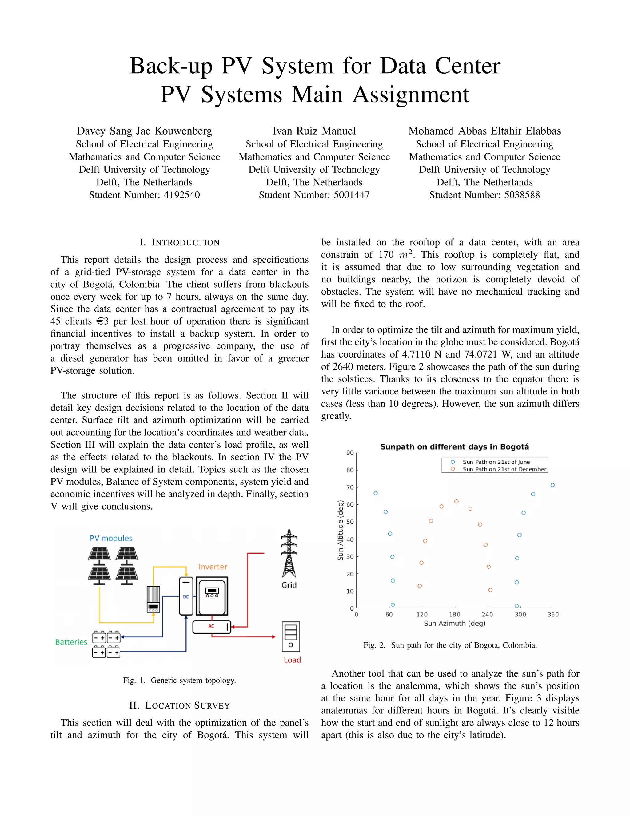
2. Fig. 3. Analemmas for different hours for the city of Bogota, showcasing
fairly stable 12 hours of sunlight throughout the year thanks to the city’s
latitude.
In order to correctly calculate the optimal panel tilt and
azimuth weather data has to be used. DNI, DHI and GHI
data for the whole year was obtained by using Meteonorm.
With it the Irradiance incident on the module can be obtained
following equation 1.
Gmod = Gdirect + Gdiffuse + Galbedo (1)
With Gdirect = DNI ∗ cos(AOI), where AOI is the
time-dependant angle of incidence (or Plane of the Array).
Gdiffuse = SV F ∗DHI according to the Isotropic sky model
[2]. Other, more precise models are available, but the Isotropic
model’s simplicity suits our hypothetical case well enough.
Finally, Galbedo = GHI ∗ α ∗ (1 − SV F), where α is the
albedo of the surrounding area, and SVF is the Sky View
Factor, described in equation 2.
SV F =
1 + cos(θM )
2
(2)
By integrating the radiance incident on the module for all
possible surface tilts and azimuths an irradiation profile is
obtained.
Figure 4 shows the irradiation profile for the city of Bogot´a.
It states that the maximum irradiation is obtained with a
surface tilt of 9 degrees and surface azimuth of 128 degrees.
Fig. 4. Optimization of the panel tilt and azimuth for Bogot´a, giving optimal
panel tilt and azimuth of 9 and 128 degrees respectively.
III. LOAD ANALYSIS
The load profile for the data centre was created by manipu-
lating the provided data, including the daily percentile pattern
and the monthly electricity bill. These were combined to create
the hourly load profile for the whole year, peaking at 8.5 kW
during the day, while dropping to around 6 kW at night. A
sample of the first day of each month is shown in figure 5.
Note the near zero difference between months; while there
are differences between each month in terms of total energy
consumption, these variations are too small to show up in the
final load pattern.
Fig. 5. A sampling of the load profile for the first day of each month. The
load peaks consistently at around 8.5 kW during the day, while bottoming out
at just over 6 kW during the night. Note the nearly complete absence of any
variation between months.
As stated in the assignment, a blackout occurs every week,
at which point the data centre moves away from its normal
load profile and switches to its critical load. The PV portion
of the system will not work during blackouts, even if they
2

3. happen during the day. A simulink model of the system was
developed to simulate these situations.
A visual representation is shown in figure 6, with the
critical load shown in orange. While the blackout is supposed
to occur at random on the same day each week, for the
implementation in the model, 10 AM was chosen, as it
would take away the most time from the PV system
to recharge the battery/provide support for the nominal
load. This, coupled with a potential week with low solar
irradiance due to cloud coverage would constitute a worst
case scenario.
Fig. 6. One typical week of load for the datacentre. The blackout occurs at
10 AM on Sunday, as indicated in red, lasting for 7 hours. At this time, the
load decreases to maintain just a critical load of 5.8 kW.
A key requirement is that the output of the PV system
cannot exceed the data center’s load at any time. Figure 7
show’s the net difference between the PV system and the
required load for the whole year. It shows how the system
is not oversized and complies with the constrains stated by the
client.
Fig. 7. Load not supplied by the PV system throughout the whole year.
IV. PV DESIGN
In this section, the process of designing the back-up PV
system for a data center in Bogota, Colombia is described
separately for each system component.
A. PV modules/array
After considering the location properties and calculating the
optimal tilt angle and orientation in section II, the temperature
model of Sandia, described in [1], is used to calculate the
efficiency of the given two modules. The first module, the
Cheetah 72M 380-400 Watt, is found to give the best
performance. Even though the temperature coefficients are
almost the same for both modules, and the second module has
higher STC values, the second module (Cheetah 72M 390-410
Watt half-cell) has double the number of cells and thus, the
effect of any temperature increase is more severe and yields a
lower output. The area of the chosen module is 1.98 m2
.
Based on the load analysis discussed in section III
and after including all the efficiencies in the system (PV
module, charge controller and inverter), the maximum
number of modules is found to be 21, more than that
and the PV output would exceed the load. Considering
the charge controller limitations (discussed in subsection
IV-B1) 18 modules were chosen for a system of 3 charge
controllers.
This number of panels provides sufficient amount of energy
to fully charge the batteries before the blackout and able to
maximally support the grid (increase the saving) during normal
operation. Additionally, in this configuration there is a room to
expand the system by 6 extra modules with the same number
of inverters, if the constrains of the system change and some
cabling changes are permitted.
Since the location is a valley with a horizon free of
obstacles, the row to row shading is considered for a roof area
of 170 m2
. Due to the fact that the cable connection cost
is very low, the shading free time window taken during
winter solstice (the 21st of December) is from 7 am to
5 pm. For this period, the module spacing is found to
be 3.2516 m and the total area is 58.6462 m2
for 3 by 6
arrangement. This gives a Ground Cover Ratio (GCR) of
0.6086 (total area/PV area).
B. BoS components
1) Charge Controllers (MPPT): Two charge controllers
were given as options for the system: the Conext MPPT 60-
150 and the Conext MPPT 80-600. Table IV-B1 displays the
most important parameters for each model.
TABLE I
CHARGE CONTROLLER PARAMETERS
Model Pmax IarrSC VstrOC Io max η48V Cost
60-150 3500W 48 A 150 V 60A 98% 530e
80-600 4800W 28 A 550 V 80A 96% 1200e
For this system the Conext MPPT 60-150 will be used,
primarily due to its low cost. Our 18 PV panel configuration
3

4. would require either three Conext MPPT 60-150 or two Conext
MPPT 80 600.
Since two of the former can be bought for less than one
of the latter, and since charge controllers are a relatively
expensive component, it makes economical sense to use them.
Several design limitations constrain the configuration for the
Conext MPPT 60-150 charge controller. First, Pmax limits the
total number of panels to 8 (3500), as shown in 3.
NT max =
Pmax
PMP P
=
3500W
400W
= 8 (3)
However, the maximum number of panels is also determined
by the DC output voltage, which has been set to 48 V on our
system due to our battery configuration and inverter voltage
requirements. Equation 4 establishes that no more then 7
panels can be connected to the charge controller.
N48V max =
VOCST C · Io max
PMP P
=
48V · 60A
400W
= 7 (4)
The maximum number of panels in series can be deduced
by using VstrOC as the upper limit. Since VOCST C = 49.8V ,
this limits the number of panels per string to 3, as shown in
equation 5.
Nstring max =
VstrOC
VOCST C
=
150V
49.8V
= 3 (5)
In order to maintain a constant voltage per string, and
reduce current losses in the system, a configuration of six
panels per charge controller will be used. The panels will be
connected in arrays of two strings of three panels each. A
total of three 60-150 MPPT charge controllers will be used.
2) Inverter: Two different inverters were available for this
project: the Context XW Pro for EMEA/APAC and the Context
XW Pro for North America. They are essentially the same
model, with some small key differences in terms of voltage
and frequency operation. Both are capable of single and three
phase operation.
According to our assignment specifications, the data
center in Bogot´a operates at a Voltage of 240 V and a
frequency of 60 Hz. This narrows down the inverter to
the second, the North American model which is compatible
with those requirements.
Table IV-B2 displays key inverter specifications.
TABLE II
INVERTER SPECIFICATIONS
Pinv maxDC IinDCmax Vin Ioutmax VoutAC ηCEC
8500 W 180 A 48 V 52 A 240 V 93%
Inverter selection depends primarily on the maximum STC
power output, defined in equation 6. Our panels are have a
maximum power output of 400W, and we are using 18 of
them. Thus, PST C
DC = 7200W.
PST C
DC = NT · PST C
MP P (6)
Equation 7 establishes the selection rule for the inverter.
Since Pinv maxDC = 7200W, our system of 18 panels is
well within operating limits.
Pinv maxDC > PST C
DC (7)
The maximum DC STC power approximately the same as
the nominal DC power of the plant (PST C
DC ≈ PDC0). Since we
have configured our batteries and charge controllers to work
at 48 V, our maximum DC current cannot exceed 150 A. This
is also within operating limits.
Finally, the inverter is responsible for charging and discharg-
ing the batteries. More details about the battery configuration
are given in section IV-B3.
Based on the inverter parameters and the variable
DC input power during the day, the Sandia National
Laboratories (SNL) model for the inverter efficiency is
used to plot the hourly inverter efficiency during the first
day of each month for one year operation period. The
figure is attached in the appendix VI.
3) Battery: The number of batteries in a system can be
calculated by the following equation:
Nbatt =
SF · Eout
DoD · η · Cbatt
(8)
where SF is the sizing factor, Eout is the total required energy
the battery system is supposed to provide, η is the battery
discharge efficiency DoD is the depth of discharge, Cbatt is
the battery energy capacity.
The batteries at our disposal is rated at 12 V and between
190 and 210 Ah depending on the rate of discharge. Due to
the rate of discharge, it is safe to assume the lower limit will
apply to this case, giving a total energy capacity of 2.28 kWh
per battery. The Depth of Discharge will be limited to 0.6
to protect the batteries and increase their lifespan. The
critical load draws 5.8 kW for 7 hours. The sizing factor SF
is set at 1.1 to ensure that the batteries cannot be discharged
past their safe DoD limits. The discharge efficiency is equal
to the SNL inverter efficiency model (90.98%). Combining
these factors, the total number of batteries becomes:
1.1 · 40.6 kWh
0.6 · 90.98% · 2.28 kWh
= 36 (9)
Since the batteries are to be connected to the inverter,
they can be arranged as 12 strings, where a string consists
of 3 batteries in series to give 48 V. This remains within the
inverter’s maximum battery Ah limit (10000Ah).
4) Cables: For connecting the PV panels with the charge
controller, the short circuit of the panel is taken for the
cable sizing. Since there are two parallel strings per charge
controller, the short circuit current flowing in the cable is
ISC = 2 · 10.36 = 20.72 A. For simplicity, the cables are
4

5. assumed to have no sun exposure and thus no temperature cor-
rection factor. Therefore, Ampacity = 1.56·20.72 = 41.44 A.
This gives a Wire Cross-Section Area of 10 mm2
which equals
a Wire Size of 8 AWG based on UL 486E and IEC 60998-1.
For the DC bus connecting the batteries with the inverter,
two ways to find the maximum DC current input to the inverter
are considered:
• While connected to the grid and assuming the battery is
fully charged, the maximum current is the aggregation
of the short circuit currents from the charge controllers.
Thus, ISC = 3 · 20.72 = 62.16 A and Ampacity =
1.56 · 62.16 = 96.97 A.
• During blackout, the maximum current drawn from the
battery is calculated using the power required to sup-
ply the critical load (assuming the battery bank can
instantaneously supply it) Imax = PDC/V48. Using
the inverter efficiency and Pcritical
AC = 5.8 kW PDC
is found to be 6.375 kW. Thus, Imax = 132.8A and
Ampacity = 1.56 · 132.8 = 207.2.
In this system layout, the charge controller is only respon-
sible of providing Maximum Power Point Tracking (MPPT)
functionality. Hence, during the blackout the charge controller
is not operating and the only component that limits the
maximum current that the system can provide is the
inverter. The maximum current present on the system dur-
ing the blackout can be found by dividing the maximum
powers at the inverter terminals by their respective voltages.
Based on the simulation result, these values are found to be
PDCmax = 6.955 kW and PACmax = 6.284 kW. the max-
imum currents during the blackout are IDC
max = 144.90 A
and IAC
max = 2.62 A.
C. DC and AC yield
The instantaneous DC side yield is defined by equation 10.
DCY (t) =
PAC(t)
PST C
(10)
The instantaneous DC side yield of the proposed system is
shown in figure 8. Not that during a short period of time the
yield exceeds 100%. This is due to an hour with extremely
high solar irradiance, exceeding STC values.
Fig. 8. The instantaneous DC side yield. Due to high irradiance hours, the
maximum side yield occasionally exceeds 100%.
Similarly, the instantaneous AC side yield is defined in
equation 11.
ACY (t) =
PAC(t)
PST C
DC
(11)
The AC side yields takes into account power losses in the
wires, charge controller, inverter, and other components,
while the DC side yield does not. This is reflected in figure
9; the shape of the graph is nearly exactly the same as figure
8 but shifted downwards.
Fig. 9. The instantaneous AC yield of the PV system.
D. System losses
Due to the several efficiency elements, a certain amount of
power from the PV panels is expected to be lost. The system
losses are shown in figure 10. The low level losses are due to
losses in the charge controller, the lines connecting the charge
controller and the inverter, and the inverter itself. The large
peaks are due to the outage hours, during which the generated
power cannot be used by the load or to charge the battery.
5

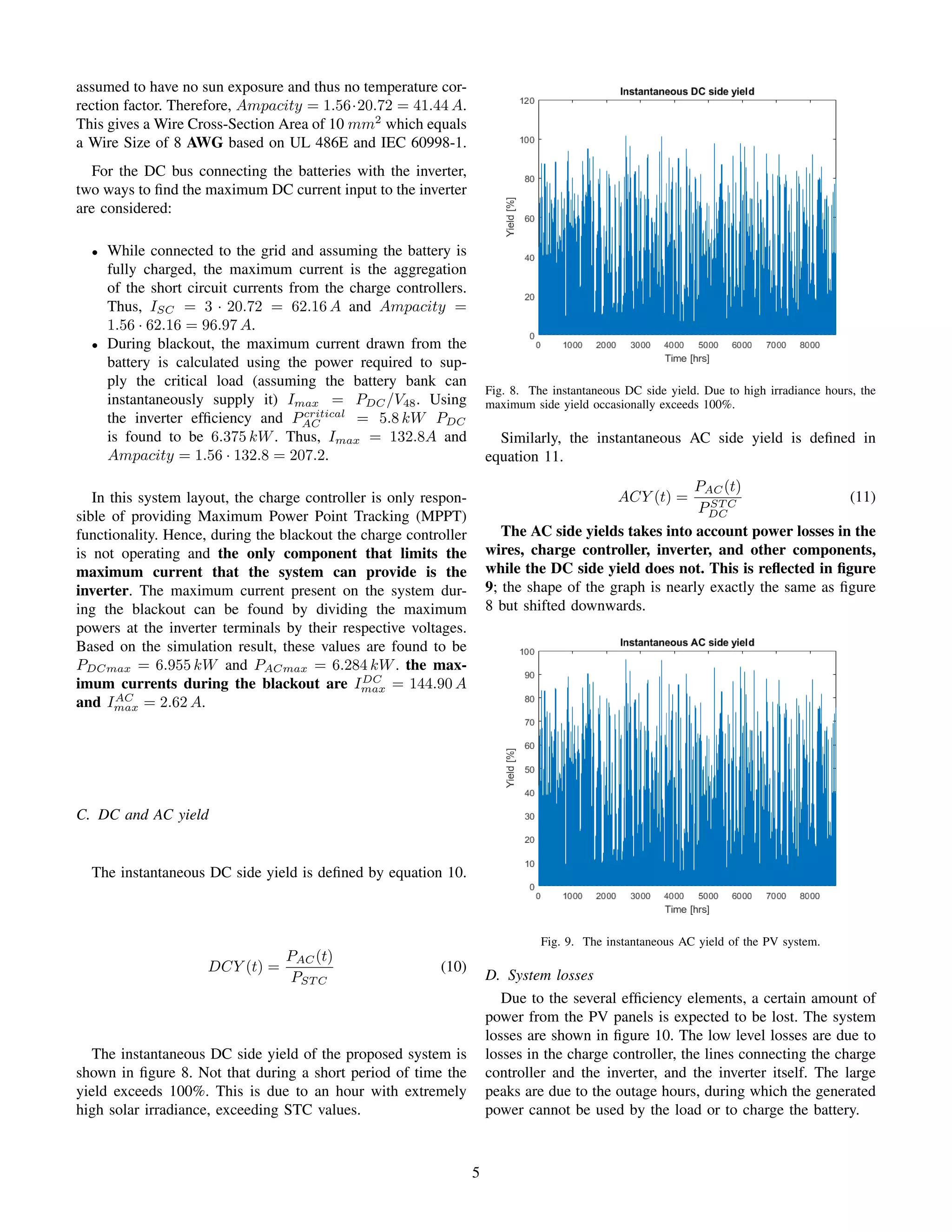
6. Fig. 10.
Dividing the total losses by the raw output of the PV panels,
the total fraction of energy lost lies at around 10%. Most of
these losses are incurred in the inverter and during the outage
hours.
E. Cost analysis
Table IV-E lists the given prices for all the system compo-
nents, either by installed Wp or number of units. Using the
values provided, the overall cost of the system is e33,298.
This accounts for 18 PV panels (7200 Wp), 36 batteries, 3
charge controllers (type 1) and 1 inverter, plus switchgear
(assumed to be 1 of each).
TABLE III
ASSOCIATED COST FOR EQUIPMENT
Equipment Cost e/Wp Cost e/Unit
Solar panels 0.87 -
Hybrid Inverter 0.64
Mounting Structure - 32
Charge Controller 1 - 530
Charge Controller 2 - 1200
Battery - 430
DC/DC Switchgear - 370
AC/AC Switchgear - 450
Accessories 0.55 -
Table IV-E lists the cost of electricity and outage compensa-
tion per client for the data center. According to our model, our
system generates a total of 5598.1 kWh of electricity saved
per year, or an equivalent of e1119.62 saved per year.
Assuming 100% component reliability, and that the blackouts
occur at the same day of the week for up to 7 hours, the system
is guaranteed be able to supply the critical load throughout the
year. This means that the client avoids having to pay up to
e49140 in compensation costs.
This bring total savings to e50259.62 per year of operation.
TABLE IV
ASSOCIATED COSTS FOR ELECTRICITY AND OUTAGE COMPENSATIONS.
Location N. clients Compensation e/h Elec. price e/kWh
Bogot´a, CO 45 3.00 0.20
In terms of savings, the prevention of not providing the
critical load is the most significant. This saving alone easily
justifies the e33,298 investment for the PV storage system.
Furthermore, the PV system cuts down on the electricity bill by
supplying energy to the load. The long lifetime of the system
justifies the sizing.
According to our simulations, there are economies of scale
in relation to the system’s size (limited by the constrain of not
exceeding the building’s load). Table IV-E compares electricity
saving returns vs system cost for various configurations. Since
a bigger system also provides more critical load security, the
advantages of our configuration are apparent.
TABLE V
ELECTRICITY SAVINGS VS SYSTEM COST FOR VARIOUS CONFIGURATIONS
N. panels N. CC Elec. savings (10yr) Cost Relation
8 1 e2542.2 e23678 10.7%
16 2 e9476.8 e31056 30.5%
18 3 e11196.2 e33298 33.6%
V. CONCLUSION
In this report, the process of designing a back-up PV system
for a data center located in Bogota, Colombia was discussed
based on the provided constraints and components options.
To fully supply the critical load of 5.8 kW, 18 PV panels
of type Cheetah 72M 380-400 Watt from the manufacturer
Solar Jinko with 36 batteries of type 8A4DLTP-DEKA from
the manufacturer MK Battery are found to be the optimal
choice to save the company from a weekly 7 hour blackout.
The system requires three charge controllers of type ConextTM
MPPT 60 150 from the manufacturer Schneider Electric and
an inverter of type ConextTM
XW Pro for North America from
the same manufacturer.
Thanks to the high irradiance in Bogota, the DC yield of
the system exceeds a 100% of the standard DC output power
during the summer period. Even after subtracting the lost PV
output power due to the regular blackout, the system is still
prolific enough to provide a total saving of e50259.62 per
year. Therefore, beside the environmental benefits, the system
has a strong business case by having an attractive Return On
Investment (ROI) of only 0.60 years.
REFERENCES
[1] Kanyawee Keeratimahat, A.G. Bruce, J.K. Copper, et al.
“Temperature estimation of an unconventional PV array
using the sandia module temperature model”. In: Bris-
bane: Asia Pacific Solar Research Conference. 2015.
[2] P.G. Loutzenhiser et al. “Empirical validation of models
to compute solar irradiance on inclined surfaces for build-
ing energy simulation”. In: Solar Energy 81.2 (2007),
pp. 254–267.
6

7. VI. APPENDIX
Fig. 11. The inverter efficiency for the first full day of solar output to the
load for each month.
7