This document provides a lecture plan for teaching Unit 1 of the Design and Analysis of Algorithms course. The unit covers introduction topics including the notion of algorithms, algorithmic problem solving, analysis of algorithm efficiency, and asymptotic notations. The lecture plan lists 9 topics to be taught over 9 class periods using modes of delivery like PPT and blended learning. It also includes examples of activity based learning like flashcards, programming skills tests, and a crossword puzzle to reinforce the topics.


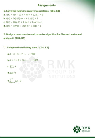
![Unit I INTRODUCTION
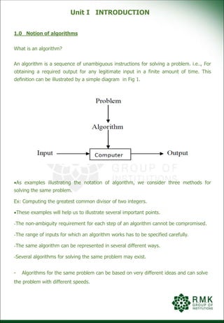
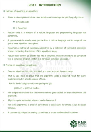
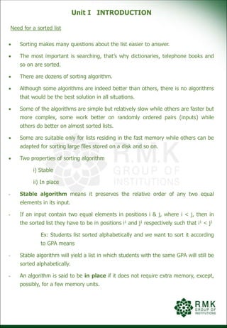
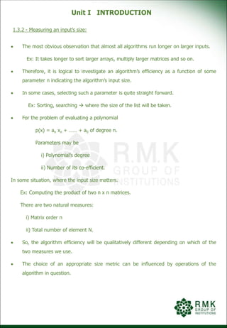
Algorithm: Sieve(n)
for p 2 to n do A[p] p
for p 2 to [ 𝑛] do
if A[p] ≠ 0
j p*p
while j < n do
A[j] 0
j j+p
i 0
for p 2 to n do
if A[p] ≠ 0
L[i] A[p]
i i+1
return L
So, we incorporate the sieve into middle school procedure to get a legitimate algorithm for
computing gcd.
1.1 Fundamentals of algorithm problem solving
Sequence of steps in designing & analyzing an algorithm.
Understanding the problem:
Before designing an algorithm is to understand completely the problem.
Read the problems description and ask questions or doubt about the problems.
Solve the few small examples by hand.
Think about special cases and ask questions again if needed.
There are few types of problems that arise in computing applications quite often.
There are known algorithms for solving it. It might help us to understand how such an
algorithm works and know its strengths and weakness.](https://image.slidesharecdn.com/cs8451daaunit-i-220422035930/85/CS8451-DAA-Unit-I-pptx-29-320.jpg)
![Unit I INTRODUCTION
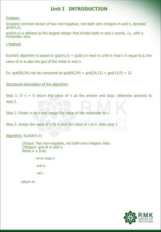
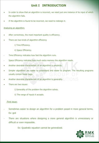
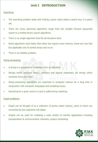
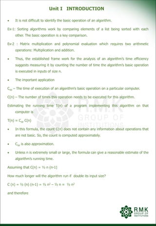
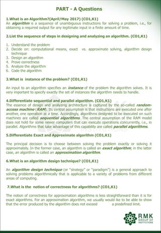
Ex: Measuring input’s size for spell checking algorithm.
i) If the algorithm examines individual characters of its input, then measure the
size by the number of characters.
ii) If it works by processing words, should count their number in the input.
Should make a special note about measuring size of inputs for algorithms involving
properties of numbers.
Ex: Checking for prime.
Computer scientists prefer measuring size by the number of bits b in the n’s binary
representation.
b = [log2 n]+1
This gives the efficiency of algorithms.
1.3.3 - Units for measuring running time:
Concerns about units of measuring an algorithm’s running time.
We can simply use some standard unit of time measurement – a second, a millisecond
and so on to measure the running time of a program implementing the algorithm.
Drawbacks:
i) Dependence on the speed of a particular computer.
ii) Dependence on the quality of a program implementing the algorithm.
iii) The compiler used in generating the machine code.
iv) The difficulty of clocking the actual running time of the program.
We should have a metric that does not depend on these extraneous factors.
One possible approach is to identify the most important operation of the algorithm,
called the basic operation. The operation contributing the most for the total running
time and compute the number of times the basic operation is executed.](https://image.slidesharecdn.com/cs8451daaunit-i-220422035930/85/CS8451-DAA-Unit-I-pptx-42-320.jpg)
![Unit I INTRODUCTION
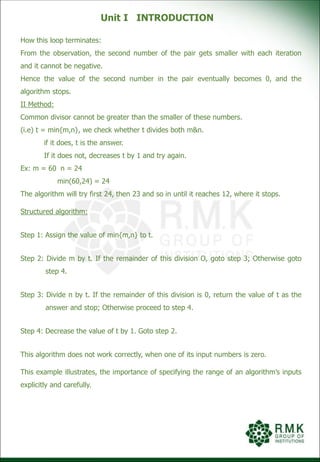
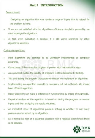
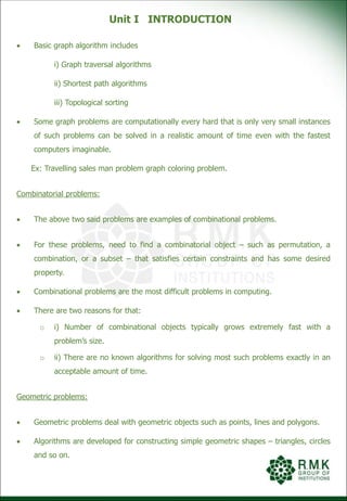
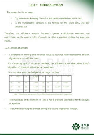
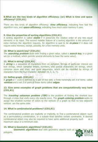
On the other hand of the spectrum are the exponential function 2n and n!. Both these
functions grow so fast that their values become astronomically large even for rather
small values of n.
Another way to appreciate the qualitative difference among the orders of growth of
the functions in table is if we increase two fold in the value of their argument n.
The function
log2 n => log2 2n = log2 2 + log2 n = 1+log2 n => increases in value by just 1.
n log2 n => 2n log2 2n = 2n [1+log2 n] => increases slightly more than 2 fold.
n2 => (2n)2 = 4n2 => 4 fold
n3 => (2n)3 = 8n3 => 8 fold
n! = increases much more than the above
1.3.5 - Worst-case, Best-case and Average-case Efficiencies:
To measure an algorithm’s efficiency as a function of a parameter indicating the size of
the algorithm’s input.
But there are many algorithms for which running time depends not only on an input
size but also on the specific of a particular input.
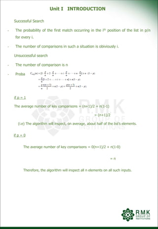
Ex: Sequential search.
This is a straight forward algorithm that searches for a given item in a list of n
elements by checking successive elements of the list until either a match with the
search key is found or the list is exhausted.](https://image.slidesharecdn.com/cs8451daaunit-i-220422035930/85/CS8451-DAA-Unit-I-pptx-45-320.jpg)
![Unit I INTRODUCTION
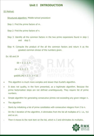
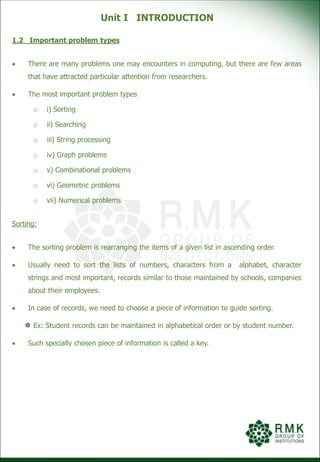
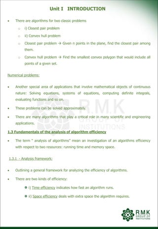
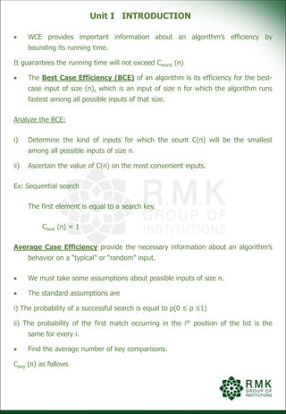
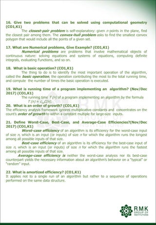
Algorithm:
Sequential search (A[0… n-1], K)
// Input: An array A[0…n-1] and a search key K.
// Output: Returns the index of the first element of A that matches K or -1 if there are no
matching elements.
i 0
while i < n and A[i] ≠ K do
i i+ 1
if i < n return i
else return -1
The running time of this algorithm can be quite different for the same list size n depends
where the K appears.
In the worst case, when there are no matching elements or the first matching element
happens to be the last one on the list, the algorithm makes the largest number of key
comparisons among all possible inputs of size n:
Cworst (n) = n
The Worst Case Efficiency (WCE) of an algorithm is its efficiency for the worst-case
input of size n, which is an input of size n for which the algorithm runs the longest among
all possible inputs of that size.
Computing worst-case efficiency is straight forward, analyze what kind of inputs yield the
largest value of the basic operation’s count C(n) among all possible inputs of size n and
then compute the worst-case value
Cworst (n)](https://image.slidesharecdn.com/cs8451daaunit-i-220422035930/85/CS8451-DAA-Unit-I-pptx-46-320.jpg)
![Unit I INTRODUCTION
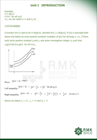
1.4.6 Properties of Asymptotic Notations
Theorem: If t1(n) ε O(g1(n)) and t2 ε O(g2(n)) then t1(n)+t2(n) ε
O(max{g1(n),g2(n)})
Proof: simple fact about four arbitrary real numbers a1, a2, b1, b2: if a1 ≤ b1 and a2 ≤
b2, then a1+a2 ≤ 2 max{b1,b2}.
Since if t1(n) ε O(g1(n)), there exist some positive constant c1 and some nonnegative
integer n1 such that
t1(n) ≤ c1g1(n) for all n≥n1
Since if t2(n) ε O(g2(n)), t2(n) ≤ c2g2(n) for all n≥n2
Let us denote c3=max{c1,c2} and consider n≥max{n1,n2} we can use both inequalities.
T1(n)+t2(n)≤c1g1(n)+c2g2(n)
≤c3g1(n)+c3g2(n)=c3[g1(n)+g2(n)]
≤c32max{g1(n),g2(n)}
So t1(n)+t2(n) ε O(max{g1(n),g2(n)})
It implies that the algorithm’s overall efficiency is determined by the part with a larger
order of growth.
1.4.7 Comparing Order’s of Growth using Limits.
Though definitions of Ο, Ω and θ are indispensable for proving their abstract properties,
they are rarely used for comparisons of orders of growth of two specific functions.
A much more convenient method for doing so is based on computing the limit of the
ratio of two functions.
Three principal cases may arise
0 implies that t(n) has a smaller order of growth than g(n)
c > 0 implies that t(n) has a same order of growth as g(n)
∞ implies that t(n) has a larger order of growth than g(n)
First two cases mean that t(n) Ο(g(n))
Last two cases mean that t(n) Ω(g(n))
Second case mean that t(n) θ(g(n))
=](https://image.slidesharecdn.com/cs8451daaunit-i-220422035930/85/CS8451-DAA-Unit-I-pptx-53-320.jpg)
![Unit I INTRODUCTION
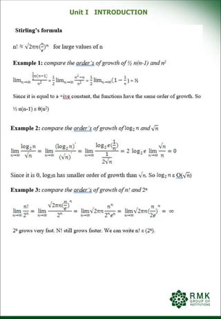
Problem: Finding the value of the largest element in a list of n numbers.
Assumption: List is implemented as array.
Algorithm:
maxval A[0]
for i 1 to n-1 do
if A[i] >maxval
maxval A[i]
return maxval
Applying general framework outlined.
i) Measuring an input’s size:
- The input size is the number of elements in the array i.e.., n
i) Units for measuring running time:
- The operations most often executed are in the for loop.
- There are two operations
o Comparison A[i] >maxval
o Assignment maxval A[i]
Which have to consider?
- Comparison is executed on each repetition of the loop
- Assignment is no. So, the basic operation is comparison
The number of comparisons will be the same for all arrays of size n. There is no need
to distinguish among the worst, average and best cases.
Count the number of times the basic operation performed and try to formulate as
function of size n.
The algorithm makes one comparison on each execution of the loop, which is
repeated for each value of the loop’s variable I within the bounds between 1 and n-1.
𝐶 𝑛 =
𝑖=1
𝑛−1
1 =>
𝑖=1
𝑛−1
= 𝑛 − 1 − 1 + 1 = 𝑛 − 1 𝜖 𝜃(𝑛)](https://image.slidesharecdn.com/cs8451daaunit-i-220422035930/85/CS8451-DAA-Unit-I-pptx-57-320.jpg)
![Unit I INTRODUCTION
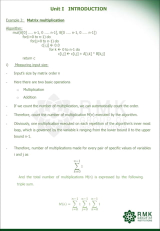
General plan for analyzing efficiency of non-recursive algorithms:
i) Decide on a parameter indicating an input’s size.
ii) Identify the algorithm’s basic operation.
iii) Check whether the number of times the basic operation is executed depends only on
the size of an input.
iv) Set up a sum expressing the number of times the algorithm’s basic operation is
executed.
v) Establish its order of growth.
Example 2: Element uniqueness problem
Algorithm:
for i 0 to n-2 do
for j i+1 to n-1 do
if A[i] = A[j] return false
return true
i) Measuring input’s size:
- The number of elements in the array- n elements
i) Measuring running time:
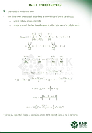
- The innermost loops contains a single operation.
- This is the basic operation
- The number of elements comparison will depend not only on n but also on whether
there are equal elements in the array and if there are, which array positions they
occupy..](https://image.slidesharecdn.com/cs8451daaunit-i-220422035930/85/CS8451-DAA-Unit-I-pptx-58-320.jpg)
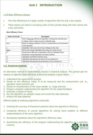
![Unit I INTRODUCTION
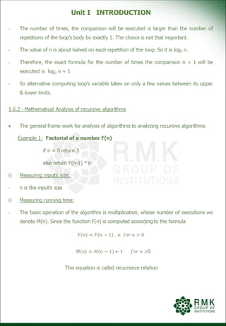
- To determine a solution uniquely for recurrence relation, we need an initial condition
that tells us the value with which the sequence starts.
- We can obtain this value by inspecting the condition that makes the algorithm stop its
recursive calls.
if n = 0 return 1
M(0) = 0
The call stop when n = 0
- Thus, we succeed in setting up the recurrence relation and initial condition for the
algorithm’s number of multiplication M(n):
M(n) = M(n-1) + 1 for n > 0
M(0) = 0
- There are two recursively defined functions
o Factorial function F(n)
o Number of multiplications M(n)
- For solving recurrence relations, we use the method of backward substitutions
M(n) = M(n-1) + 1 substitute M(n-1) = M(n-2) + 1
=[M(n-2) + 1] + 1 = M(n-2) + 2 substitute M(n-2) = M(n-3) + 1
= [M(n-3) + 1] + 2 = M(n-3) + 3
Therefore, general formula = M(n) = M(n-i) + i
M(n) = M(n-1) + 1 . . . . = M(n-i) + i = . . . . .
Initial condition n=0 so substitute i=n
M(n-n) + n = n](https://image.slidesharecdn.com/cs8451daaunit-i-220422035930/85/CS8451-DAA-Unit-I-pptx-63-320.jpg)
![Unit I INTRODUCTION
Solving recurrence relation equation by backward substitutions
M(n) = 2M(n-1) + 1 sub M(n-1) = 2M(n-2) + 1
= 2 [2M(n-2) + 1) + 1
= 22 M(n-2) + 2 + 1 sub M(n-2) = 2M(n-3) + 1
= 22 [2M (n-3) + 1] + 2 + 1
= 23 M(n-3) + 22 + 2 + 1
Therefore, after I substitutions, we get
M(n) = 2i M(n-i) + 2i-1 + 2i-2 + ……. + 2 + 1
= 2i M(n-i) + 2i -1
M(n) = 2n-1 M(n-(n-1)) + 2n-1 -1 n-i= 1, i= n-1
= 2n-1 M(n-n+1) + 2n-1 -1
= 2n-1 M(1) + 2n-1 -1
= 2n-1 + 2n-1 -1
= 2 . 2n-1 -1 = 2n -1
Thus we have an exponential algorithm, which will run for an unimaginably long time even
for moderate values of n. This is not due to the fact that this algorithm is poor.
It is the problem’s intrinsic difficulty that makes it so computationally difficult.
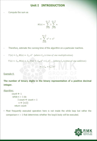
Example 3: Counting the number of binary digits
Algorithm: Bin Rec(n)
if n = 1 return 1
else return Bin Rec([n/2]) + 1](https://image.slidesharecdn.com/cs8451daaunit-i-220422035930/85/CS8451-DAA-Unit-I-pptx-65-320.jpg)
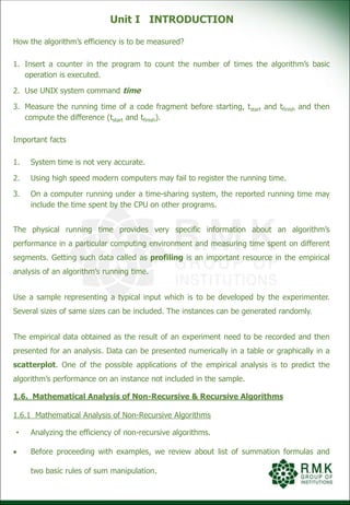
![Unit I INTRODUCTION
- The number of additions made in computing Bin Rec([n/2]) is A([n/2]), plus one more
addition is made by the algorithm to increase the returned value by 1.
A[n] = A([n/2]) + 1 for n > 1
- if n = 1, the recursive calls end, there are no additions made, the initial condition is
A(1) = 0
- The presence of [n/2] in the function’s argument makes the method of backward
substitutions stumble on values of n that are not powers of 2.
- Therefore the standard approach to solving such a recurrence is to solve it only for n
= 2k and then
o Apply the theorem called the smoothness rule.
o This theorem gives correct answer about the order of growth for all values of n.
- For n = 2k takes the form
A(2k) = A(2k-1) + 1 for k > 0
A(20) = 0
Now backward substitutions encounter no problems:
A(2k) = A(2k-1) + 1 substitute A(2k-1) = A(2k-2)+1
= [A(2k-2) + 1] + 1
= A(2k-2) + 2 substitute A(2k-2) = A(2k-3) + 1
=[A(2k-3) + 1] + 2
= A[2k-3] + 3
= A[2k-i] + i
= A[2k-k] + k](https://image.slidesharecdn.com/cs8451daaunit-i-220422035930/85/CS8451-DAA-Unit-I-pptx-66-320.jpg)


![Unit I Content Beyond Syllabus
Important Data Structures
Graphs:
A graph G=(V,E) is defined by a pair of two sets: A finite set V of items called vertices and
a set E of items called edges. If a pair of vertices (u,v) is same as (v,u) in a graph then the
graph is called as undirected graph. If pair of vertices (u,v) and (v,u) is not same in a graph
then it is called as directed graph or digraph. A graph with every pair of vertices connected
by an edge is called complete. A graph with relatively few possible edges missing is called
dense; a graph with few edges relative to number of its vertices is called sparse.
Graph representations: Adjacency Matrix and Adjacency List.
Adjacency Matrix: A graph with n vertices is represented by nxn matrix. The entries of the
matrix are 0 and 1. The entry A[u,v]=0 indicates there is no edge from u to v and A[u,v]=1
if the edge from u to v is present.
Adjacency List: Collection of linked lists, one for each vertex that contains all the vertices
adjacent to the particular vertex.
Weighted graph is a graph with numbers assigned its edges. These numbers are called as
weights. If this graph is represented by adjacency matrix A[u,v]=weight of the edge [u,v]
and ∞ if there is no edge. Such a matrix is called as weight matrix or cost matrix.
A path from vertex u to vertex v is sequence of adjacent vertices starts with u and ends
with v. length of the path is total number of vertices in a vertex sequence defining the path
minus 1. A directed path is a sequence of vertices in which every consecutive pair of the
vertices is connected by a directed edge. A graph is said to be connected if for every pair of
its vertices u and v there is a path from u to v. a graph with no cycles is said to be acyclic.
Trees:
A tree is a connected acyclic graph.
|E|=|V|-1 no of edges is no of vertices -1
Rooted trees: for every two vertices in a tree there exists one simple path from one of
these vertices to the other. Select an arbitrary vertex in a free tree and it is root.
Ancestors: for any vertex v in a tree, all the vertices on the simple path from the root to
that vertex are called ancestors of v.
Parent & child: if (u,v) is the last edge of the simple path from the root to vertex v, u is
parent and v is child.
Siblings: vertices that have same parent](https://image.slidesharecdn.com/cs8451daaunit-i-220422035930/85/CS8451-DAA-Unit-I-pptx-86-320.jpg)