DERIVATIVES
ELECTRONIC VERSION OFLECTURE
Dr. Lê Xuân Đại
HoChiMinh City University of Technology
Faculty of Applied Science, Department of Applied Mathematics
Email: ytkadai@hcmut.edu.vn
HCMC — 2024.
Dr. Lê Xuân Đại (HCMUT-OISP) DERIVATIVES HCMC — 2024. 1 / 55
OUTLINE
1 DERIVATIVES
2 HIGHERDERIVATIVES
3 LINEAR APPROXIMATIONS AND DIFFERENTIALS
Dr. Lê Xuân Đại (HCMUT-OISP) DERIVATIVES HCMC — 2024. 2 / 55
5.
OUTLINE
1 DERIVATIVES
2 HIGHERDERIVATIVES
3 LINEAR APPROXIMATIONS AND DIFFERENTIALS
4 RATES OF CHANGE AND RELATED RATES
Dr. Lê Xuân Đại (HCMUT-OISP) DERIVATIVES HCMC — 2024. 2 / 55
6.
Derivatives Tangents
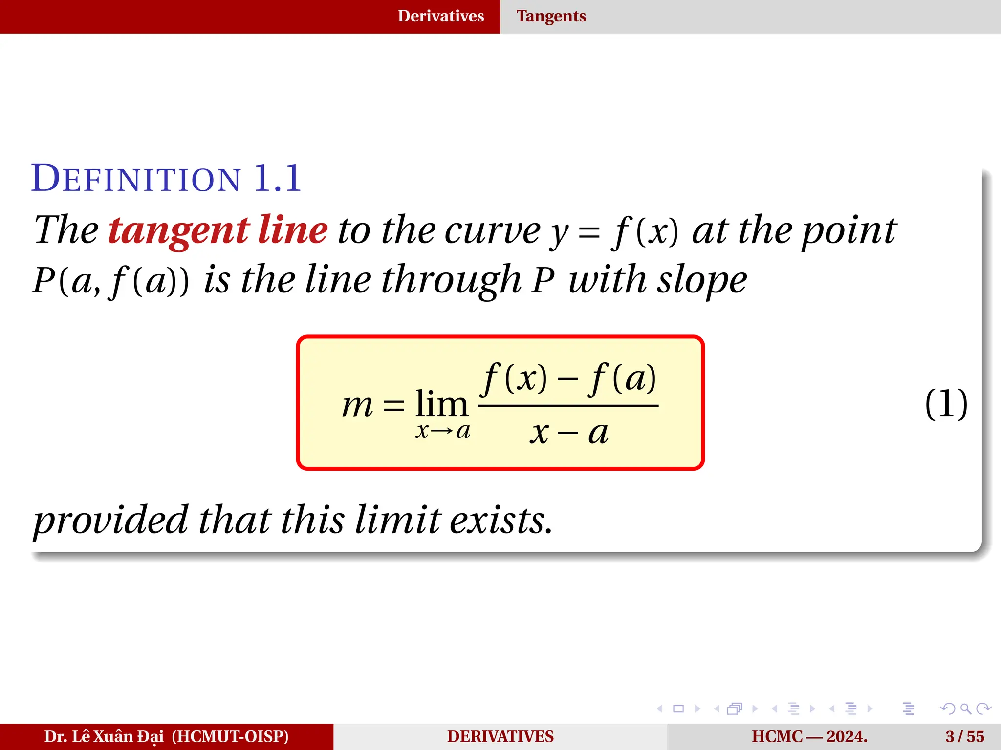
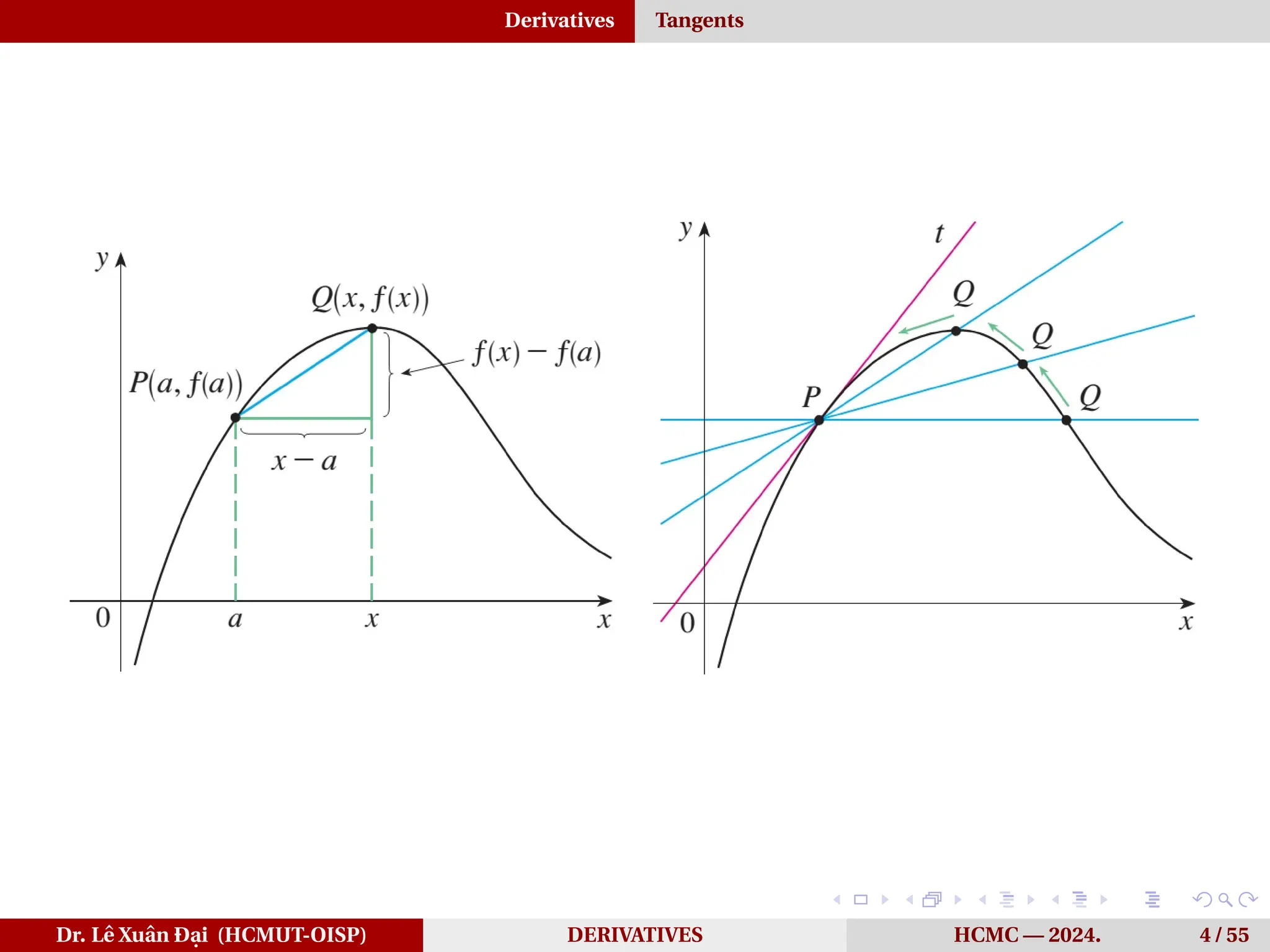
DEFINITION 1.1
Thetangent line to the curve y = f (x) at the point
P(a, f (a)) is the line through P with slope
m = lim
x→a
f (x)− f (a)
x − a
(1)
provided that this limit exists.
Dr. Lê Xuân Đại (HCMUT-OISP) DERIVATIVES HCMC — 2024. 3 / 55
Derivatives Tangents
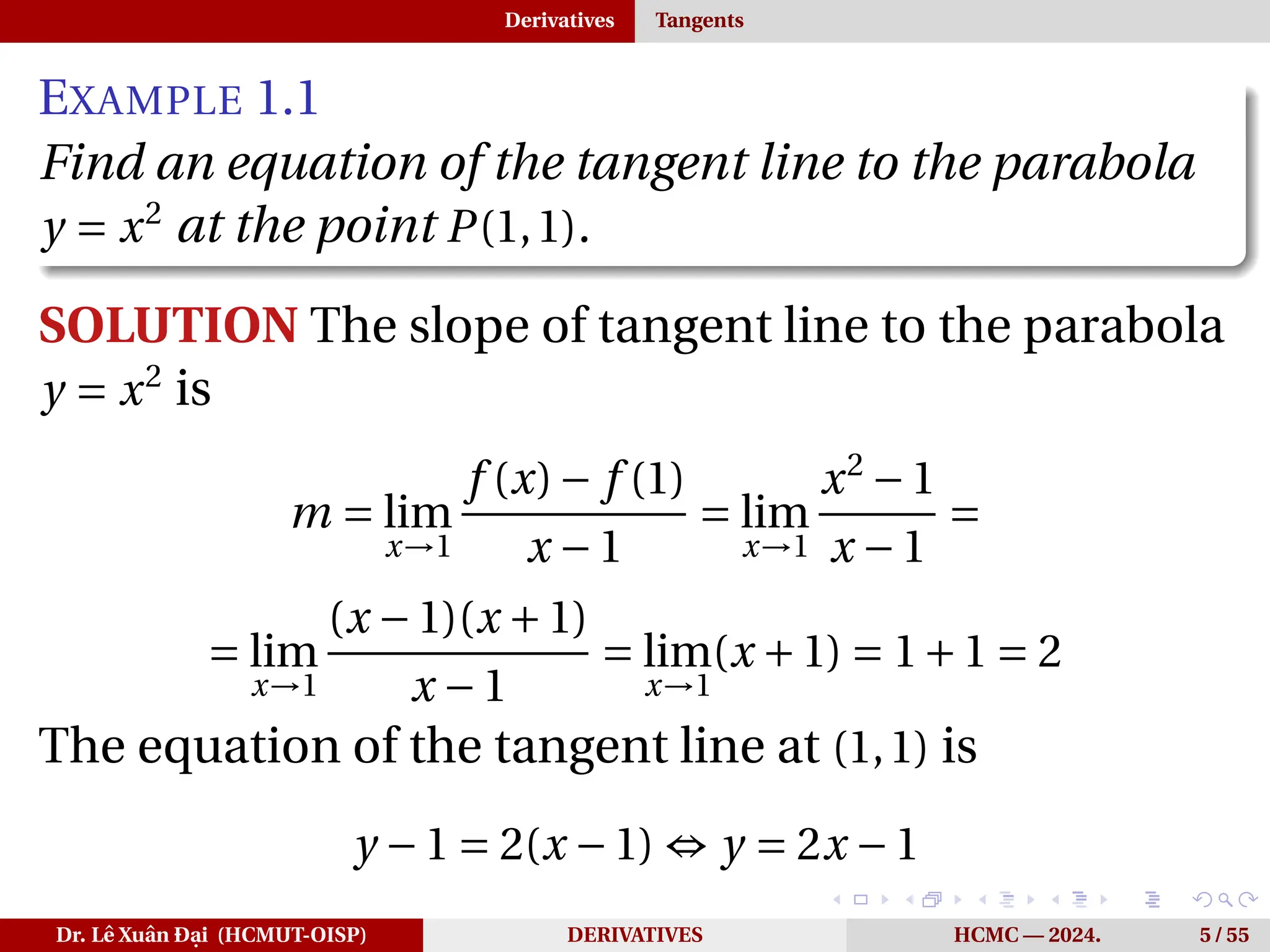
EXAMPLE 1.1
Findan equation of the tangent line to the parabola
y = x2
at the point P(1,1).
Dr. Lê Xuân Đại (HCMUT-OISP) DERIVATIVES HCMC — 2024. 5 / 55
9.
Derivatives Tangents
EXAMPLE 1.1
Findan equation of the tangent line to the parabola
y = x2
at the point P(1,1).
SOLUTION The slope of tangent line to the parabola
y = x2
is
m = lim
x→1
f (x)− f (1)
x −1
= lim
x→1
x2
−1
x −1
=
= lim
x→1
(x −1)(x +1)
x −1
= lim
x→1
(x +1) = 1+1 = 2
The equation of the tangent line at (1,1) is
y −1 = 2(x −1) ⇔ y = 2x −1
Dr. Lê Xuân Đại (HCMUT-OISP) DERIVATIVES HCMC — 2024. 5 / 55
10.
Derivatives Velocities
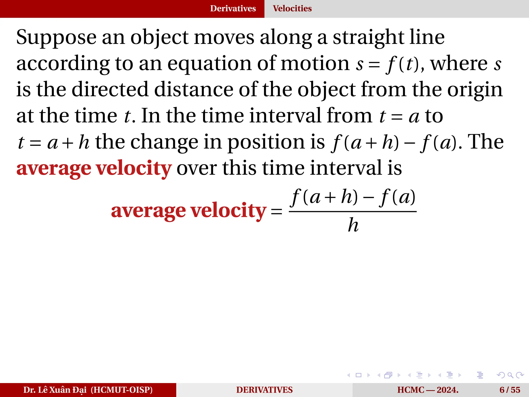
Suppose anobject moves along a straight line
according to an equation of motion s = f (t), where s
is the directed distance of the object from the origin
at the time t. In the time interval from t = a to
t = a +h the change in position is f (a +h)− f (a). The
average velocity over this time interval is
average velocity =
f (a +h)− f (a)
h
Dr. Lê Xuân Đại (HCMUT-OISP) DERIVATIVES HCMC — 2024. 6 / 55
11.
Derivatives Velocities
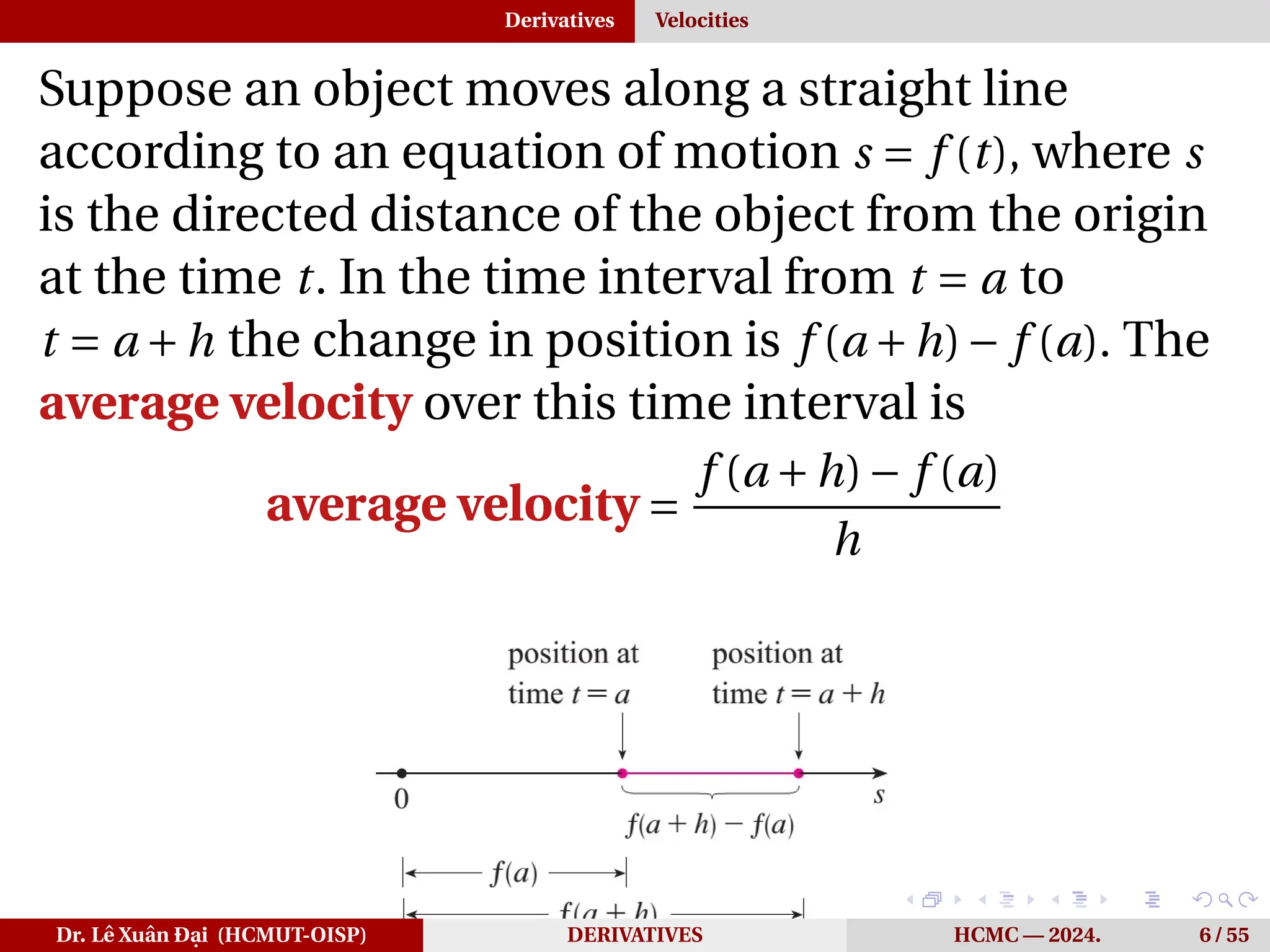
Suppose anobject moves along a straight line
according to an equation of motion s = f (t), where s
is the directed distance of the object from the origin
at the time t. In the time interval from t = a to
t = a +h the change in position is f (a +h)− f (a). The
average velocity over this time interval is
average velocity =
f (a +h)− f (a)
h
Dr. Lê Xuân Đại (HCMUT-OISP) DERIVATIVES HCMC — 2024. 6 / 55
12.
Derivatives Velocities
Now supposewe compute the average velocities
over shorter and shorter time intervals [a,a +h]. We
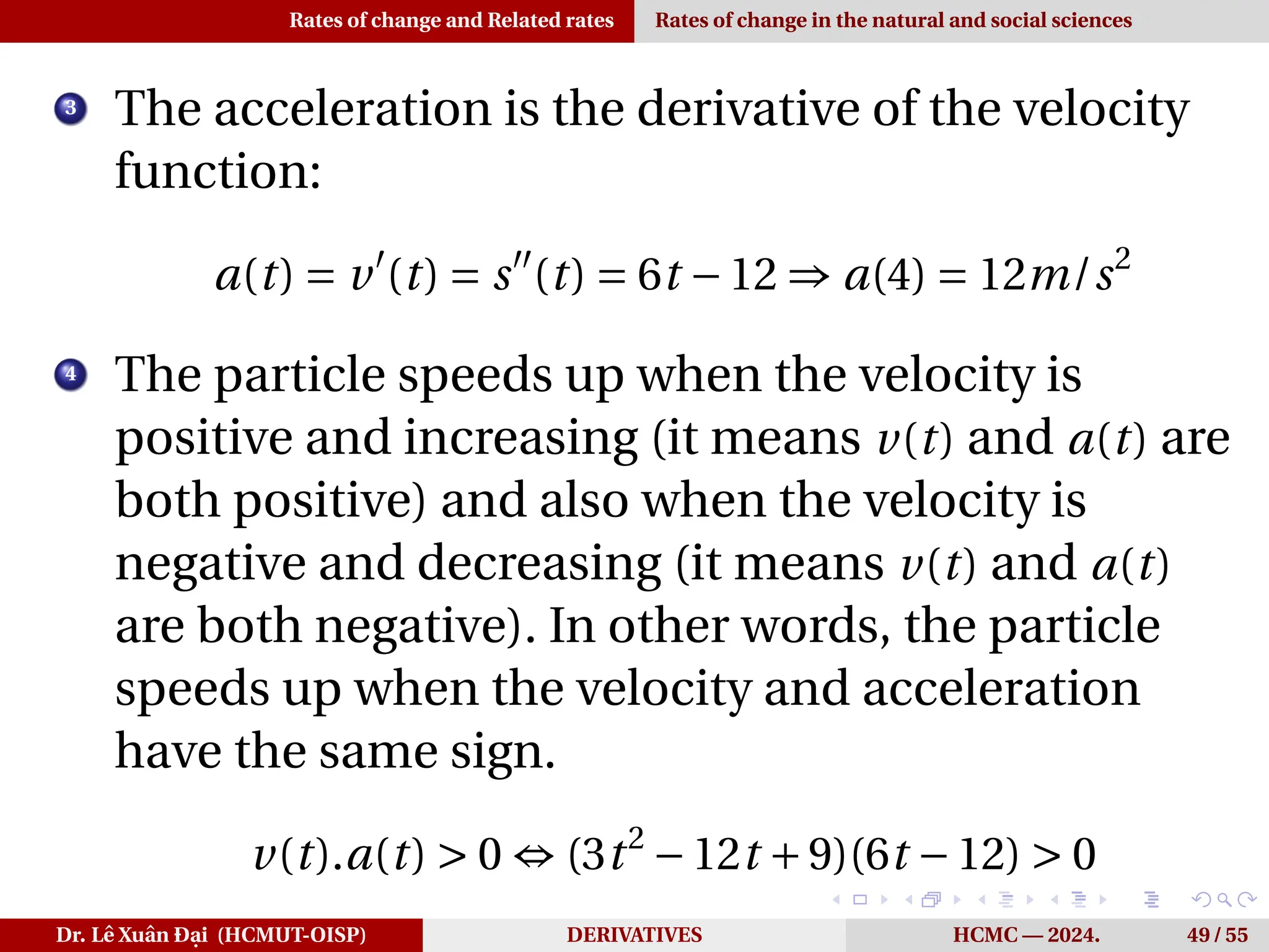
let h approach 0. The instantaneous velocity v(a) at
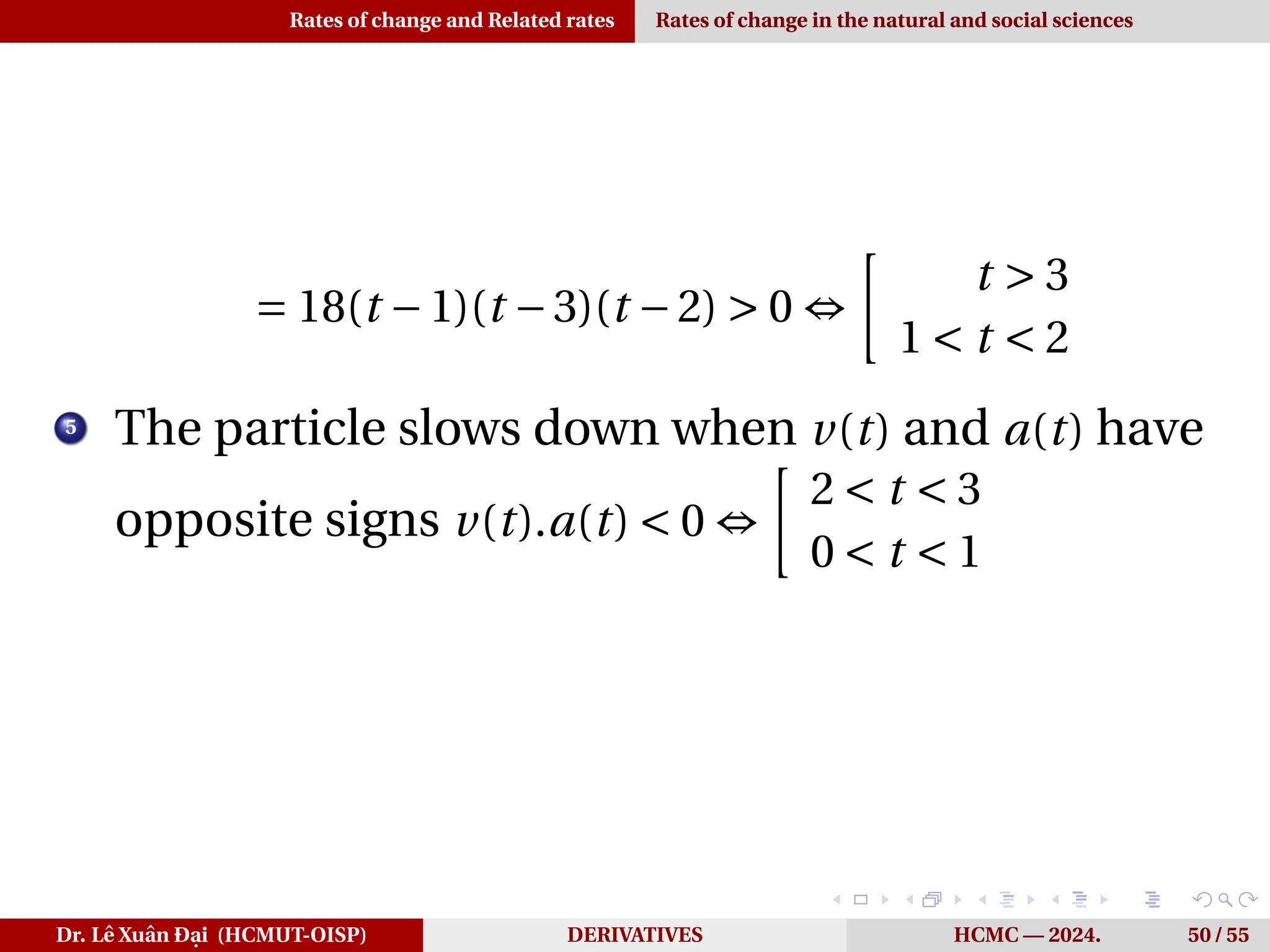
time t = a is defined by
v(a) = lim
h→0
f (a +h)− f (a)
h
(2)
Dr. Lê Xuân Đại (HCMUT-OISP) DERIVATIVES HCMC — 2024. 7 / 55
13.
Derivatives Velocities
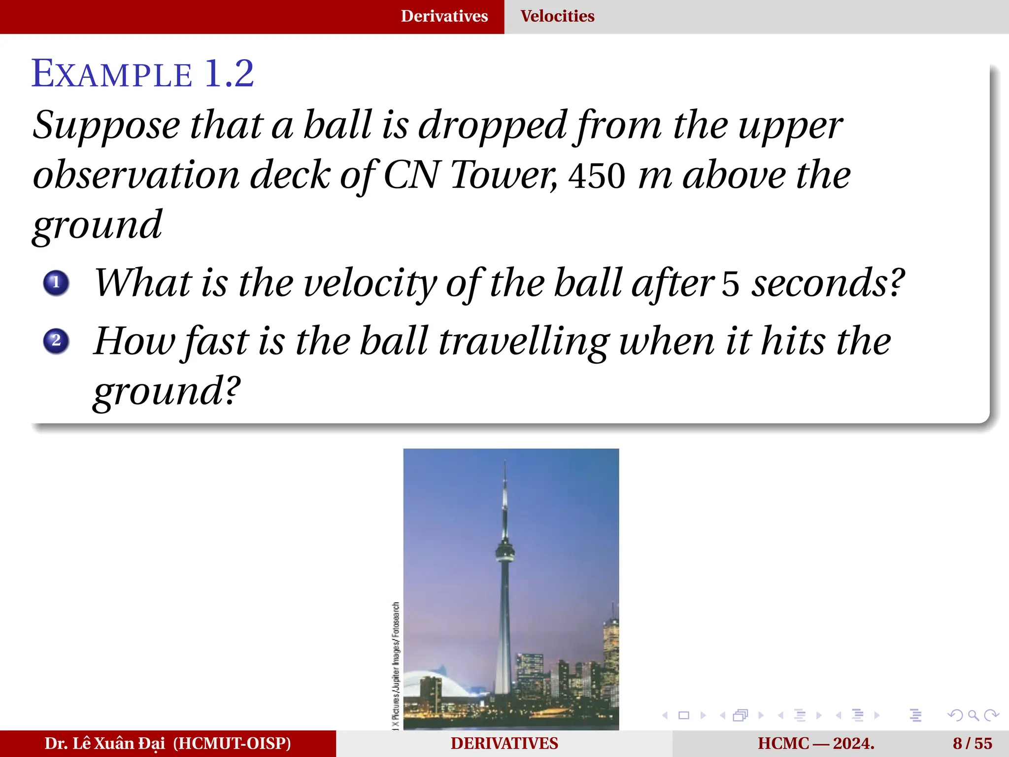
EXAMPLE 1.2
Supposethat a ball is dropped from the upper
observation deck of CN Tower, 450 m above the
ground
1
What is the velocity of the ball after 5 seconds?
Dr. Lê Xuân Đại (HCMUT-OISP) DERIVATIVES HCMC — 2024. 8 / 55
14.
Derivatives Velocities
EXAMPLE 1.2
Supposethat a ball is dropped from the upper
observation deck of CN Tower, 450 m above the
ground
1
What is the velocity of the ball after 5 seconds?
2
How fast is the ball travelling when it hits the
ground?
Dr. Lê Xuân Đại (HCMUT-OISP) DERIVATIVES HCMC — 2024. 8 / 55
15.
Derivatives Velocities
EXAMPLE 1.2
Supposethat a ball is dropped from the upper
observation deck of CN Tower, 450 m above the
ground
1
What is the velocity of the ball after 5 seconds?
2
How fast is the ball travelling when it hits the
ground?
Dr. Lê Xuân Đại (HCMUT-OISP) DERIVATIVES HCMC — 2024. 8 / 55
Derivatives Velocities
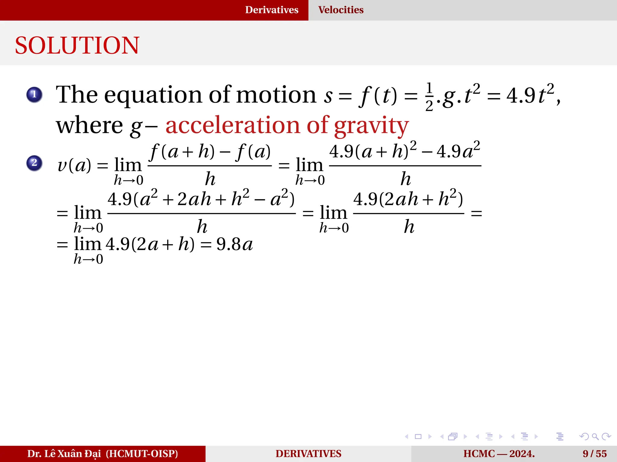
SOLUTION
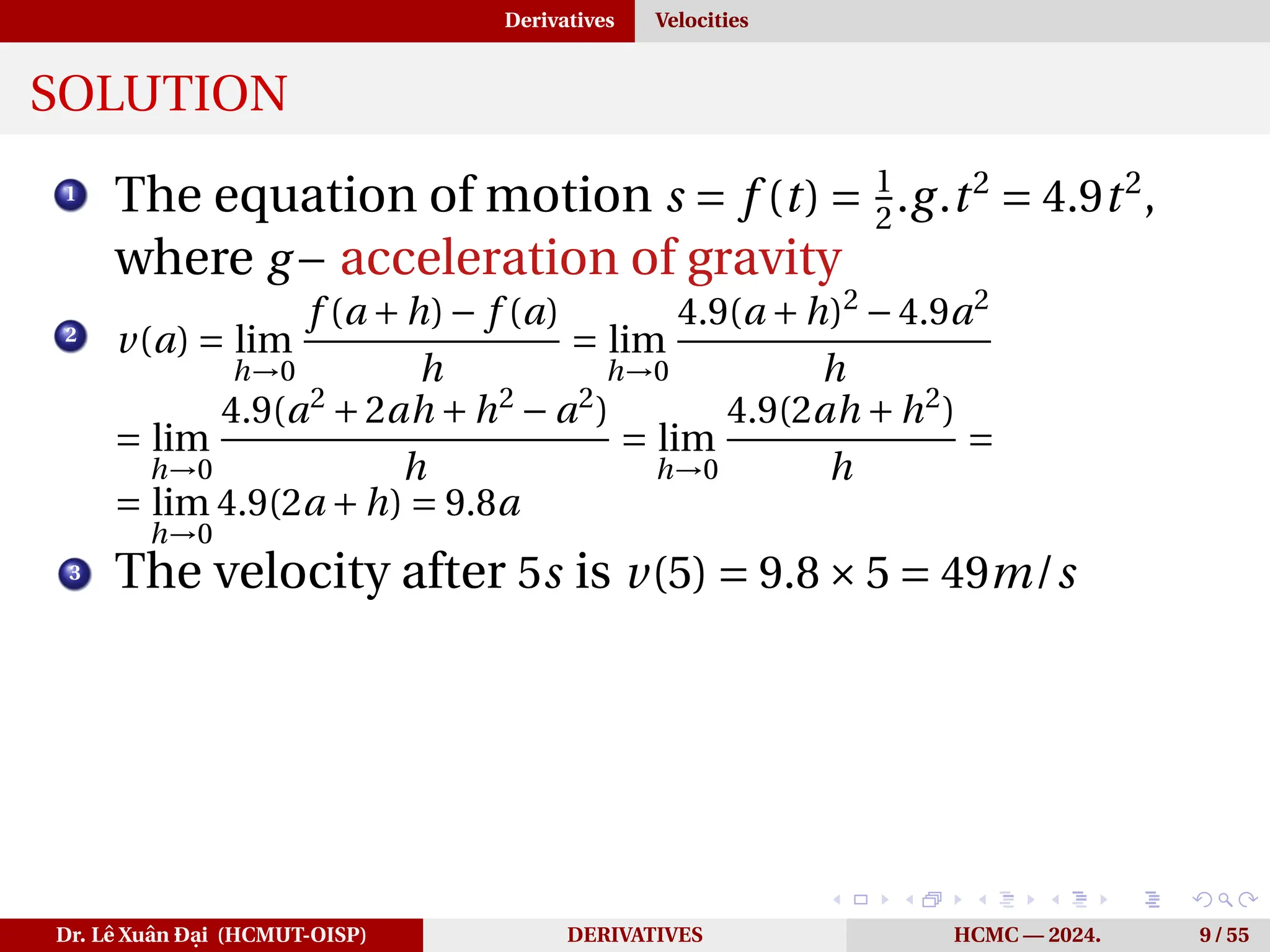
1
The equationof motion s = f (t) = 1
2
.g.t2
= 4.9t2
,
where g− acceleration of gravity
2
v(a) = lim
h→0
f (a +h)− f (a)
h
= lim
h→0
4.9(a +h)2
−4.9a2
h
= lim
h→0
4.9(a2
+2ah +h2
− a2
)
h
= lim
h→0
4.9(2ah +h2
)
h
=
= lim
h→0
4.9(2a +h) = 9.8a
Dr. Lê Xuân Đại (HCMUT-OISP) DERIVATIVES HCMC — 2024. 9 / 55
18.
Derivatives Velocities
SOLUTION
1
The equationof motion s = f (t) = 1
2
.g.t2
= 4.9t2
,
where g− acceleration of gravity
2
v(a) = lim
h→0
f (a +h)− f (a)
h
= lim
h→0
4.9(a +h)2
−4.9a2
h
= lim
h→0
4.9(a2
+2ah +h2
− a2
)
h
= lim
h→0
4.9(2ah +h2
)
h
=
= lim
h→0
4.9(2a +h) = 9.8a
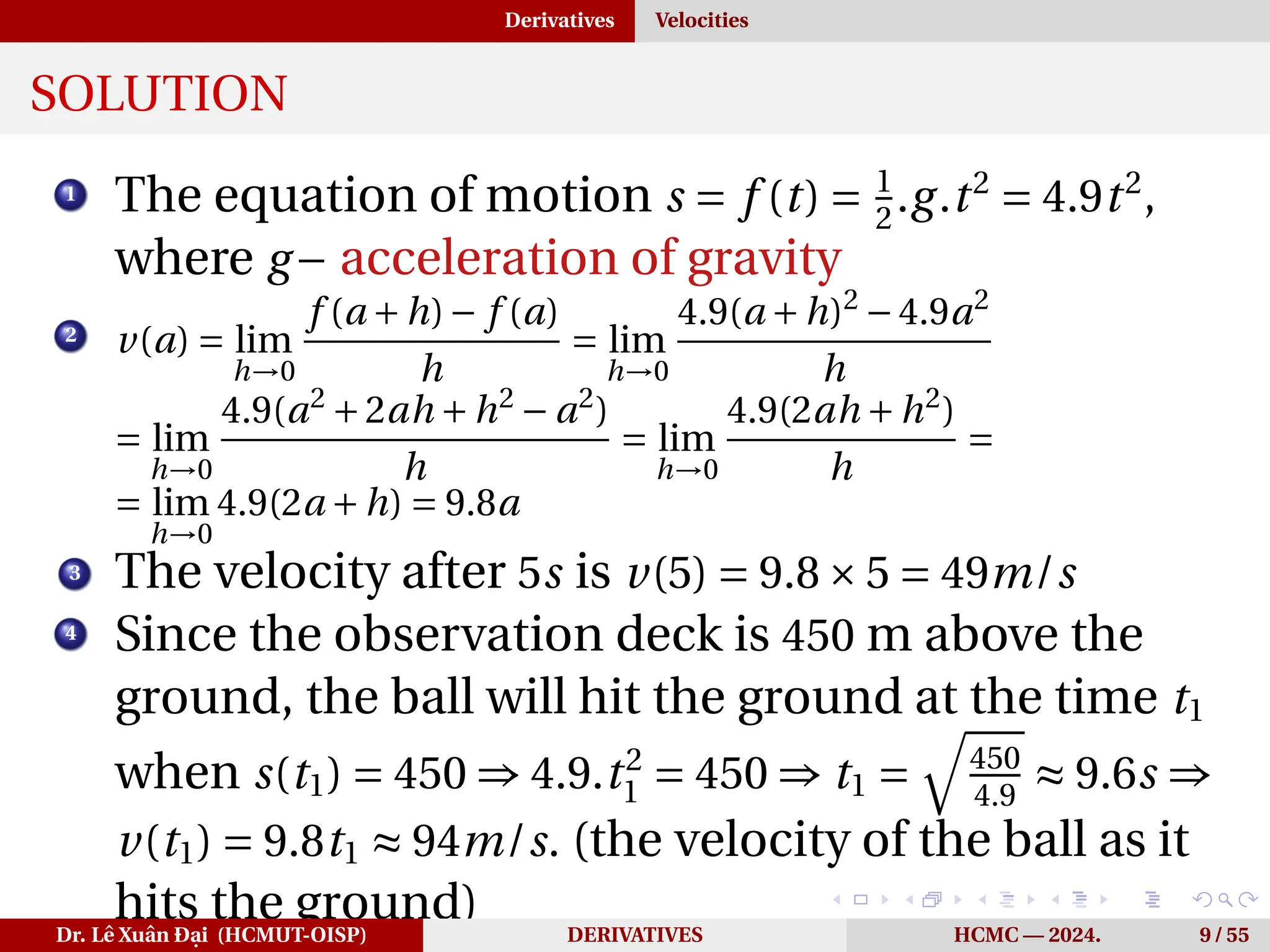
3 The velocity after 5s is v(5) = 9.8×5 = 49m/s
Dr. Lê Xuân Đại (HCMUT-OISP) DERIVATIVES HCMC — 2024. 9 / 55
19.
Derivatives Velocities
SOLUTION
1
The equationof motion s = f (t) = 1
2
.g.t2
= 4.9t2
,
where g− acceleration of gravity
2
v(a) = lim
h→0
f (a +h)− f (a)
h
= lim
h→0
4.9(a +h)2
−4.9a2
h
= lim
h→0
4.9(a2
+2ah +h2
− a2
)
h
= lim
h→0
4.9(2ah +h2
)
h
=
= lim
h→0
4.9(2a +h) = 9.8a
3 The velocity after 5s is v(5) = 9.8×5 = 49m/s
4
Since the observation deck is 450 m above the
ground, the ball will hit the ground at the time t1
when s(t1) = 450 ⇒ 4.9.t2
1 = 450 ⇒ t1 =
q
450
4.9
≈ 9.6s ⇒
v(t1) = 9.8t1 ≈ 94m/s. (the velocity of the ball as it
hits the ground)
Dr. Lê Xuân Đại (HCMUT-OISP) DERIVATIVES HCMC — 2024. 9 / 55
20.
Derivatives Definition
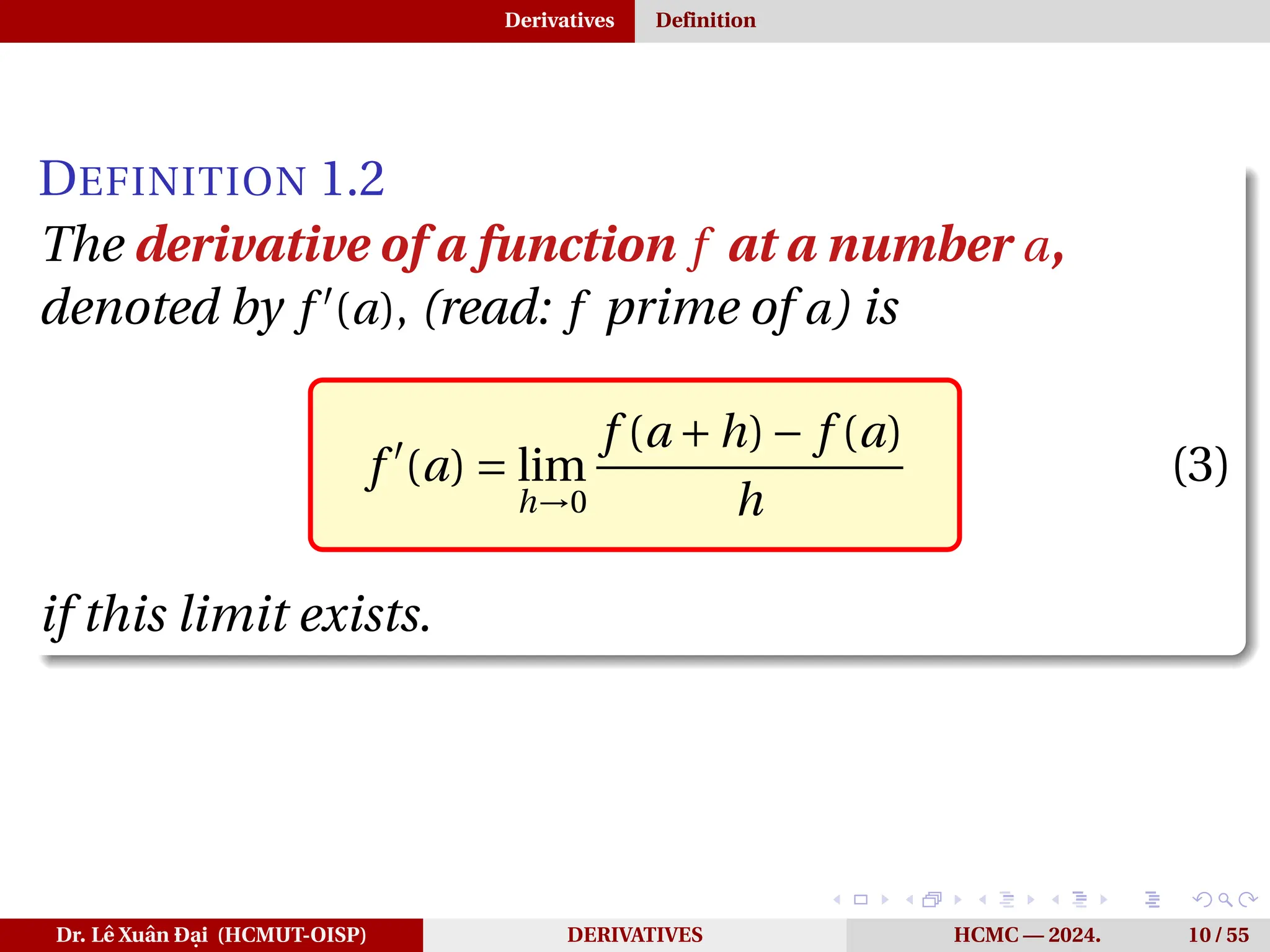
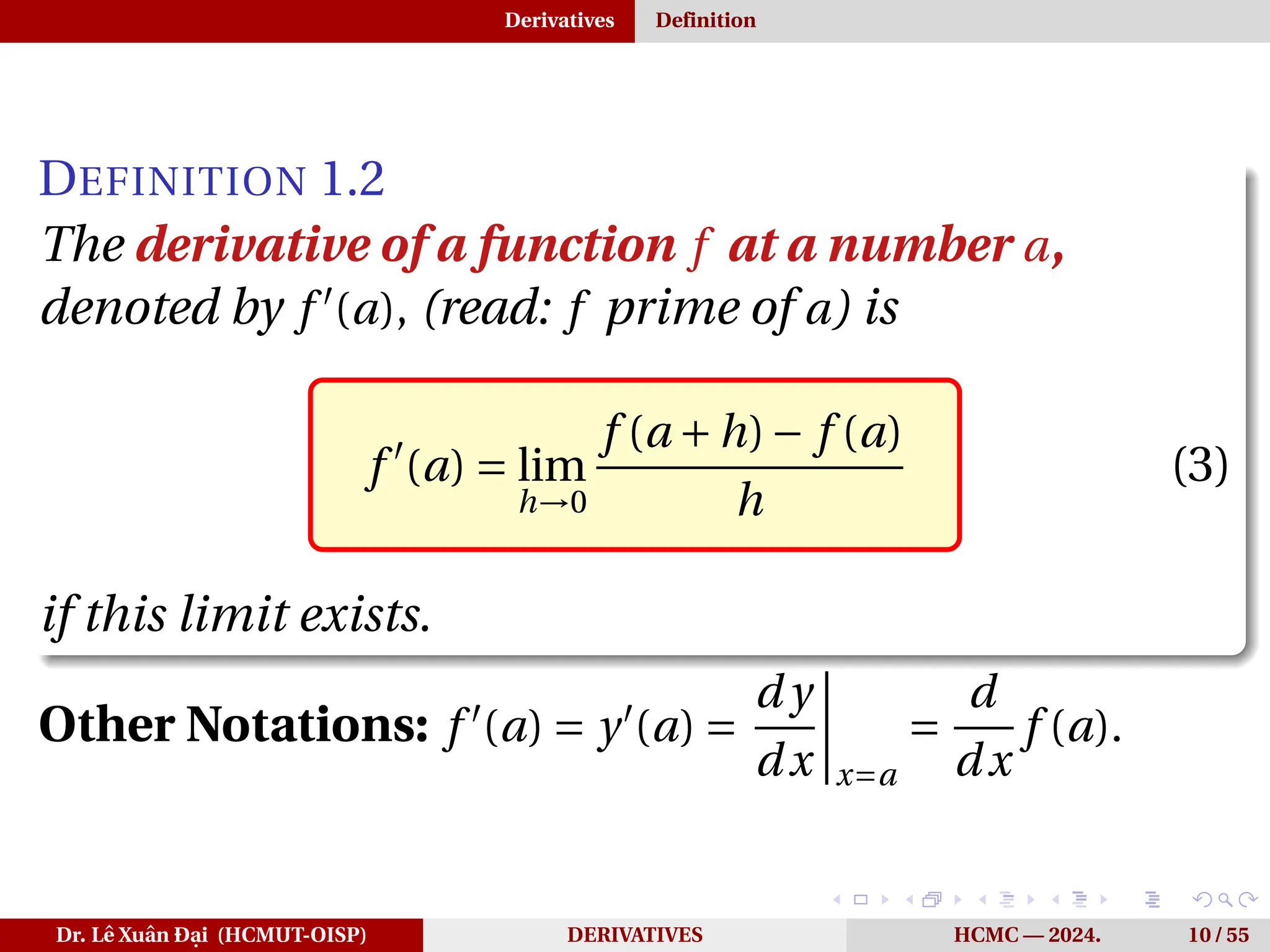
DEFINITION 1.2
Thederivative of a function f at a number a,
denoted by f ′
(a), (read: f prime of a) is
f ′
(a) = lim
h→0
f (a +h)− f (a)
h
(3)
if this limit exists.
Dr. Lê Xuân Đại (HCMUT-OISP) DERIVATIVES HCMC — 2024. 10 / 55
21.
Derivatives Definition
DEFINITION 1.2
Thederivative of a function f at a number a,
denoted by f ′
(a), (read: f prime of a) is
f ′
(a) = lim
h→0
f (a +h)− f (a)
h
(3)
if this limit exists.
Other Notations: f ′
(a) = y′
(a) =
d y
dx
¯
¯
¯
¯
x=a
=
d
dx
f (a).
Dr. Lê Xuân Đại (HCMUT-OISP) DERIVATIVES HCMC — 2024. 10 / 55
22.
Derivatives Definition
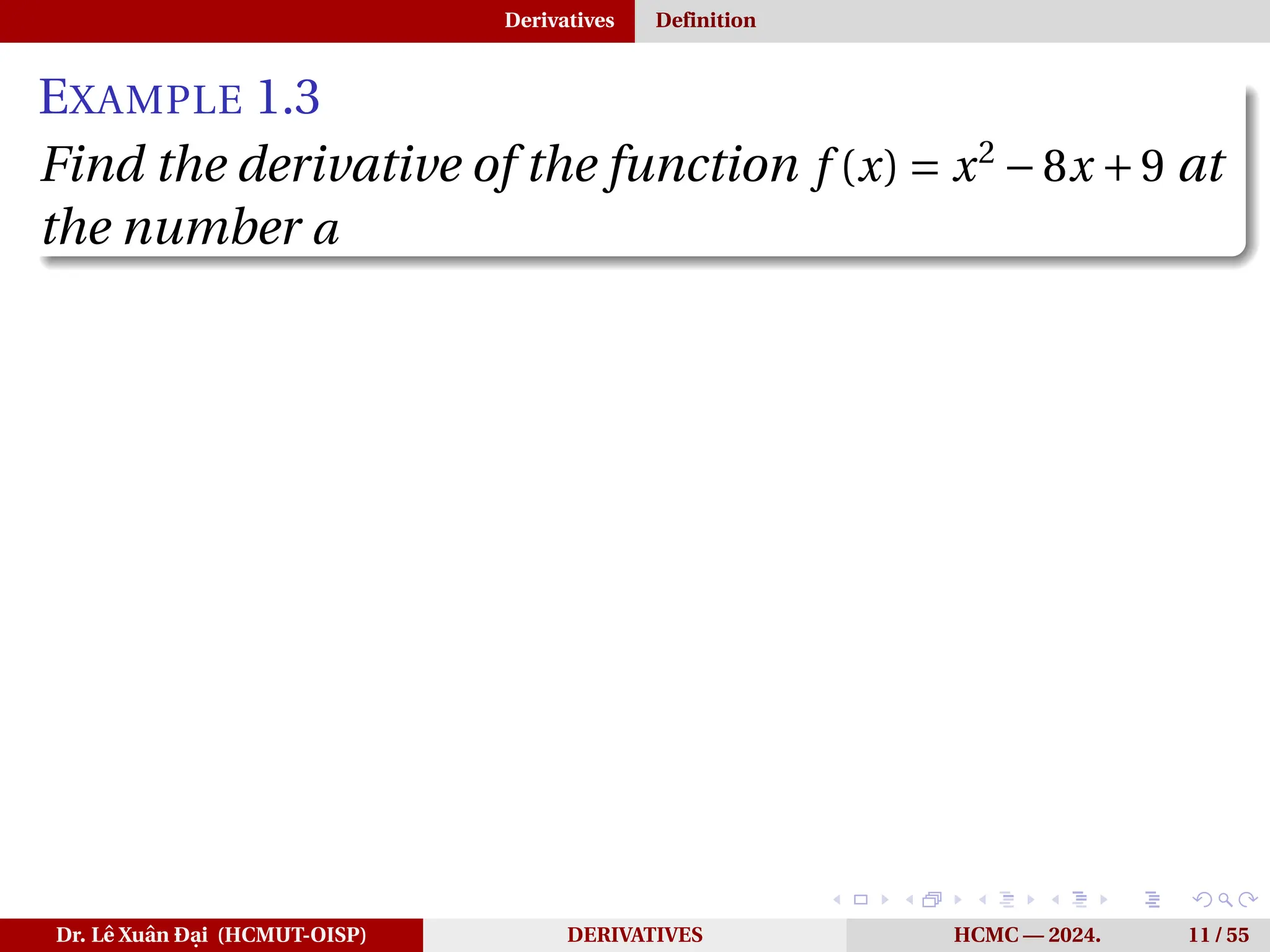
EXAMPLE 1.3
Findthe derivative of the function f (x) = x2
−8x +9 at
the number a
Dr. Lê Xuân Đại (HCMUT-OISP) DERIVATIVES HCMC — 2024. 11 / 55
23.
Derivatives Definition
EXAMPLE 1.3
Findthe derivative of the function f (x) = x2
−8x +9 at
the number a
SOLUTION
f ′
(a) = lim
h→0
f (a +h)− f (a)
h
=
= lim
h→0
[(a +h)2
−8(a +h)+9]−(a2
−8a +9)
h
=
= lim
h→0
a2
+2ah +h2
−8a −8h +9− a2
+8a −9
h
=
= lim
h→0
2ah +h2
−8h
h
= lim
h→0
(2a +h −8) = 2a −8
Dr. Lê Xuân Đại (HCMUT-OISP) DERIVATIVES HCMC — 2024. 11 / 55
24.
Derivatives Definition
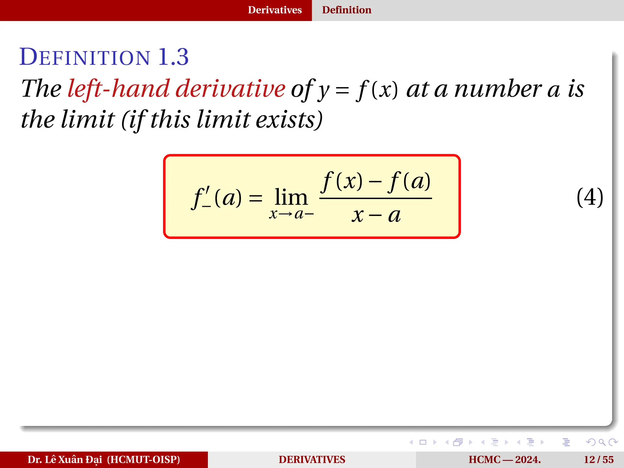
DEFINITION 1.3
Theleft-hand derivative of y = f (x) at a number a is
the limit (if this limit exists)
f ′
−(a) = lim
x→a−
f (x)− f (a)
x − a
(4)
Dr. Lê Xuân Đại (HCMUT-OISP) DERIVATIVES HCMC — 2024. 12 / 55
25.
Derivatives Definition
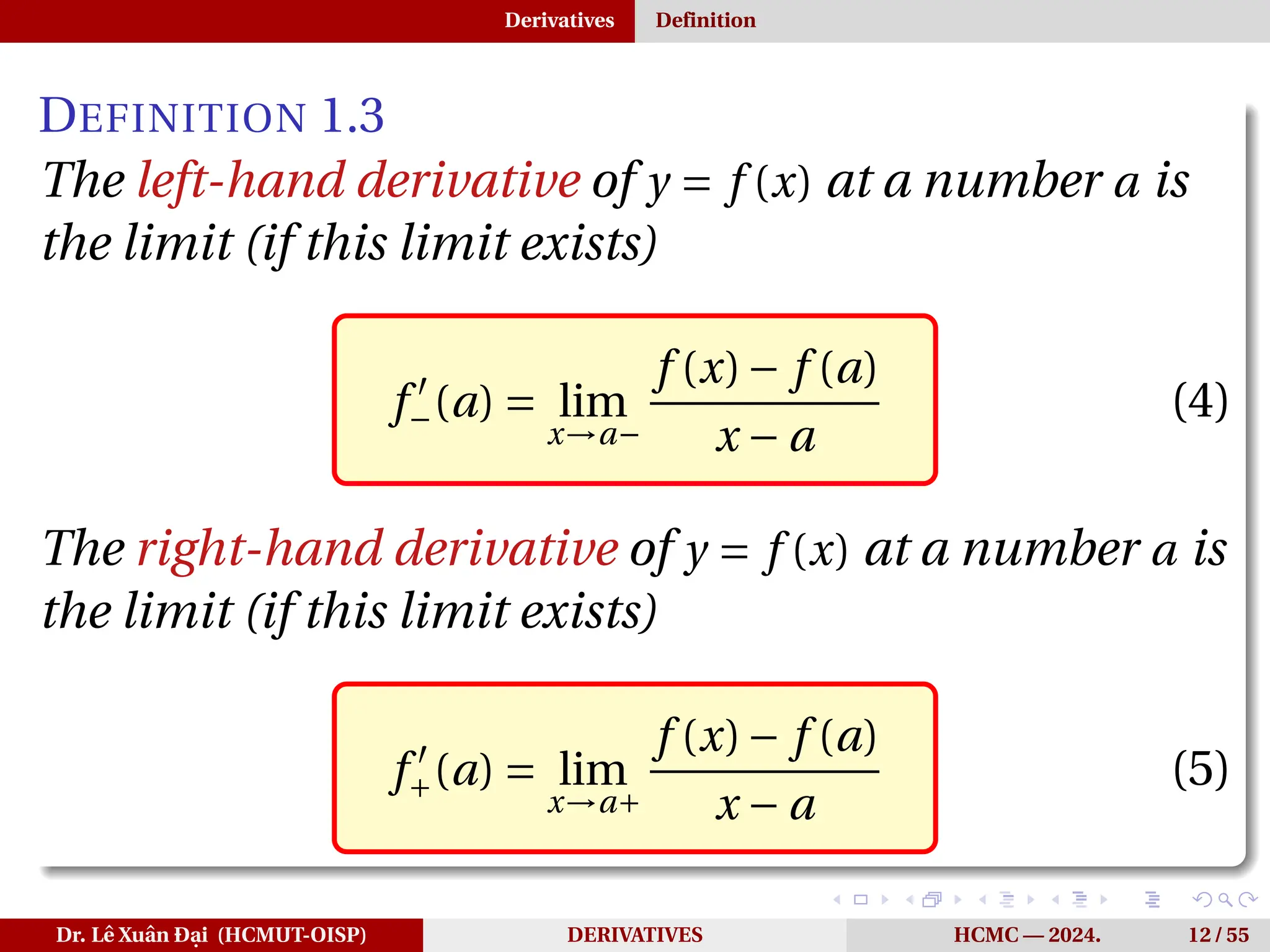
DEFINITION 1.3
Theleft-hand derivative of y = f (x) at a number a is
the limit (if this limit exists)
f ′
−(a) = lim
x→a−
f (x)− f (a)
x − a
(4)
The right-hand derivative of y = f (x) at a number a is
the limit (if this limit exists)
f ′
+(a) = lim
x→a+
f (x)− f (a)
x − a
(5)
Dr. Lê Xuân Đại (HCMUT-OISP) DERIVATIVES HCMC — 2024. 12 / 55
26.
Derivatives Definition
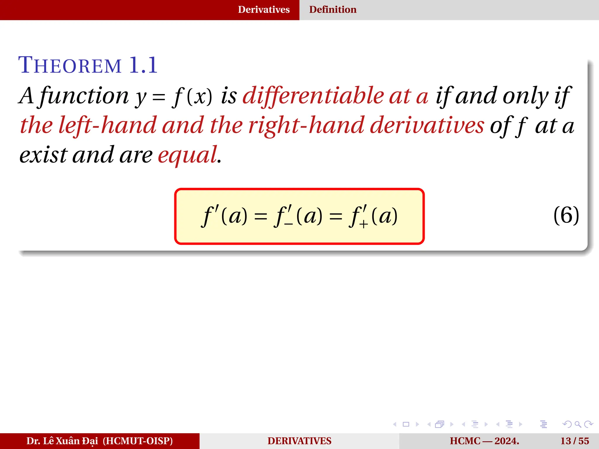
THEOREM 1.1
Afunction y = f (x) is differentiable at a if and only if
the left-hand and the right-hand derivatives of f at a
exist and are equal.
f ′
(a) = f ′
−(a) = f ′
+(a) (6)
Dr. Lê Xuân Đại (HCMUT-OISP) DERIVATIVES HCMC — 2024. 13 / 55
27.
Derivatives Definition
THEOREM 1.1
Afunction y = f (x) is differentiable at a if and only if
the left-hand and the right-hand derivatives of f at a
exist and are equal.
f ′
(a) = f ′
−(a) = f ′
+(a) (6)
DEFINITION 1.4
A function y = f (x) is differentiable on an open
interval (a,b) [or (a,∞) or (−∞,a) or (−∞,∞)] if it is
differentiable at every number in the interval.
Dr. Lê Xuân Đại (HCMUT-OISP) DERIVATIVES HCMC — 2024. 13 / 55
28.
Derivatives Definition
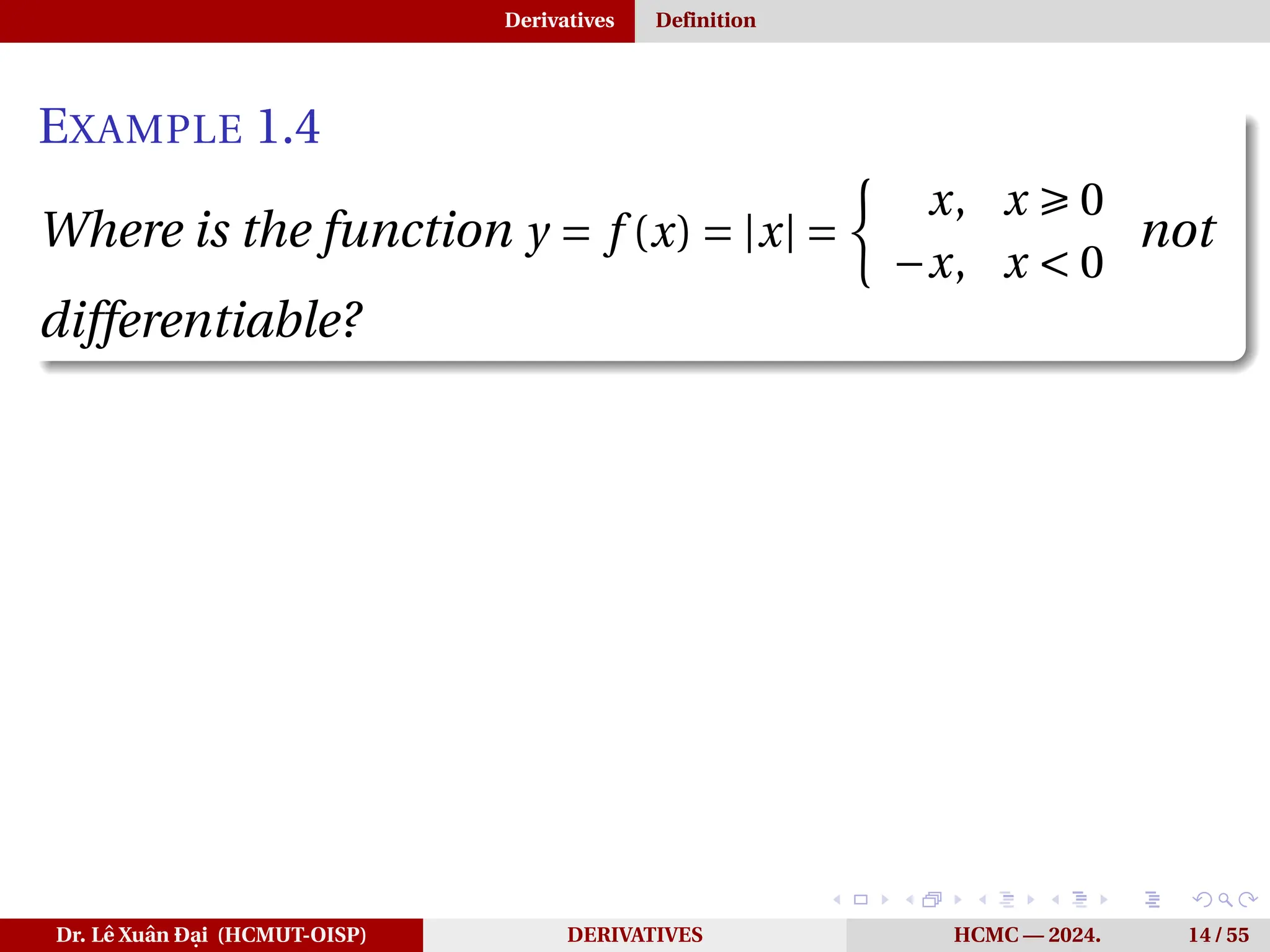
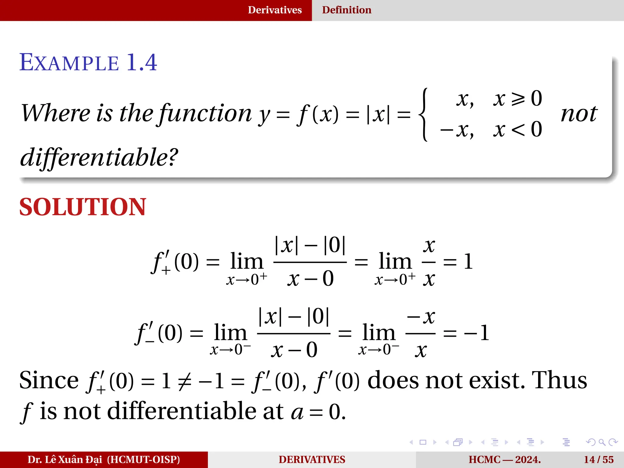
EXAMPLE 1.4
Whereis the function y = f (x) = |x| =
½
x, x Ê 0
−x, x < 0
not
differentiable?
Dr. Lê Xuân Đại (HCMUT-OISP) DERIVATIVES HCMC — 2024. 14 / 55
29.
Derivatives Definition
EXAMPLE 1.4
Whereis the function y = f (x) = |x| =
½
x, x Ê 0
−x, x < 0
not
differentiable?
SOLUTION
f ′
+(0) = lim
x→0+
|x|−|0|
x −0
= lim
x→0+
x
x
= 1
f ′
−(0) = lim
x→0−
|x|−|0|
x −0
= lim
x→0−
−x
x
= −1
Since f ′
+(0) = 1 ̸= −1 = f ′
−(0), f ′
(0) does not exist. Thus
f is not differentiable at a = 0.
Dr. Lê Xuân Đại (HCMUT-OISP) DERIVATIVES HCMC — 2024. 14 / 55
30.
Derivatives Definition
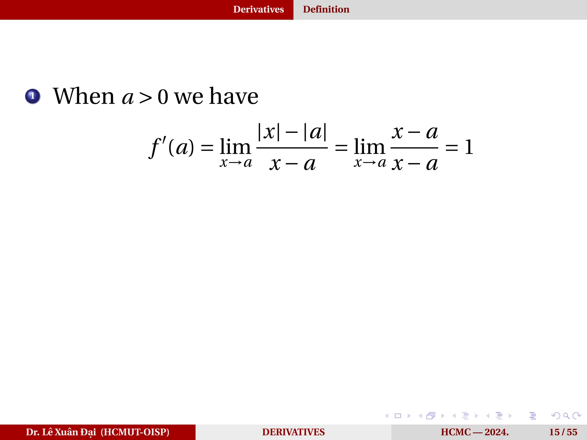
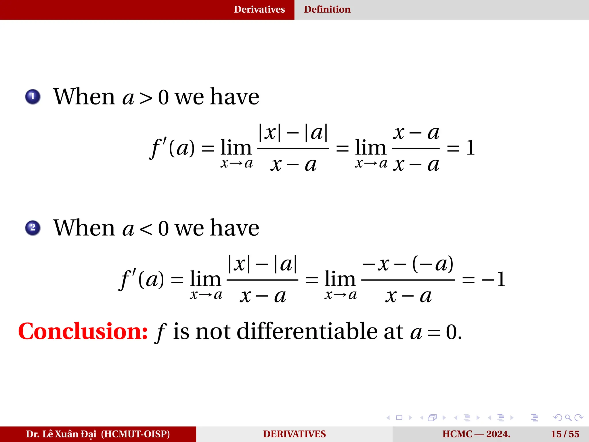
1
When a> 0 we have
f ′
(a) = lim
x→a
|x|−|a|
x − a
= lim
x→a
x − a
x − a
= 1
Dr. Lê Xuân Đại (HCMUT-OISP) DERIVATIVES HCMC — 2024. 15 / 55
31.
Derivatives Definition
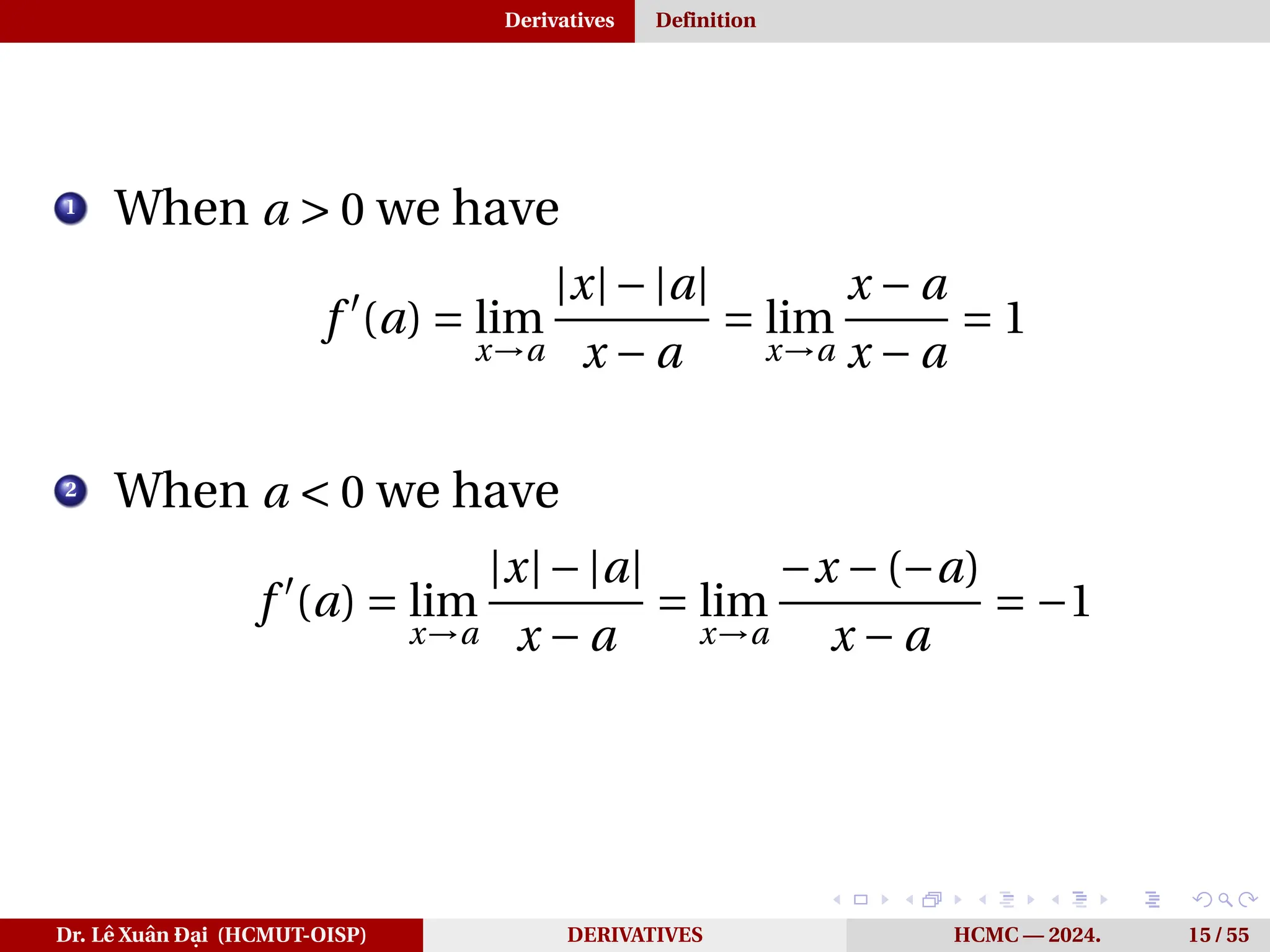
1
When a> 0 we have
f ′
(a) = lim
x→a
|x|−|a|
x − a
= lim
x→a
x − a
x − a
= 1
2
When a < 0 we have
f ′
(a) = lim
x→a
|x|−|a|
x − a
= lim
x→a
−x −(−a)
x − a
= −1
Dr. Lê Xuân Đại (HCMUT-OISP) DERIVATIVES HCMC — 2024. 15 / 55
32.
Derivatives Definition
1
When a> 0 we have
f ′
(a) = lim
x→a
|x|−|a|
x − a
= lim
x→a
x − a
x − a
= 1
2
When a < 0 we have
f ′
(a) = lim
x→a
|x|−|a|
x − a
= lim
x→a
−x −(−a)
x − a
= −1
Conclusion: f is not differentiable at a = 0.
Dr. Lê Xuân Đại (HCMUT-OISP) DERIVATIVES HCMC — 2024. 15 / 55
33.
Derivatives The derivativeof elementary functions
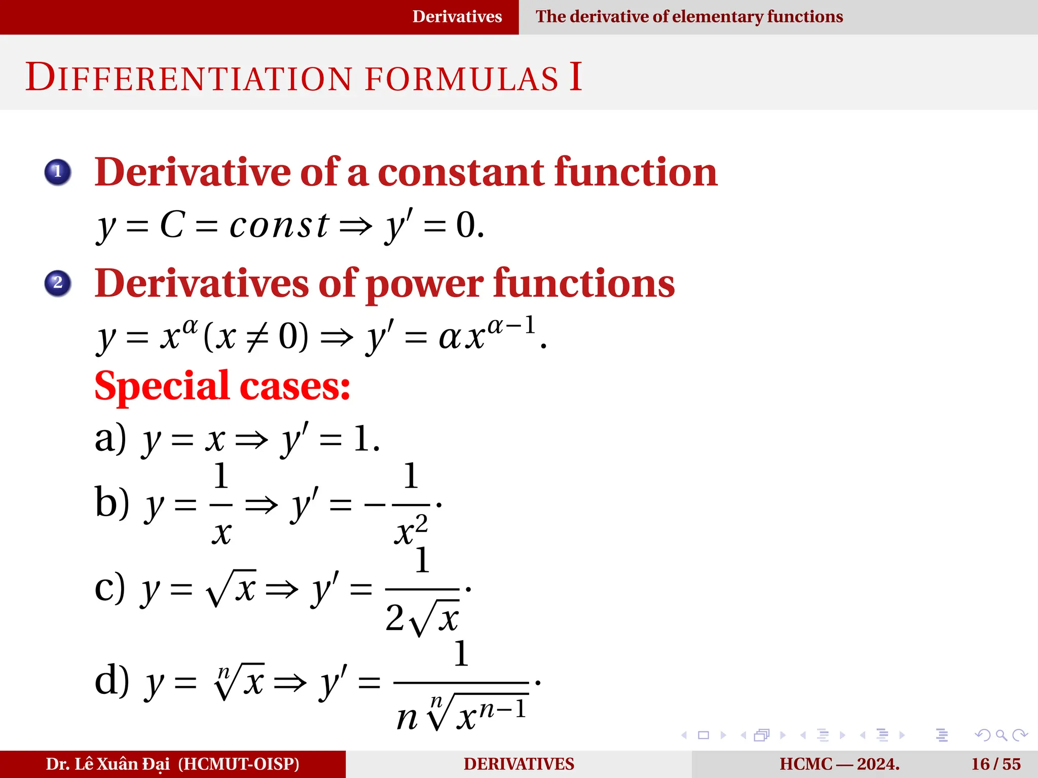
DIFFERENTIATION FORMULAS I
1
Derivative of a constant function
y = C = const ⇒ y′
= 0.
2
Derivatives of power functions
y = xα
(x ̸= 0) ⇒ y′
= αxα−1
.
Special cases:
a) y = x ⇒ y′
= 1.
b) y =
1
x
⇒ y′
= −
1
x2
·
c) y =
p
x ⇒ y′
=
1
2
p
x
·
d) y = n
p
x ⇒ y′
=
1
n
n
p
xn−1
·
Dr. Lê Xuân Đại (HCMUT-OISP) DERIVATIVES HCMC — 2024. 16 / 55
34.
Derivatives The derivativeof elementary functions
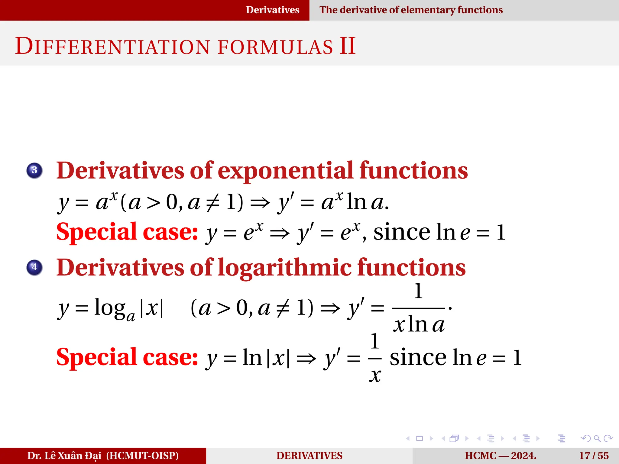
DIFFERENTIATION FORMULAS II
3
Derivatives of exponential functions
y = ax
(a > 0,a ̸= 1) ⇒ y′
= ax
lna.
Special case: y = ex
⇒ y′
= ex
, since lne = 1
4
Derivatives of logarithmic functions
y = loga |x| (a > 0,a ̸= 1) ⇒ y′
=
1
x lna
·
Special case: y = ln|x| ⇒ y′
=
1
x
since lne = 1
Dr. Lê Xuân Đại (HCMUT-OISP) DERIVATIVES HCMC — 2024. 17 / 55
35.
Derivatives The derivativeof elementary functions
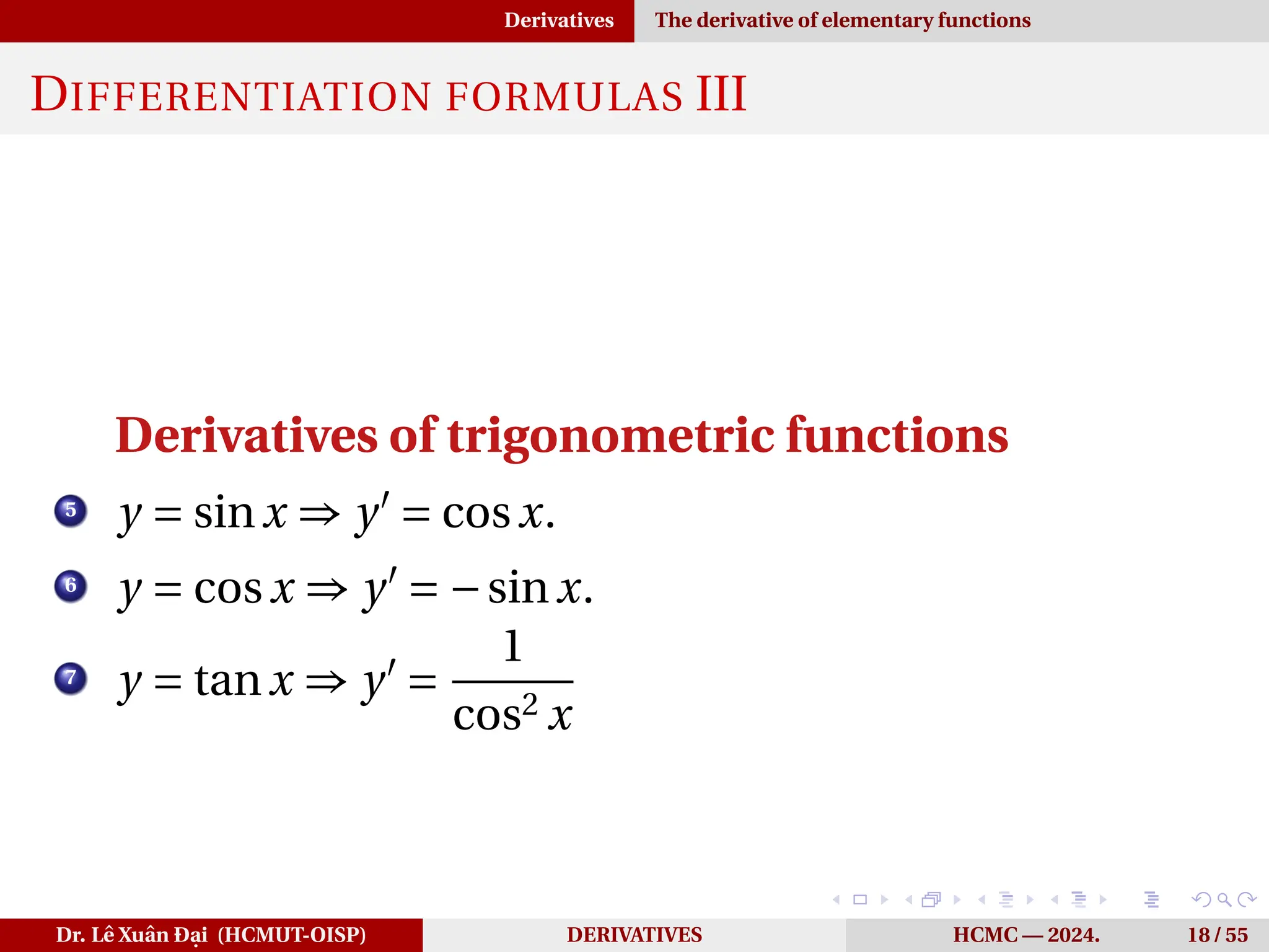
DIFFERENTIATION FORMULAS III
Derivatives of trigonometric functions
5
y = sinx ⇒ y′
= cosx.
6
y = cosx ⇒ y′
= −sinx.
7
y = tanx ⇒ y′
=
1
cos2 x
Dr. Lê Xuân Đại (HCMUT-OISP) DERIVATIVES HCMC — 2024. 18 / 55
36.
Derivatives The derivativeof elementary functions
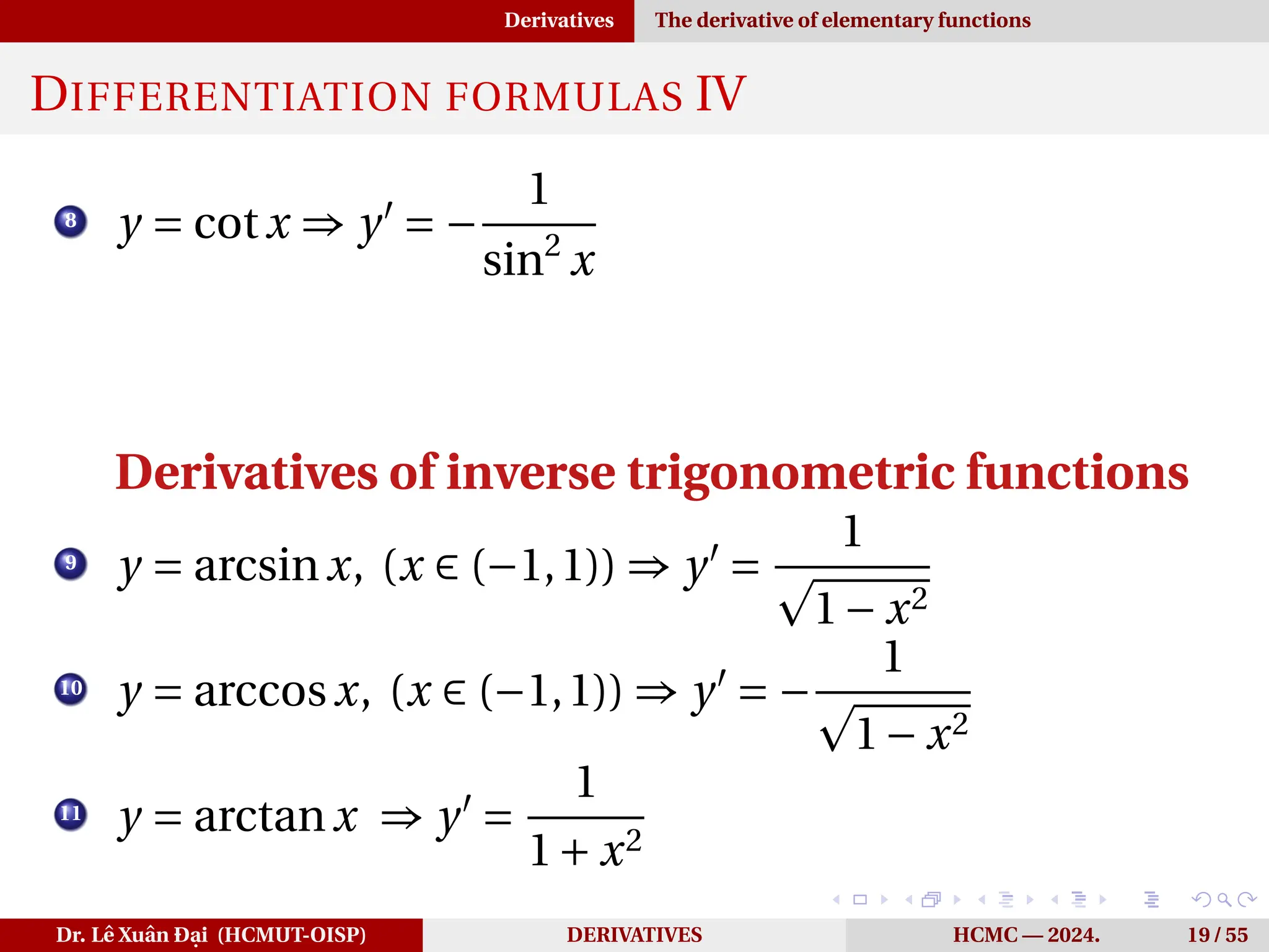
DIFFERENTIATION FORMULAS IV
8
y = cotx ⇒ y′
= −
1
sin2
x
Derivatives of inverse trigonometric functions
9
y = arcsinx, (x ∈ (−1,1)) ⇒ y′
=
1
p
1− x2
10
y = arccosx, (x ∈ (−1,1)) ⇒ y′
= −
1
p
1− x2
11
y = arctanx ⇒ y′
=
1
1+ x2
Dr. Lê Xuân Đại (HCMUT-OISP) DERIVATIVES HCMC — 2024. 19 / 55
37.
Derivatives The derivativeof elementary functions
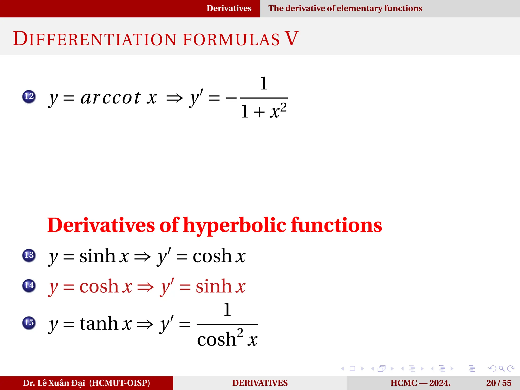
DIFFERENTIATION FORMULAS V
12
y = arccot x ⇒ y′
= −
1
1+ x2
Derivatives of hyperbolic functions
13
y = sinhx ⇒ y′
= coshx
14
y = coshx ⇒ y′
= sinhx
15
y = tanhx ⇒ y′
=
1
cosh2
x
Dr. Lê Xuân Đại (HCMUT-OISP) DERIVATIVES HCMC — 2024. 20 / 55
38.
Derivatives The derivativeof elementary functions
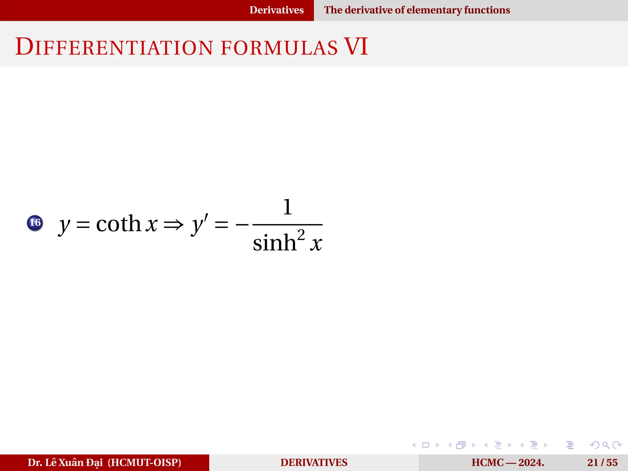
DIFFERENTIATION FORMULAS VI
16
y = cothx ⇒ y′
= −
1
sinh2
x
Dr. Lê Xuân Đại (HCMUT-OISP) DERIVATIVES HCMC — 2024. 21 / 55
39.
Derivatives Differentiation rules
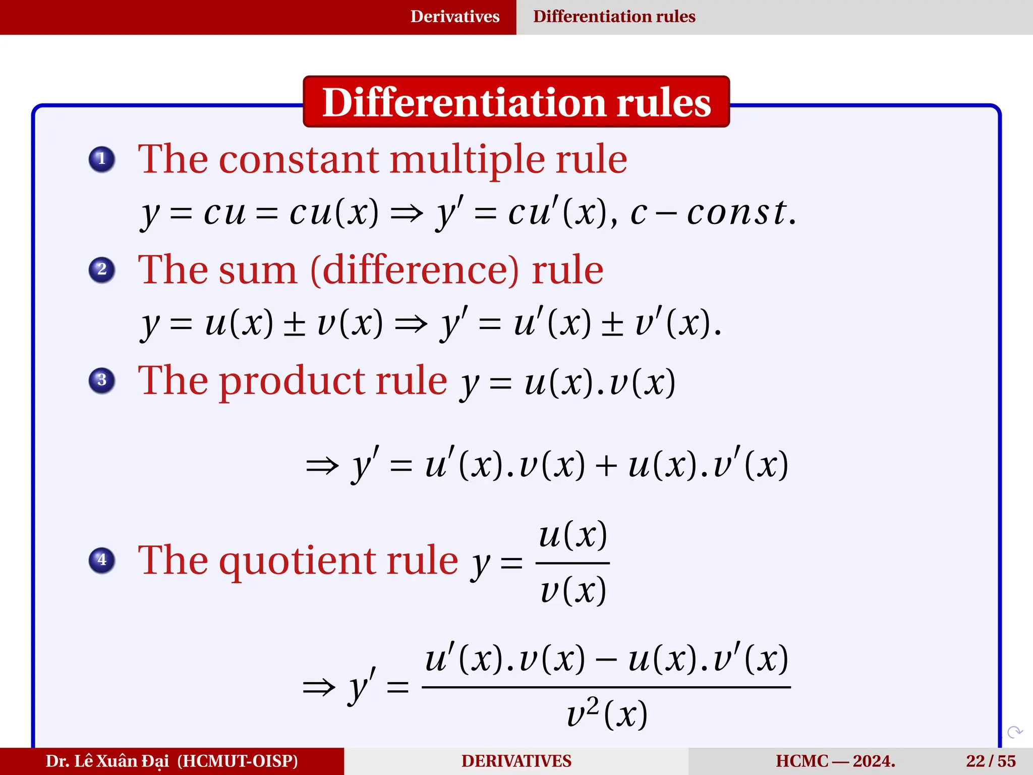
Differentiationrules
1
The constant multiple rule
y = cu = cu(x) ⇒ y′
= cu′
(x), c −const.
2
The sum (difference) rule
y = u(x)± v(x) ⇒ y′
= u′
(x)± v′
(x).
3
The product rule y = u(x).v(x)
⇒ y′
= u′
(x).v(x)+u(x).v′
(x)
4
The quotient rule y =
u(x)
v(x)
⇒ y′
=
u′
(x).v(x)−u(x).v′
(x)
v2(x)
Dr. Lê Xuân Đại (HCMUT-OISP) DERIVATIVES HCMC — 2024. 22 / 55
40.
Derivatives The chainrule
THE CHAIN RULE
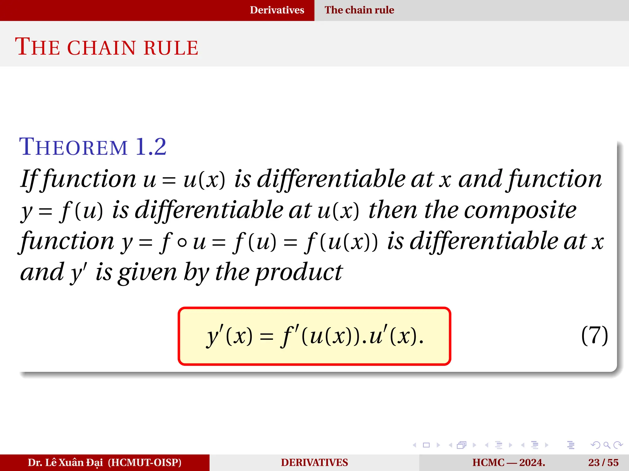
THEOREM 1.2
If function u = u(x) is differentiable at x and function
y = f (u) is differentiable at u(x) then the composite
function y = f ◦u = f (u) = f (u(x)) is differentiable at x
and y′
is given by the product
y′
(x) = f ′
(u(x)).u′
(x). (7)
Dr. Lê Xuân Đại (HCMUT-OISP) DERIVATIVES HCMC — 2024. 23 / 55
41.
Derivatives The chainrule
EXAMPLE 1.5
Differentiate y = sin5
(4x +3)
Dr. Lê Xuân Đại (HCMUT-OISP) DERIVATIVES HCMC — 2024. 24 / 55
42.
Derivatives The chainrule
EXAMPLE 1.5
Differentiate y = sin5
(4x +3)
SOLUTION
y′
= 5sin4
(4x +3).[sin(4x +3)]′
=
= 5sin4
(4x +3).cos(4x +3).(4x +3)′
=
= 20sin4
(4x +3)cos(4x +3).
Dr. Lê Xuân Đại (HCMUT-OISP) DERIVATIVES HCMC — 2024. 24 / 55
43.
Higher derivatives Thesecond derivative
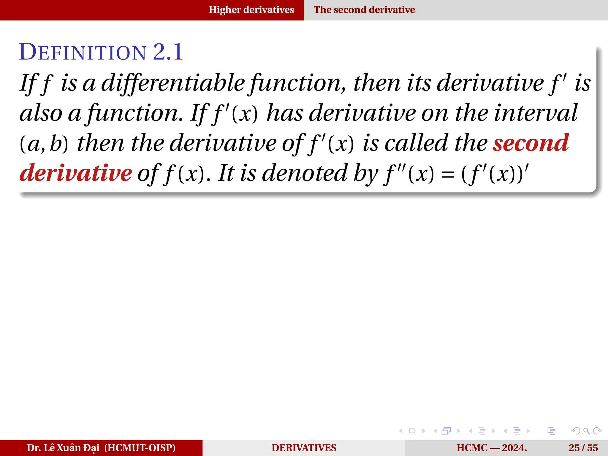
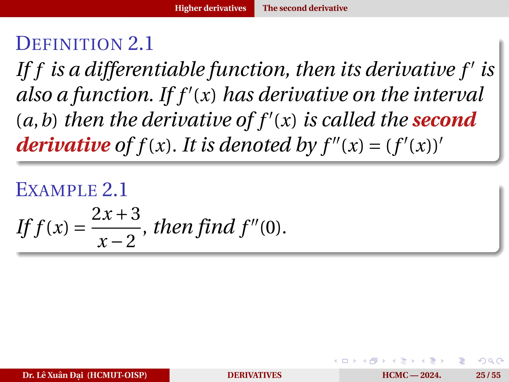
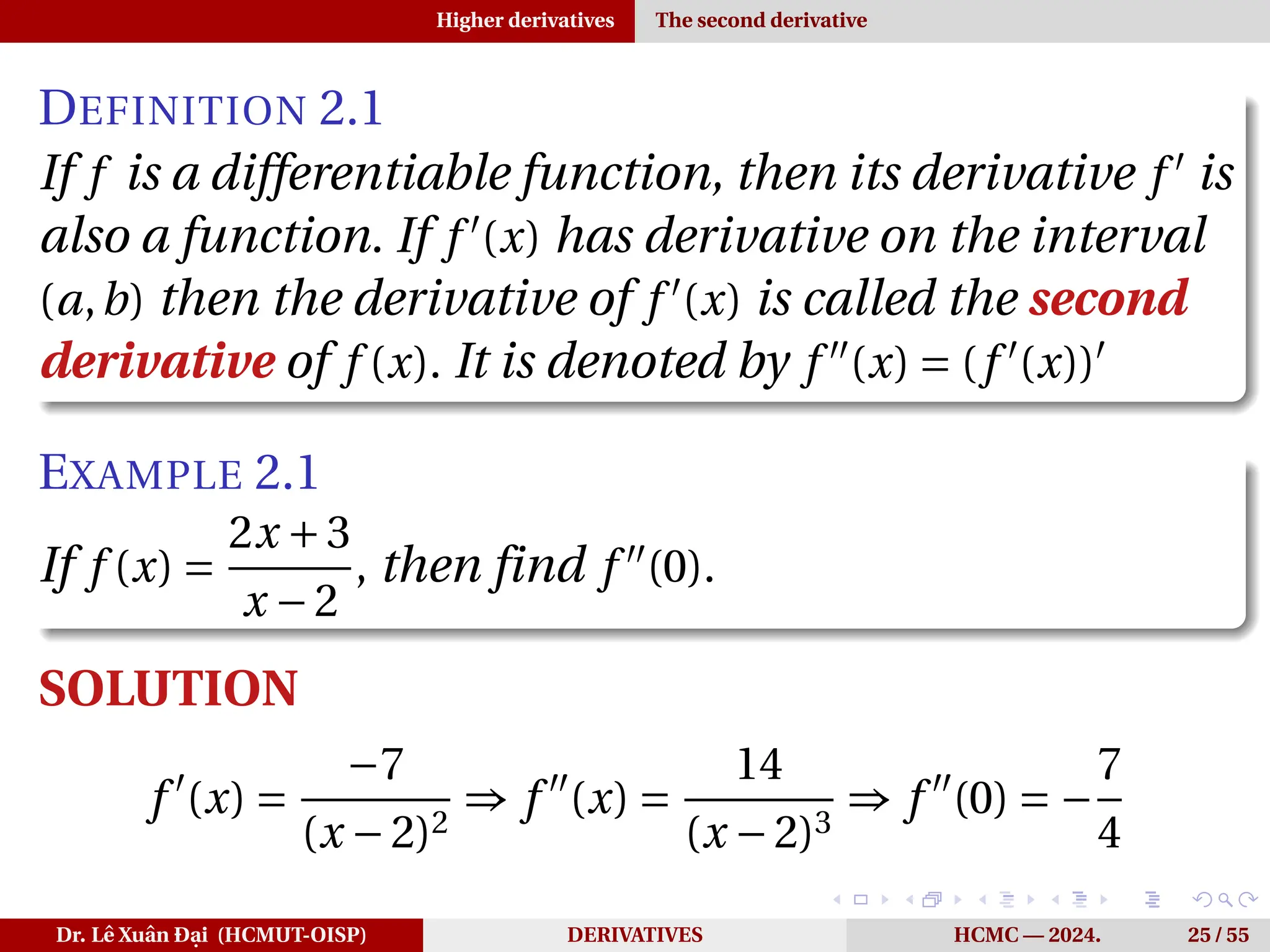
DEFINITION 2.1
If f is a differentiable function, then its derivative f ′
is
also a function. If f ′
(x) has derivative on the interval
(a,b) then the derivative of f ′
(x) is called the second
derivative of f (x). It is denoted by f ′′
(x) = (f ′
(x))′
Dr. Lê Xuân Đại (HCMUT-OISP) DERIVATIVES HCMC — 2024. 25 / 55
44.
Higher derivatives Thesecond derivative
DEFINITION 2.1
If f is a differentiable function, then its derivative f ′
is
also a function. If f ′
(x) has derivative on the interval
(a,b) then the derivative of f ′
(x) is called the second
derivative of f (x). It is denoted by f ′′
(x) = (f ′
(x))′
EXAMPLE 2.1
If f (x) =
2x +3
x −2
, then find f ′′
(0).
Dr. Lê Xuân Đại (HCMUT-OISP) DERIVATIVES HCMC — 2024. 25 / 55
45.
Higher derivatives Thesecond derivative
DEFINITION 2.1
If f is a differentiable function, then its derivative f ′
is
also a function. If f ′
(x) has derivative on the interval
(a,b) then the derivative of f ′
(x) is called the second
derivative of f (x). It is denoted by f ′′
(x) = (f ′
(x))′
EXAMPLE 2.1
If f (x) =
2x +3
x −2
, then find f ′′
(0).
SOLUTION
f ′
(x) =
−7
(x −2)2
⇒ f ′′
(x) =
14
(x −2)3
⇒ f ′′
(0) = −
7
4
Dr. Lê Xuân Đại (HCMUT-OISP) DERIVATIVES HCMC — 2024. 25 / 55
46.
Higher derivatives Thesecond derivative
EXAMPLE 2.2
If s = s(t) is the position function of an object that
moves in a straight line, we know that its first
derivative represents the velocity v(t) of the object as a
function of time:
v(t) = s′
(t)
The instantaneous rate of change of velocity with
respect to time is called the acceleration a(t) of the
object. Thus the acceleration function is the
derivative of the velocity function and is therefore the
second derivative of the position function:
a(t) = v′
(t) = s′′
(t)
Dr. Lê Xuân Đại (HCMUT-OISP) DERIVATIVES HCMC — 2024. 26 / 55
47.
Higher derivatives Then−th derivative
DEFINITION 2.2
The n−th derivative of f (x) is obtained from f by
differentiating n times.
f (n)
(x) = (f (n−1)
(x))′
, n ∈ N. (8)
Dr. Lê Xuân Đại (HCMUT-OISP) DERIVATIVES HCMC — 2024. 27 / 55
48.
Higher derivatives Then−th derivative
DEFINITION 2.2
The n−th derivative of f (x) is obtained from f by
differentiating n times.
f (n)
(x) = (f (n−1)
(x))′
, n ∈ N. (8)
PROPERTIES
If f (x) and g(x) have n−th derivatives then
c1 f (x)+c2g(x),c1,c2 ∈ R also has n−th derivative and
(c1 f (x)+c2g(x))(n)
= c1 f (n)
(x)+c2g(n)
(x) (9)
Dr. Lê Xuân Đại (HCMUT-OISP) DERIVATIVES HCMC — 2024. 27 / 55
49.
Higher derivatives Then−th derivative
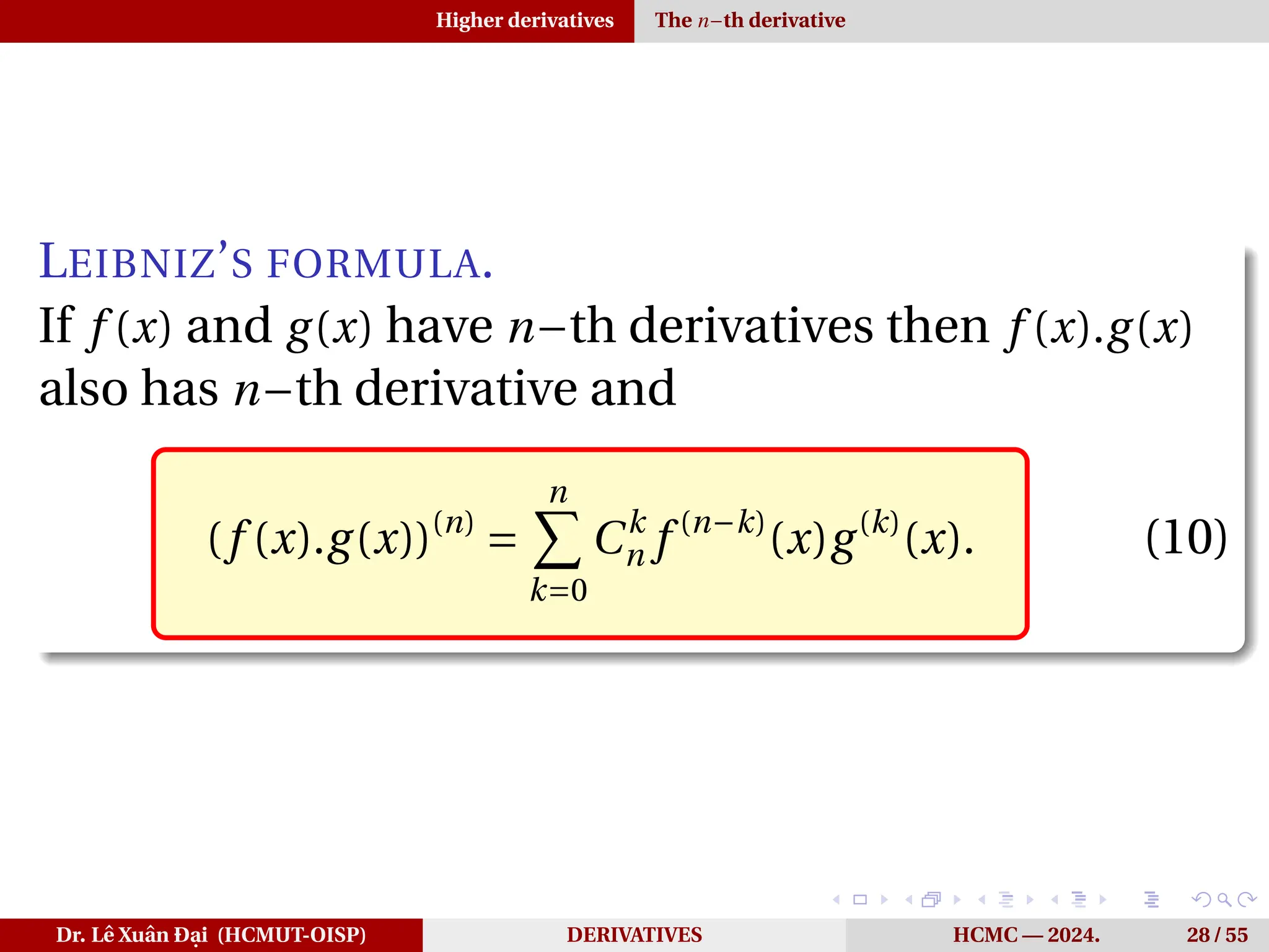
LEIBNIZ’S FORMULA.
If f (x) and g(x) have n−th derivatives then f (x).g(x)
also has n−th derivative and
(f (x).g(x))(n)
=
n
X
k=0
Ck
n f (n−k)
(x)g(k)
(x). (10)
Dr. Lê Xuân Đại (HCMUT-OISP) DERIVATIVES HCMC — 2024. 28 / 55
50.
Higher derivatives Somebasic formulas
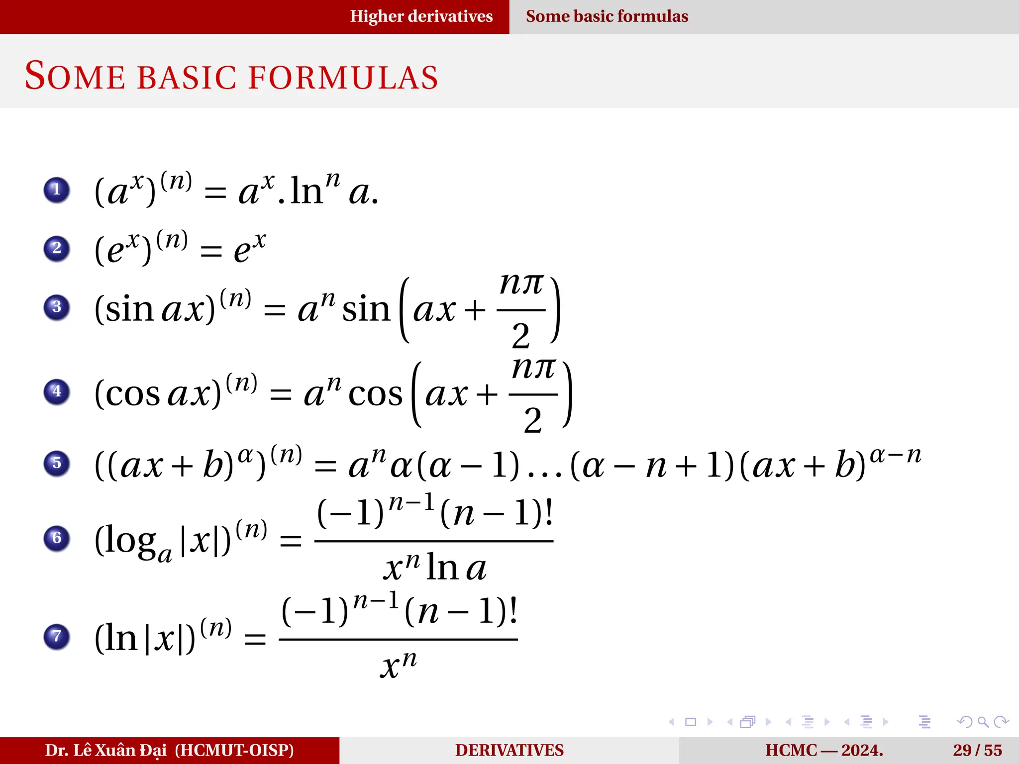
SOME BASIC FORMULAS
1
(ax
)(n)
= ax
.lnn
a.
2
(ex
)(n)
= ex
3
(sinax)(n)
= an
sin
³
ax +
nπ
2
´
4
(cosax)(n)
= an
cos
³
ax +
nπ
2
´
5
((ax +b)α
)(n)
= an
α(α−1)...(α−n +1)(ax +b)α−n
6
(loga |x|)(n)
=
(−1)n−1
(n −1)!
xn lna
7
(ln|x|)(n)
=
(−1)n−1
(n −1)!
xn
Dr. Lê Xuân Đại (HCMUT-OISP) DERIVATIVES HCMC — 2024. 29 / 55
51.
Higher derivatives Somebasic formulas
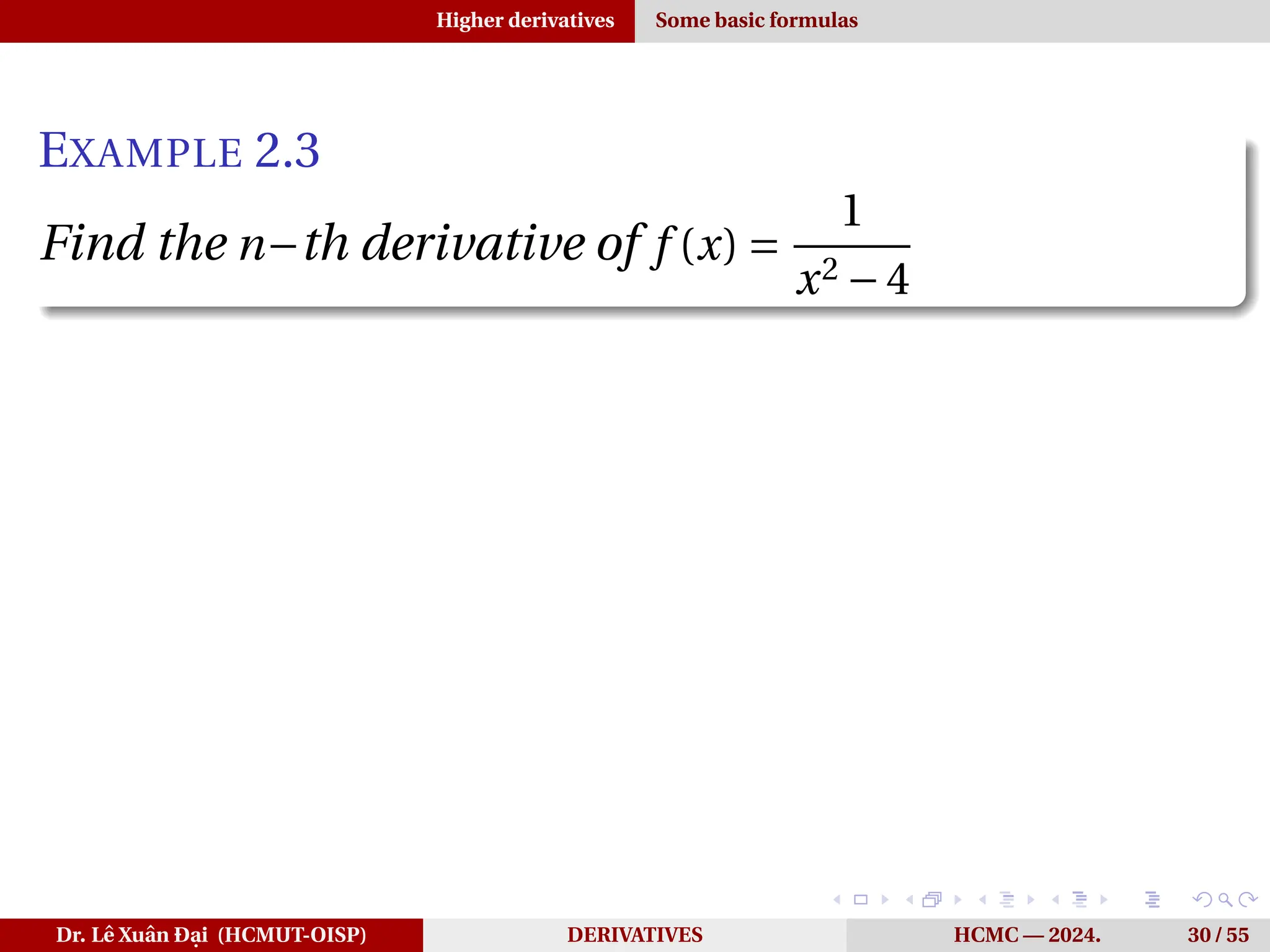
EXAMPLE 2.3
Find the n−th derivative of f (x) =
1
x2 −4
Dr. Lê Xuân Đại (HCMUT-OISP) DERIVATIVES HCMC — 2024. 30 / 55
52.
Higher derivatives Somebasic formulas
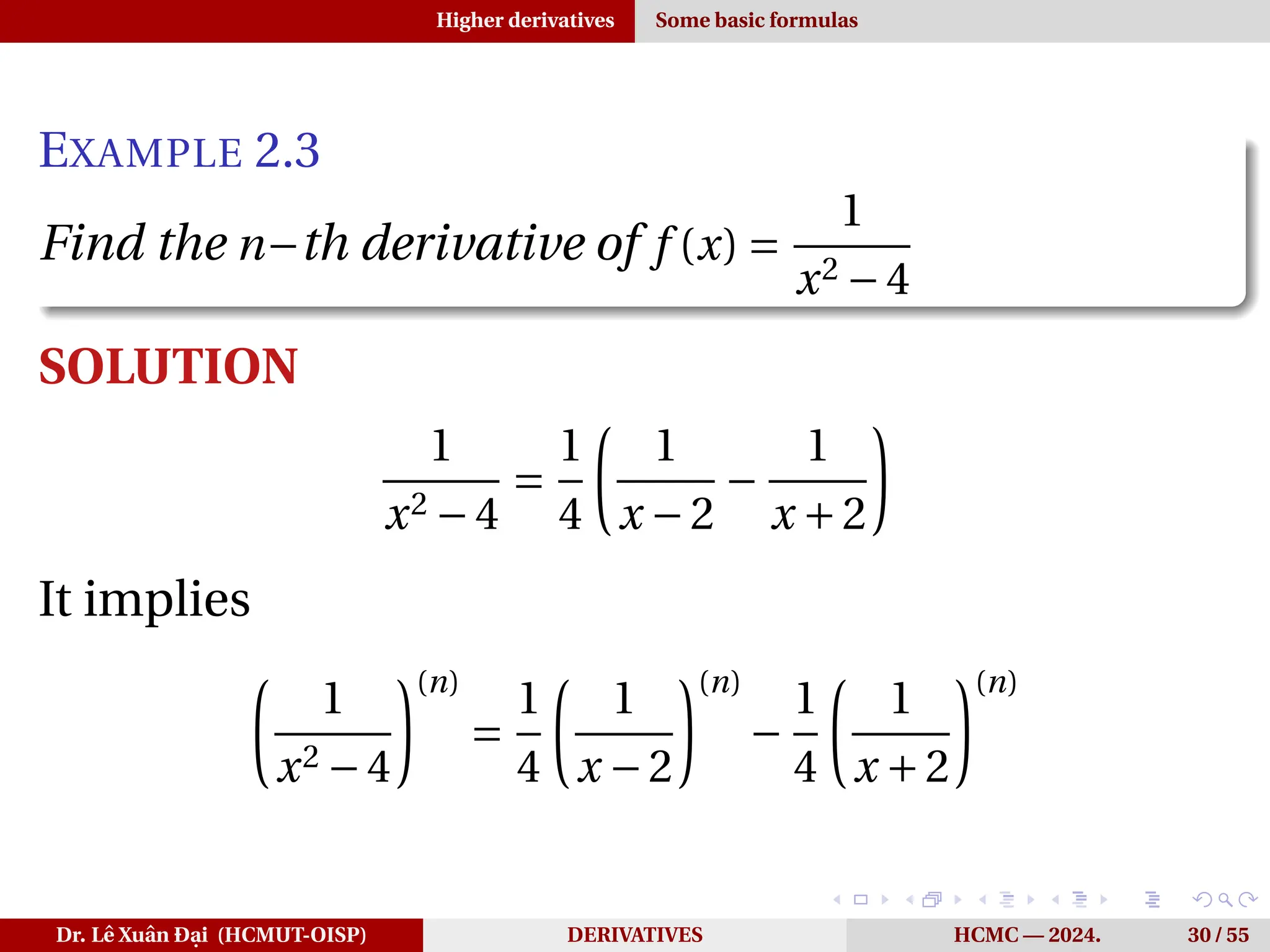
EXAMPLE 2.3
Find the n−th derivative of f (x) =
1
x2 −4
SOLUTION
1
x2 −4
=
1
4
µ
1
x −2
−
1
x +2
It implies
µ
1
x2 −4
¶(n)
=
1
4
µ
1
x −2
¶(n)
−
1
4
µ
1
x +2
¶(n)
Dr. Lê Xuân Đại (HCMUT-OISP) DERIVATIVES HCMC — 2024. 30 / 55
53.
Higher derivatives Somebasic formulas
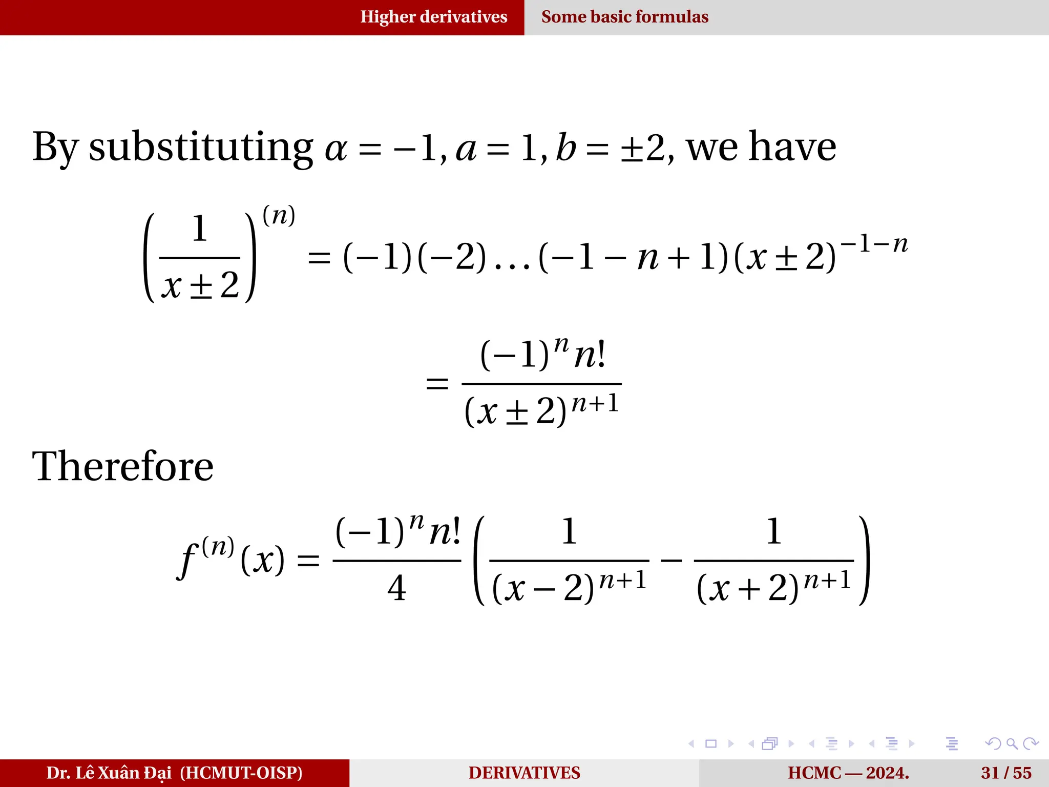
By substituting α = −1,a = 1,b = ±2, we have
µ
1
x ±2
¶(n)
= (−1)(−2)...(−1−n +1)(x ±2)−1−n
=
(−1)n
n!
(x ±2)n+1
Therefore
f (n)
(x) =
(−1)n
n!
4
µ
1
(x −2)n+1
−
1
(x +2)n+1
Dr. Lê Xuân Đại (HCMUT-OISP) DERIVATIVES HCMC — 2024. 31 / 55
54.
Higher derivatives Somebasic formulas
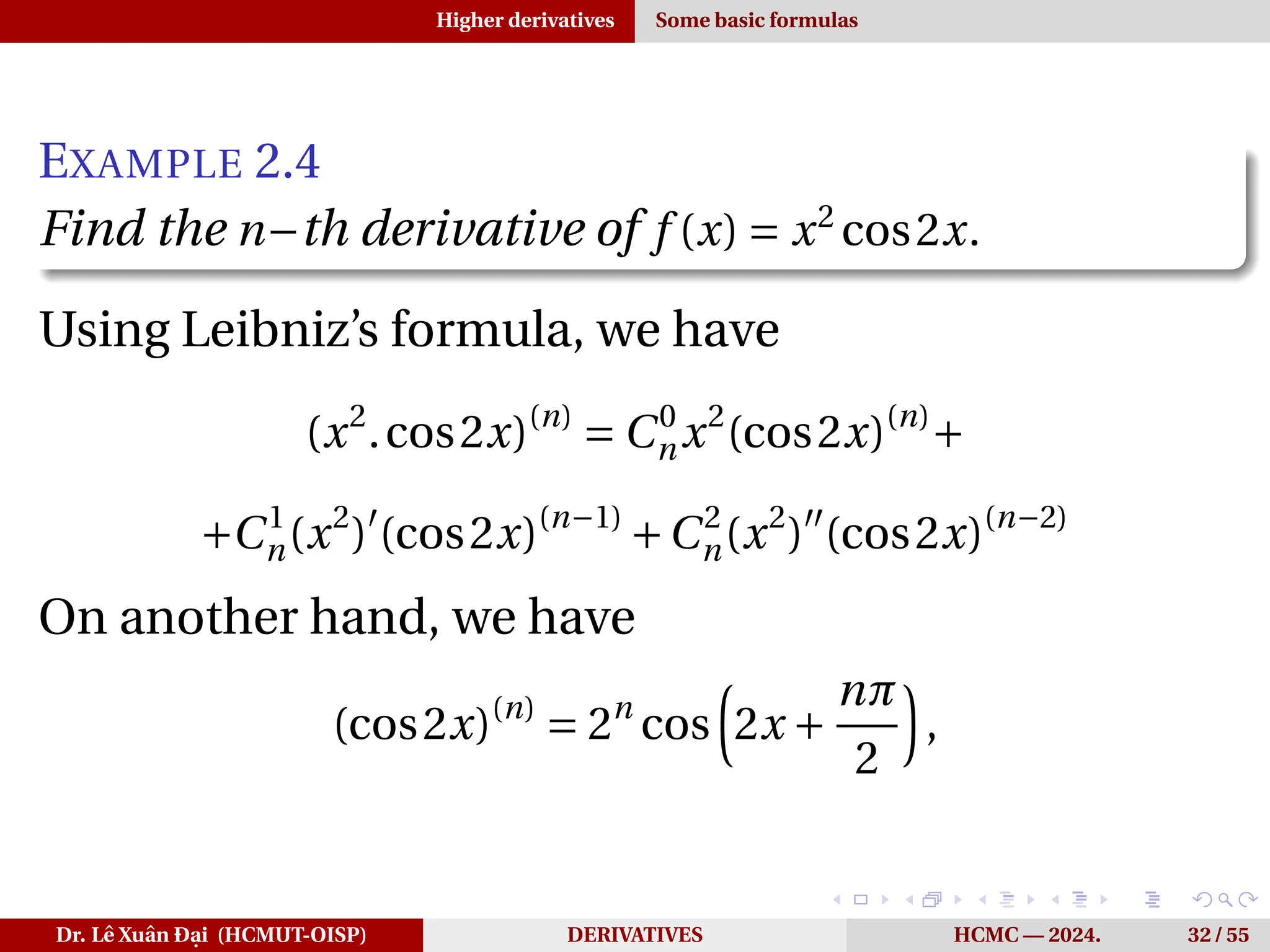
EXAMPLE 2.4
Find the n−th derivative of f (x) = x2
cos2x.
Dr. Lê Xuân Đại (HCMUT-OISP) DERIVATIVES HCMC — 2024. 32 / 55
55.
Higher derivatives Somebasic formulas
EXAMPLE 2.4
Find the n−th derivative of f (x) = x2
cos2x.
Using Leibniz’s formula, we have
(x2
.cos2x)(n)
= C0
nx2
(cos2x)(n)
+
+C1
n(x2
)′
(cos2x)(n−1)
+C2
n(x2
)′′
(cos2x)(n−2)
On another hand, we have
(cos2x)(n)
= 2n
cos
³
2x +
nπ
2
´
,
Dr. Lê Xuân Đại (HCMUT-OISP) DERIVATIVES HCMC — 2024. 32 / 55
56.
Higher derivatives Somebasic formulas
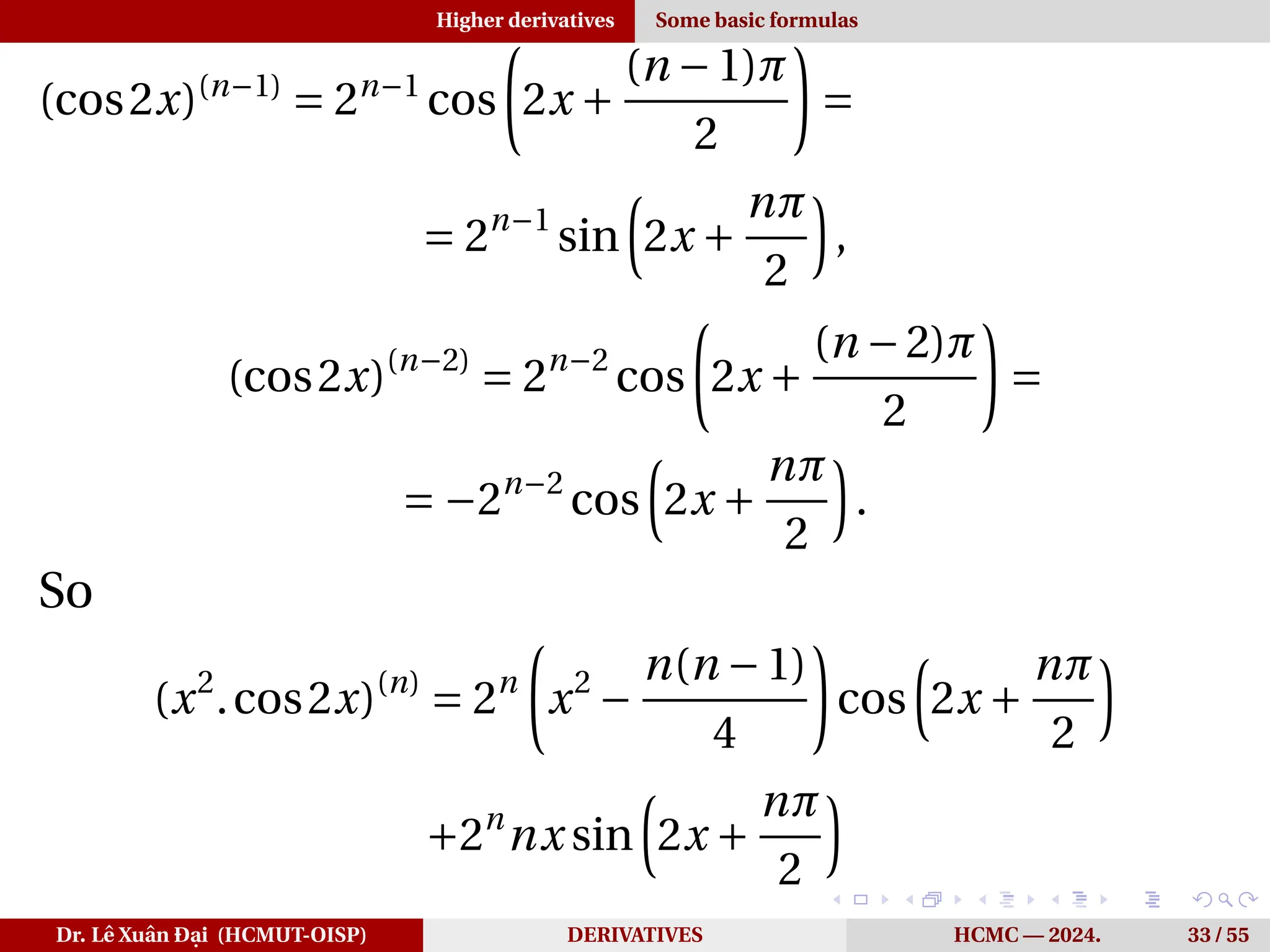
(cos2x)(n−1)
= 2n−1
cos
µ
2x +
(n −1)π
2
=
= 2n−1
sin
³
2x +
nπ
2
´
,
(cos2x)(n−2)
= 2n−2
cos
µ
2x +
(n −2)π
2
=
= −2n−2
cos
³
2x +
nπ
2
´
.
So
(x2
.cos2x)(n)
= 2n
µ
x2
−
n(n −1)
4
cos
³
2x +
nπ
2
´
+2n
nx sin
³
2x +
nπ
2
´
Dr. Lê Xuân Đại (HCMUT-OISP) DERIVATIVES HCMC — 2024. 33 / 55
57.
Linear approximations andDifferentials Linear approximations
LINEAR APPROXIMATIONS
Dr. Lê Xuân Đại (HCMUT-OISP) DERIVATIVES HCMC — 2024. 34 / 55
58.
Linear approximations andDifferentials Linear approximations
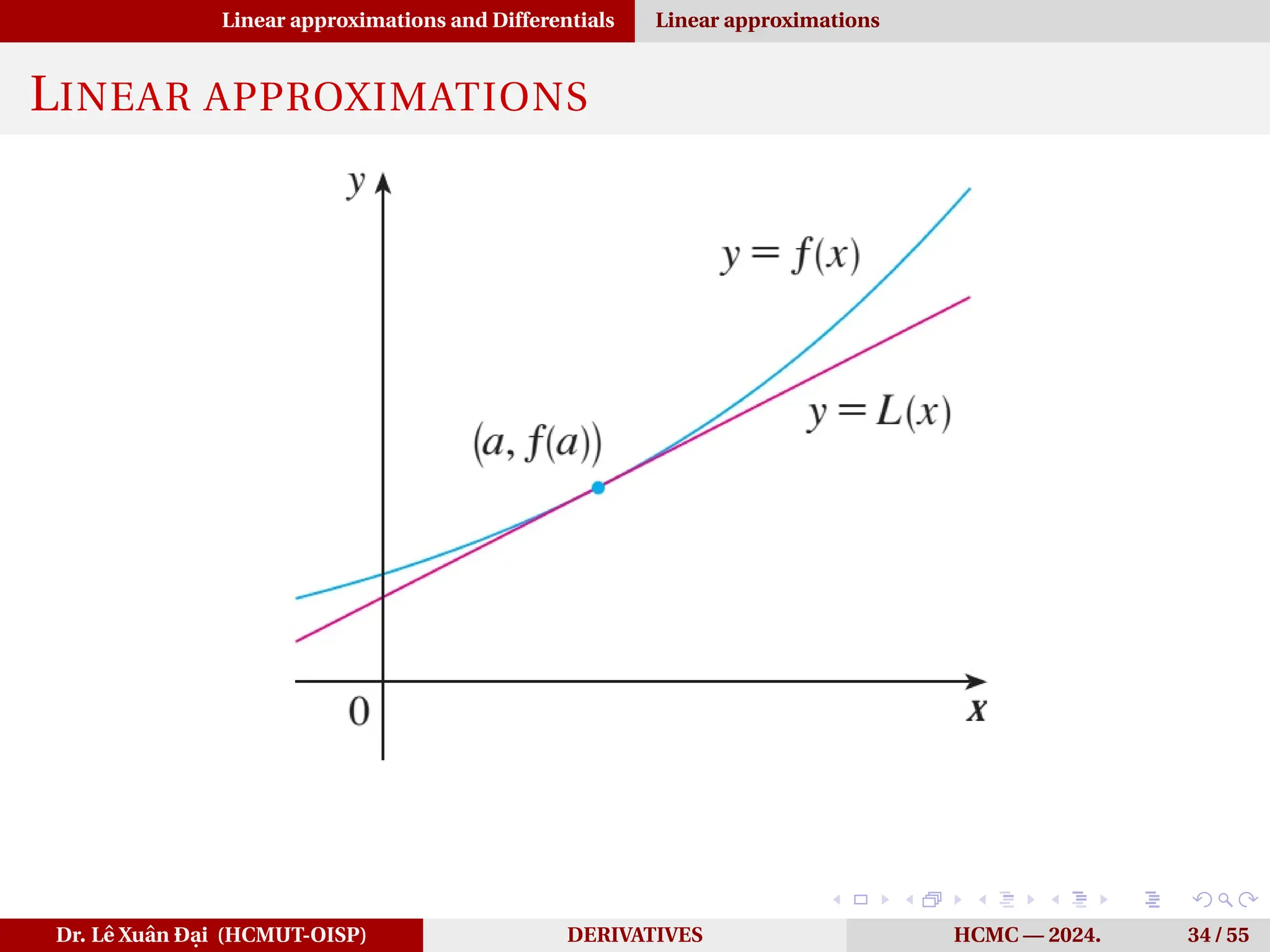
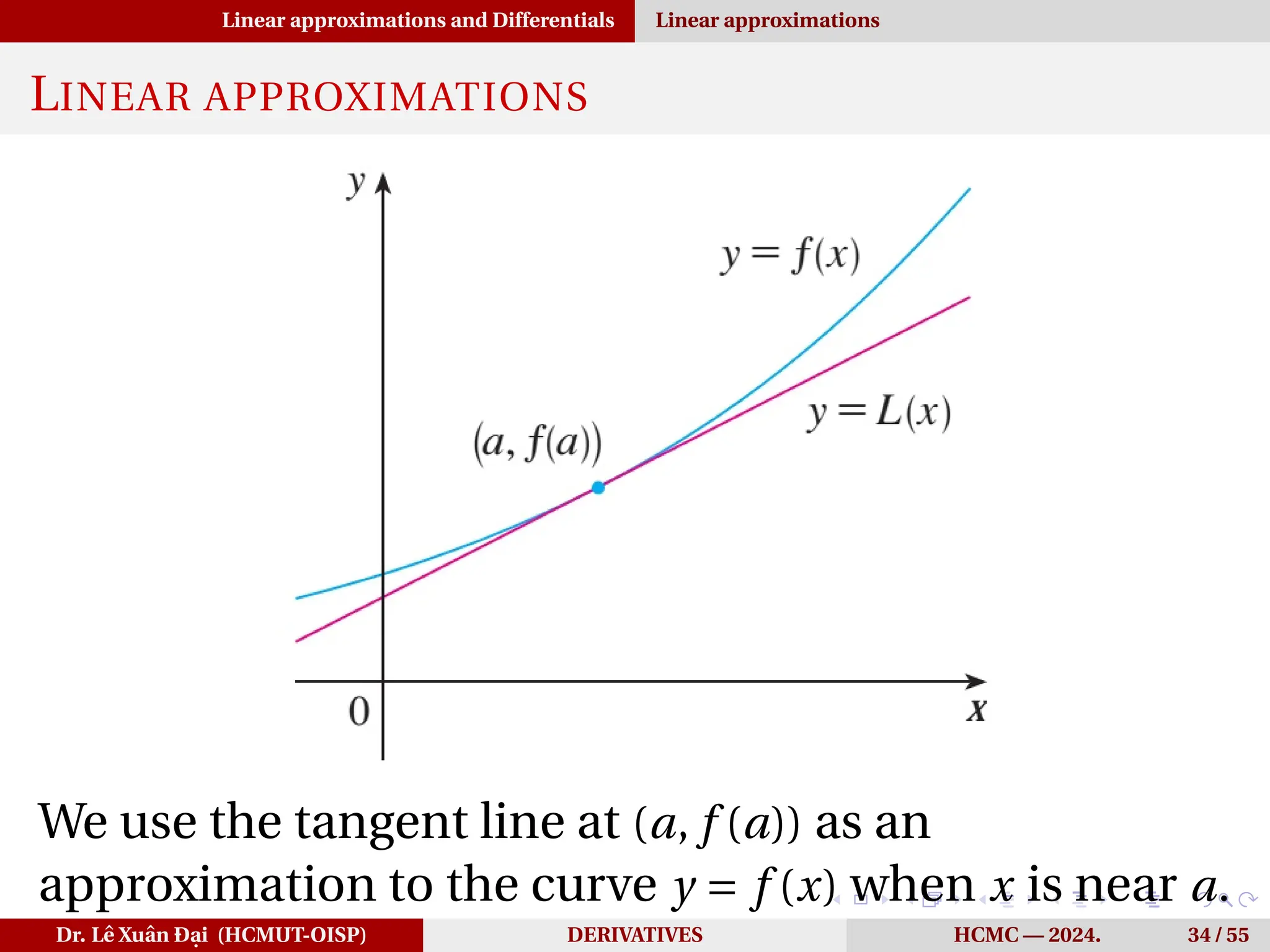
LINEAR APPROXIMATIONS
We use the tangent line at (a, f (a)) as an
approximation to the curve y = f (x) when x is near a.
Dr. Lê Xuân Đại (HCMUT-OISP) DERIVATIVES HCMC — 2024. 34 / 55
59.
Linear approximations andDifferentials Linear approximations
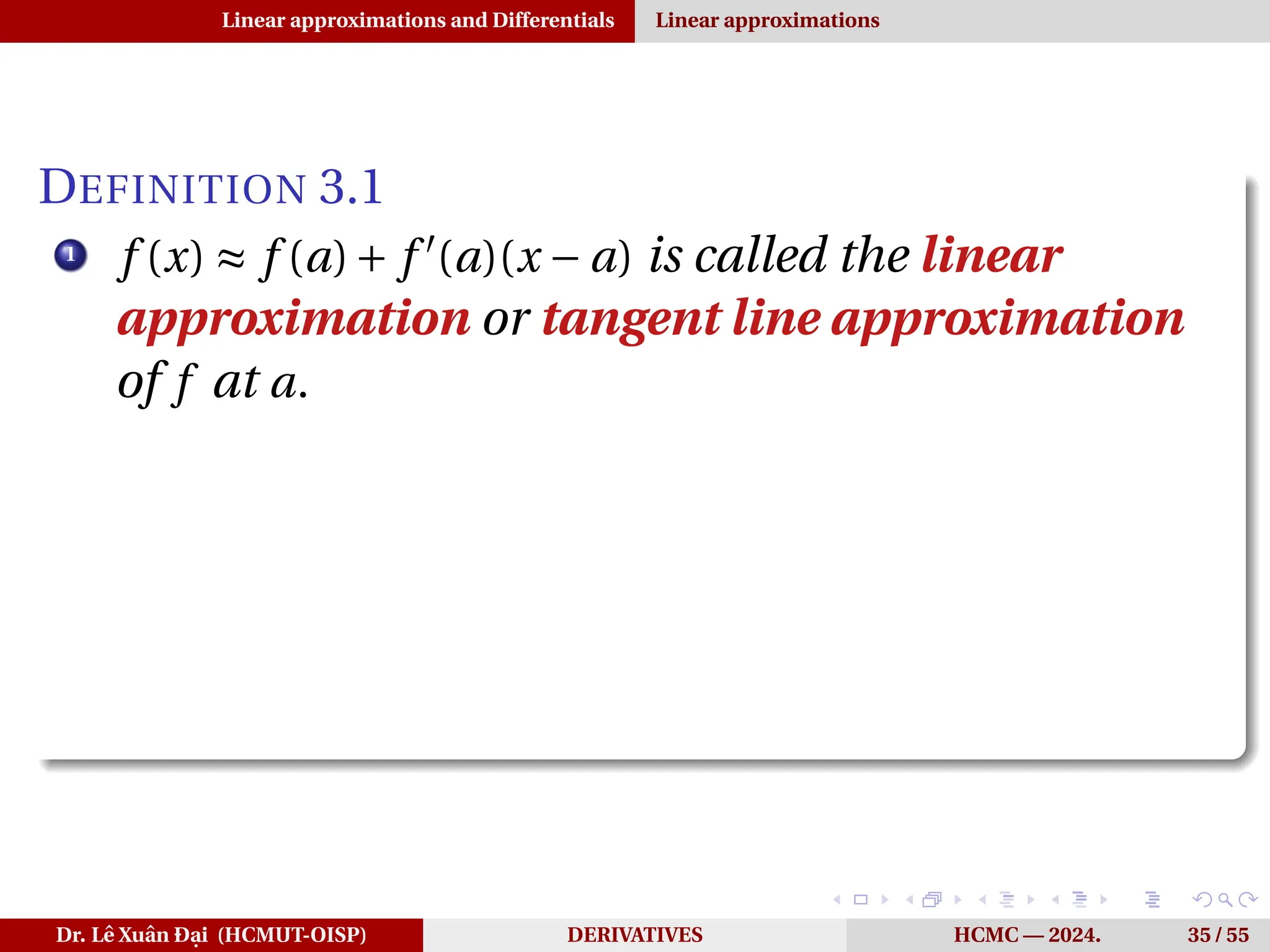
DEFINITION 3.1
1
f (x) ≈ f (a)+ f ′
(a)(x − a) is called the linear
approximation or tangent line approximation
of f at a.
Dr. Lê Xuân Đại (HCMUT-OISP) DERIVATIVES HCMC — 2024. 35 / 55
60.
Linear approximations andDifferentials Linear approximations
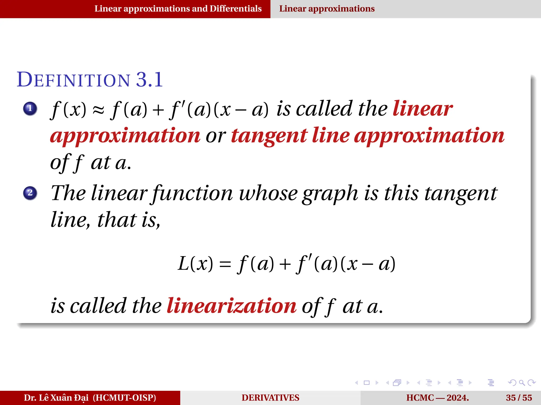
DEFINITION 3.1
1
f (x) ≈ f (a)+ f ′
(a)(x − a) is called the linear
approximation or tangent line approximation
of f at a.
2
The linear function whose graph is this tangent
line, that is,
L(x) = f (a)+ f ′
(a)(x − a)
is called the linearization of f at a.
Dr. Lê Xuân Đại (HCMUT-OISP) DERIVATIVES HCMC — 2024. 35 / 55
61.
Linear approximations andDifferentials Linear approximations
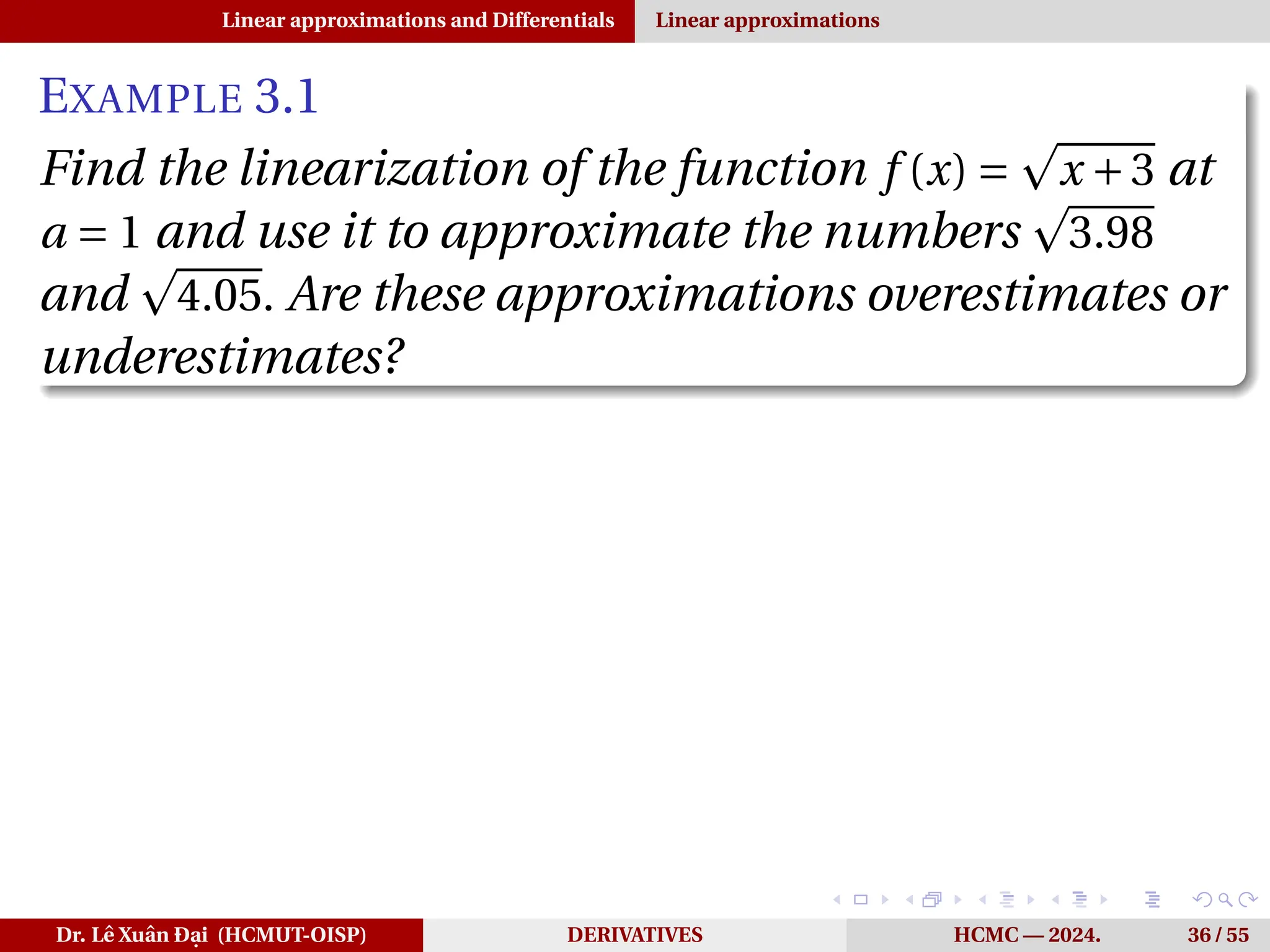
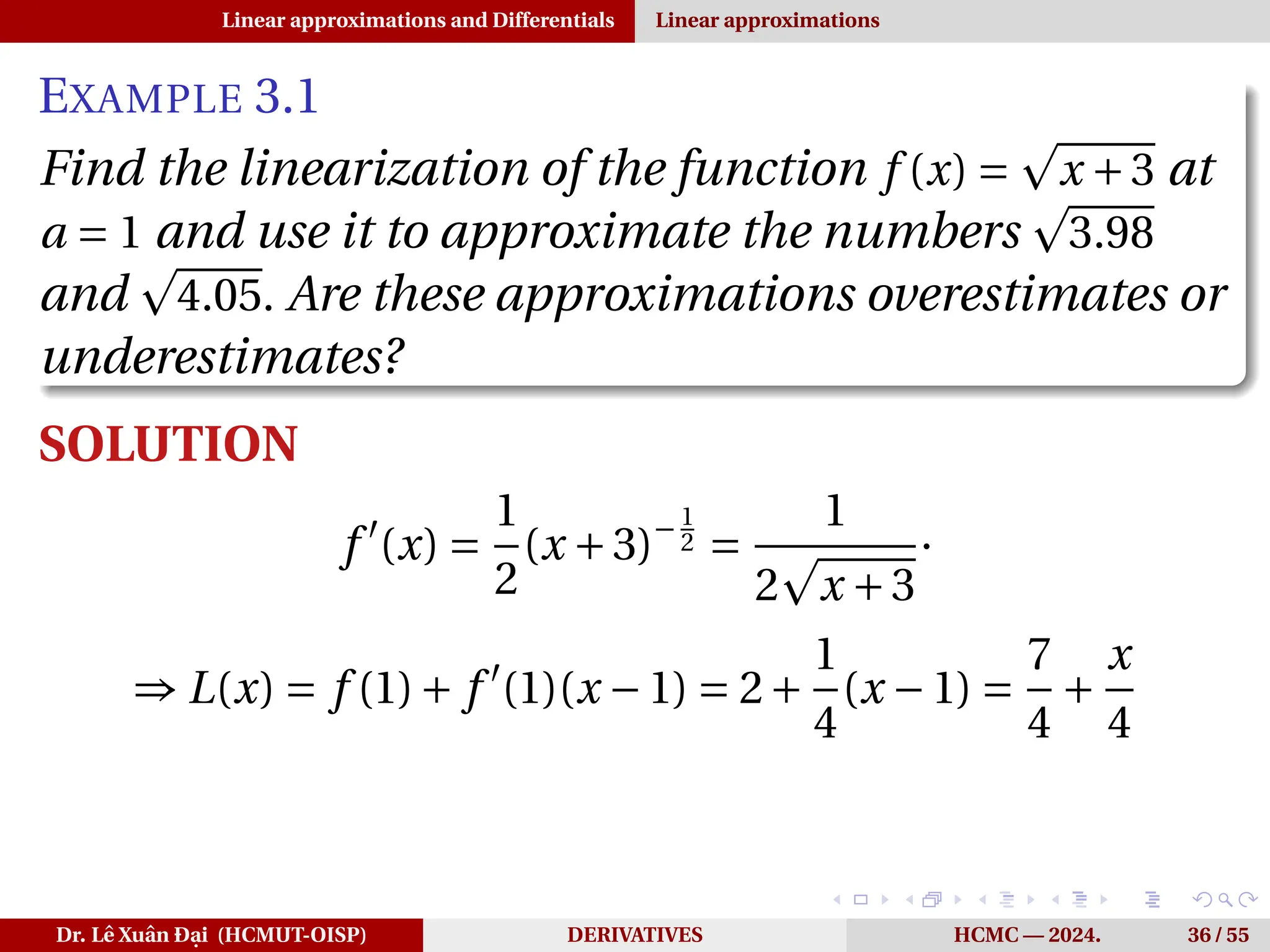
EXAMPLE 3.1
Find the linearization of the function f (x) =
p
x +3 at
a = 1 and use it to approximate the numbers
p
3.98
and
p
4.05. Are these approximations overestimates or
underestimates?
Dr. Lê Xuân Đại (HCMUT-OISP) DERIVATIVES HCMC — 2024. 36 / 55
62.
Linear approximations andDifferentials Linear approximations
EXAMPLE 3.1
Find the linearization of the function f (x) =
p
x +3 at
a = 1 and use it to approximate the numbers
p
3.98
and
p
4.05. Are these approximations overestimates or
underestimates?
SOLUTION
f ′
(x) =
1
2
(x +3)−1
2 =
1
2
p
x +3
·
⇒ L(x) = f (1)+ f ′
(1)(x −1) = 2+
1
4
(x −1) =
7
4
+
x
4
Dr. Lê Xuân Đại (HCMUT-OISP) DERIVATIVES HCMC — 2024. 36 / 55
63.
Linear approximations andDifferentials Linear approximations
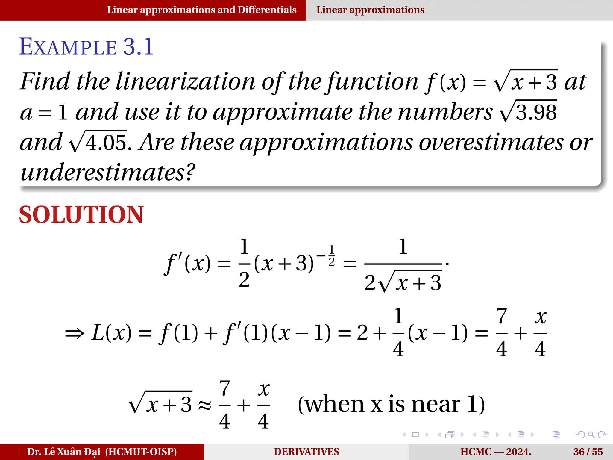
EXAMPLE 3.1
Find the linearization of the function f (x) =
p
x +3 at
a = 1 and use it to approximate the numbers
p
3.98
and
p
4.05. Are these approximations overestimates or
underestimates?
SOLUTION
f ′
(x) =
1
2
(x +3)−1
2 =
1
2
p
x +3
·
⇒ L(x) = f (1)+ f ′
(1)(x −1) = 2+
1
4
(x −1) =
7
4
+
x
4
p
x +3 ≈
7
4
+
x
4
(when x is near 1)
Dr. Lê Xuân Đại (HCMUT-OISP) DERIVATIVES HCMC — 2024. 36 / 55
64.
Linear approximations andDifferentials Linear approximations
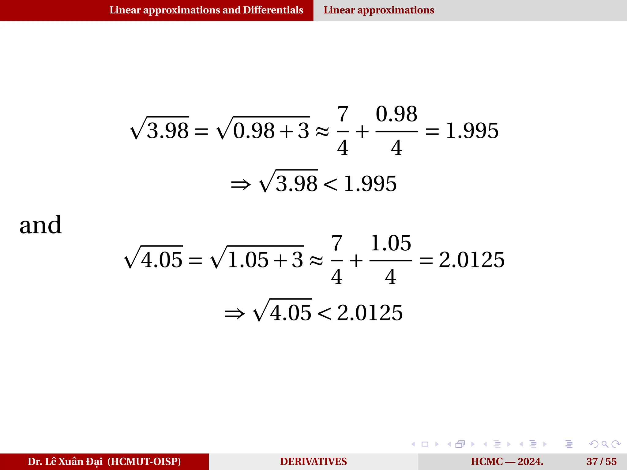
p
3.98 =
p
0.98+3 ≈
7
4
+
0.98
4
= 1.995
⇒
p
3.98 < 1.995
and
p
4.05 =
p
1.05+3 ≈
7
4
+
1.05
4
= 2.0125
⇒
p
4.05 < 2.0125
Dr. Lê Xuân Đại (HCMUT-OISP) DERIVATIVES HCMC — 2024. 37 / 55
65.
Linear approximations andDifferentials Linear approximations
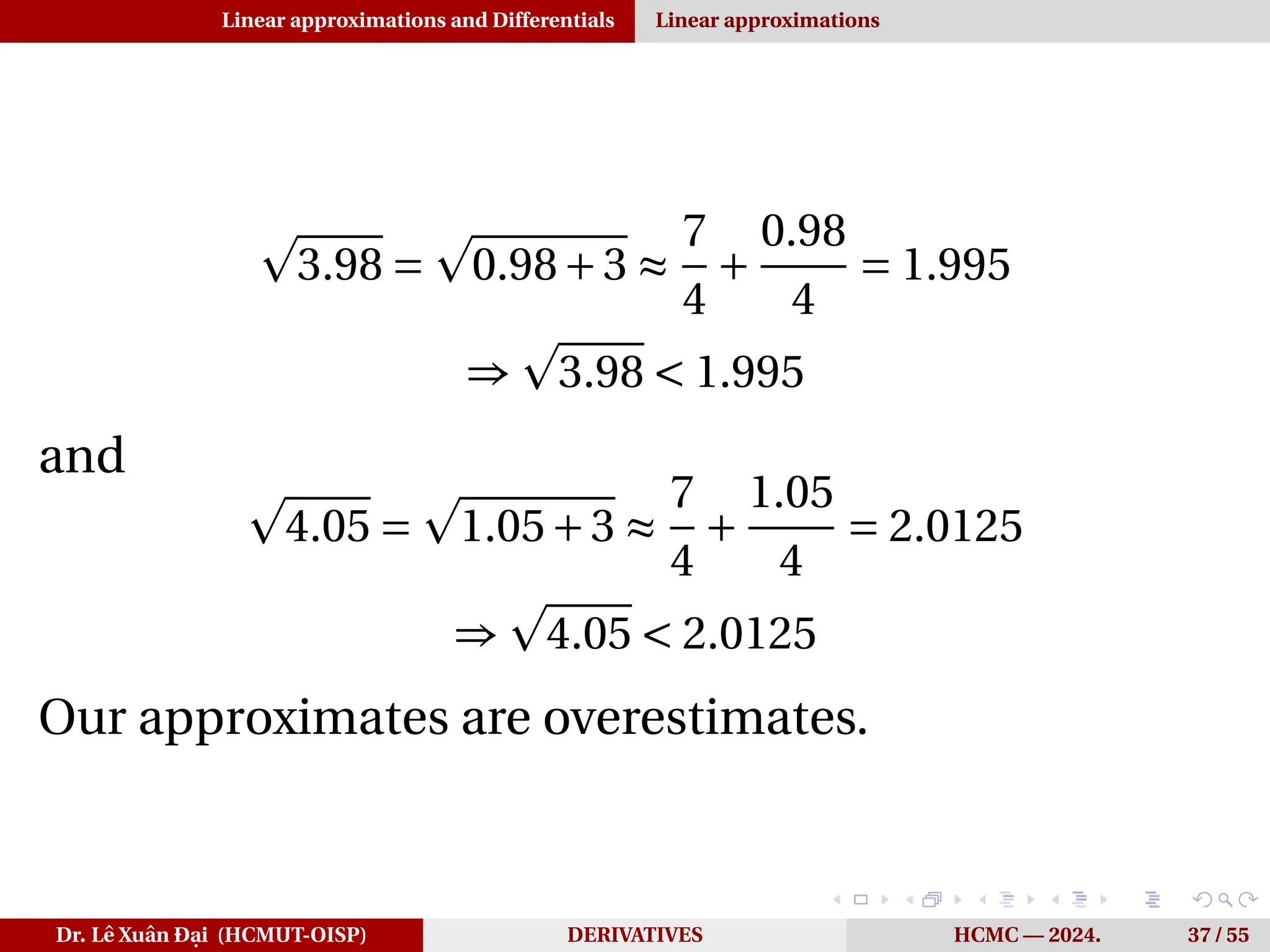
p
3.98 =
p
0.98+3 ≈
7
4
+
0.98
4
= 1.995
⇒
p
3.98 < 1.995
and
p
4.05 =
p
1.05+3 ≈
7
4
+
1.05
4
= 2.0125
⇒
p
4.05 < 2.0125
Our approximates are overestimates.
Dr. Lê Xuân Đại (HCMUT-OISP) DERIVATIVES HCMC — 2024. 37 / 55
66.
Linear approximations andDifferentials The 1-st order differentials
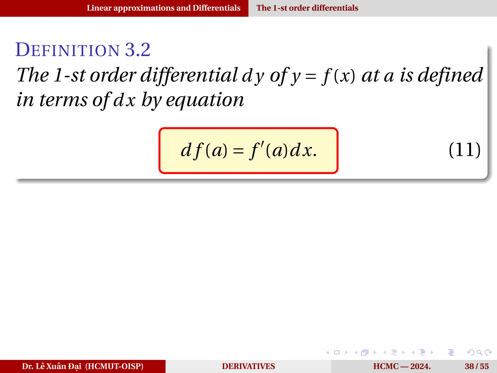
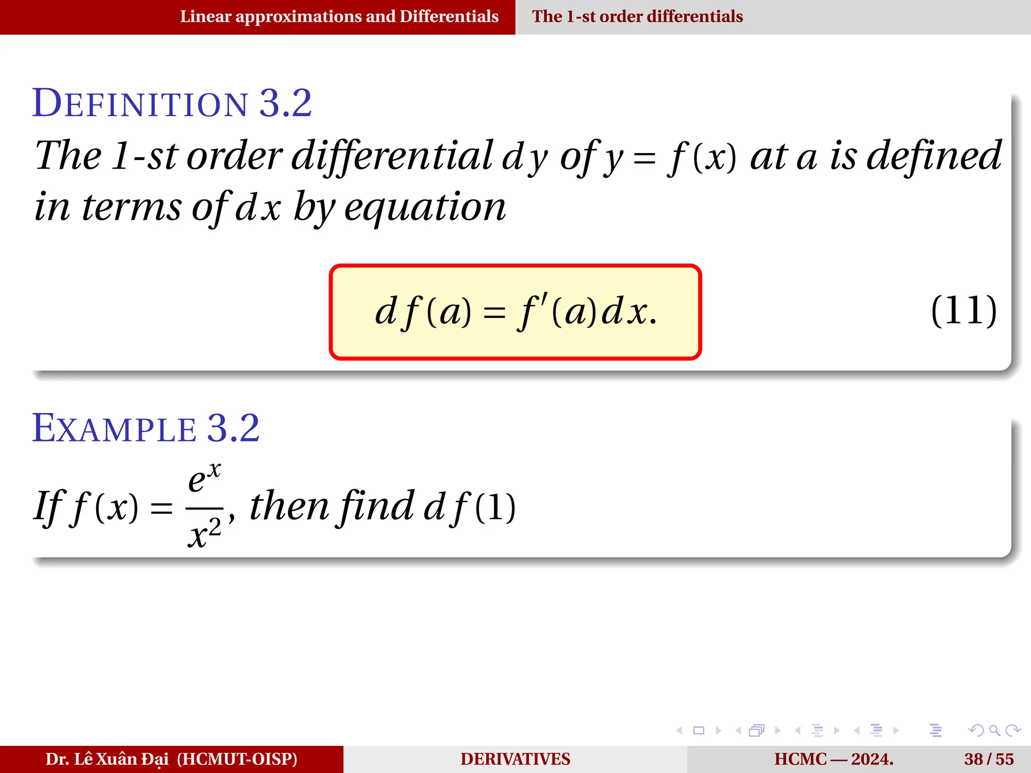
DEFINITION 3.2
The 1-st order differential d y of y = f (x) at a is defined
in terms of dx by equation
d f (a) = f ′
(a)dx. (11)
Dr. Lê Xuân Đại (HCMUT-OISP) DERIVATIVES HCMC — 2024. 38 / 55
67.
Linear approximations andDifferentials The 1-st order differentials
DEFINITION 3.2
The 1-st order differential d y of y = f (x) at a is defined
in terms of dx by equation
d f (a) = f ′
(a)dx. (11)
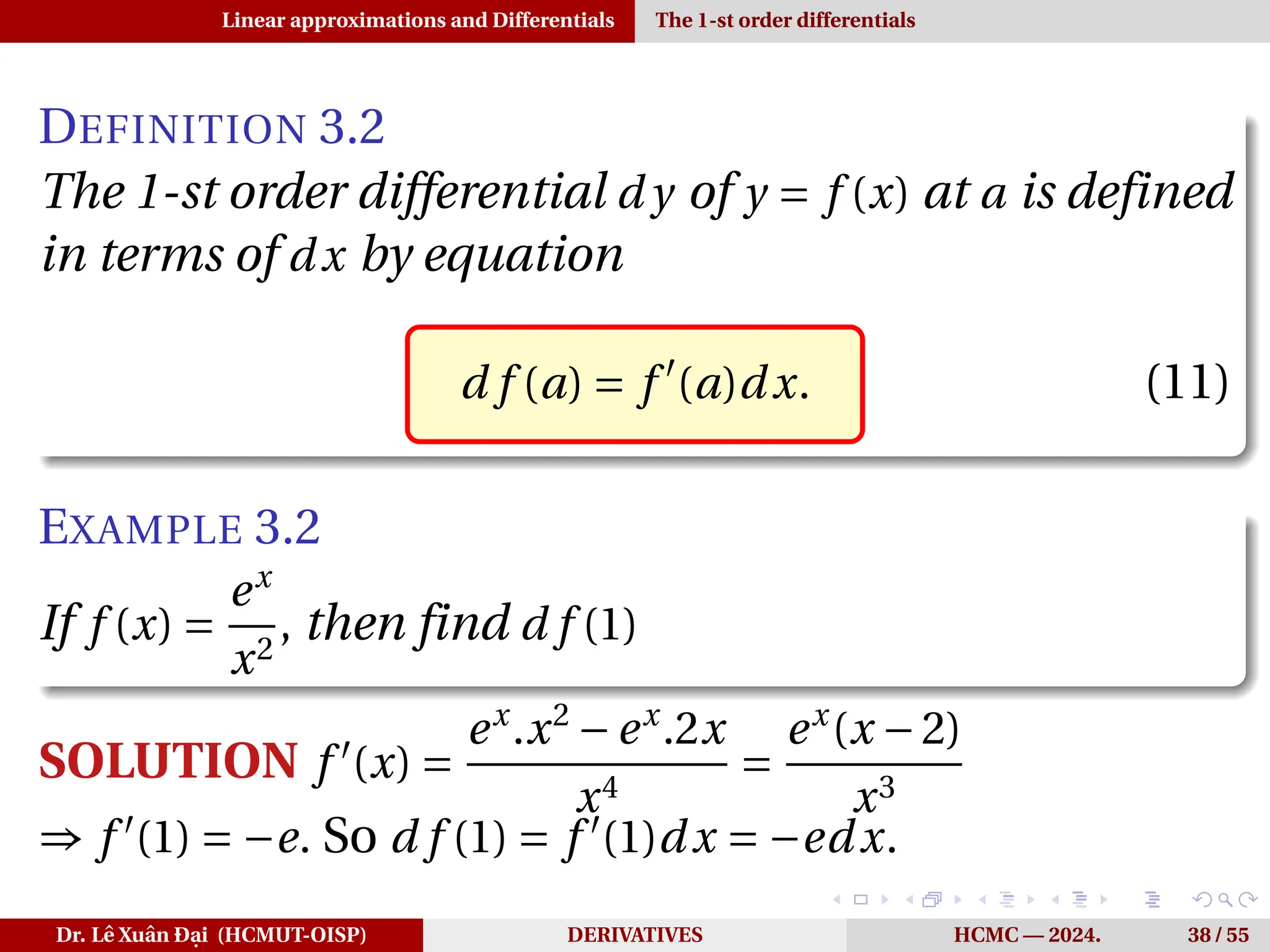
EXAMPLE 3.2
If f (x) =
ex
x2
, then find d f (1)
Dr. Lê Xuân Đại (HCMUT-OISP) DERIVATIVES HCMC — 2024. 38 / 55
68.
Linear approximations andDifferentials The 1-st order differentials
DEFINITION 3.2
The 1-st order differential d y of y = f (x) at a is defined
in terms of dx by equation
d f (a) = f ′
(a)dx. (11)
EXAMPLE 3.2
If f (x) =
ex
x2
, then find d f (1)
SOLUTION f ′
(x) =
ex
.x2
−ex
.2x
x4
=
ex
(x −2)
x3
⇒ f ′
(1) = −e. So d f (1) = f ′
(1)dx = −edx.
Dr. Lê Xuân Đại (HCMUT-OISP) DERIVATIVES HCMC — 2024. 38 / 55
69.
Linear approximations andDifferentials The 1-st order differentials
THE GEOMETRIC MEANING OF DIFFERENTIALS
Dr. Lê Xuân Đại (HCMUT-OISP) DERIVATIVES HCMC — 2024. 39 / 55
70.
Linear approximations andDifferentials The 1-st order differentials
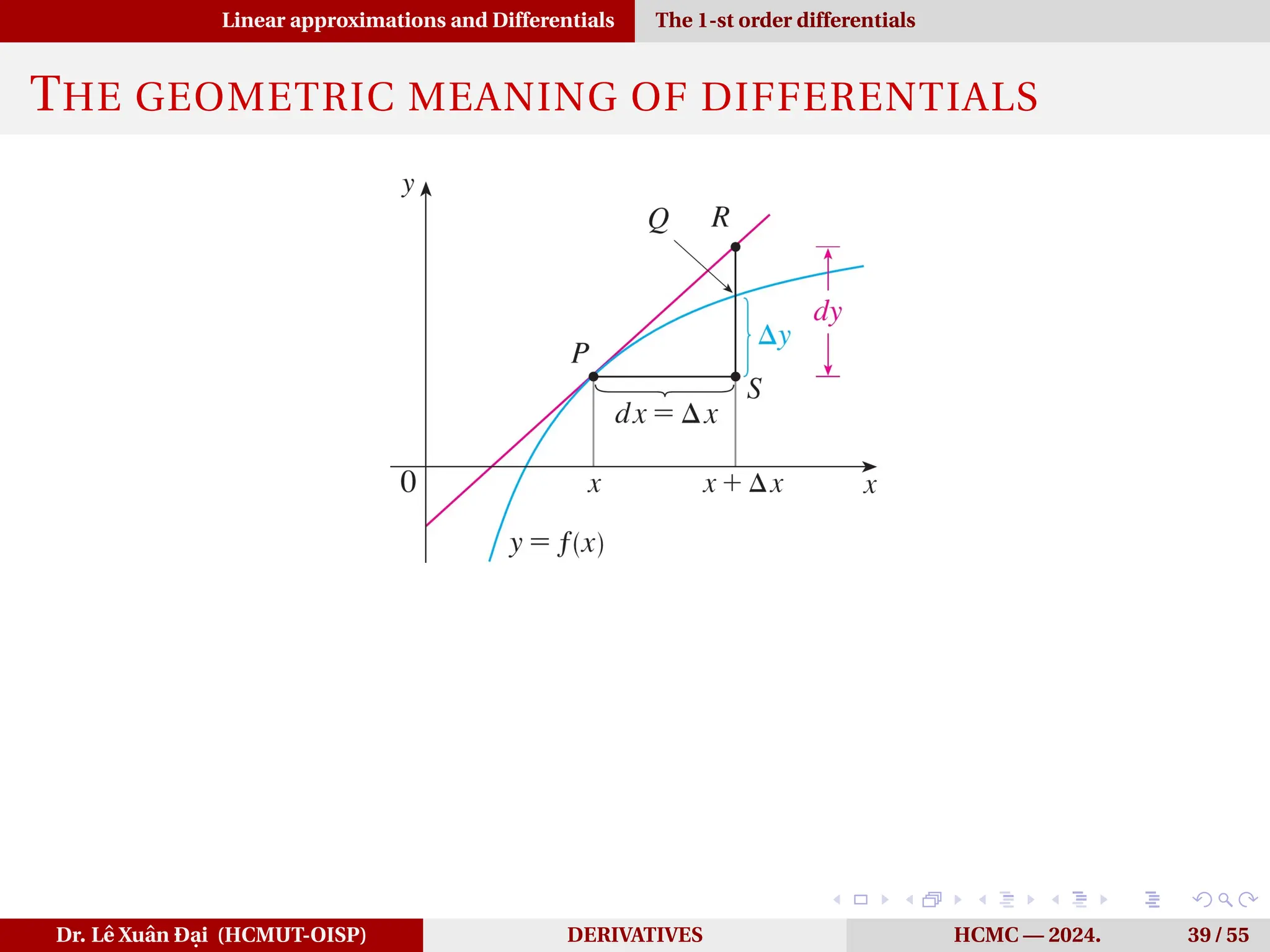
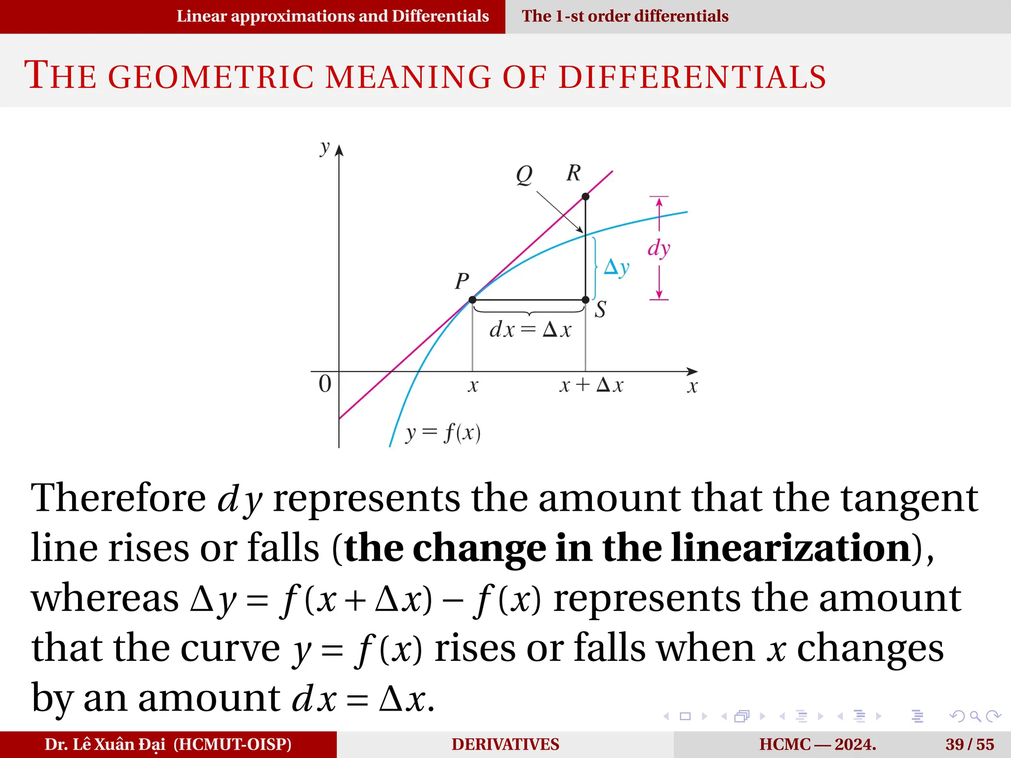
THE GEOMETRIC MEANING OF DIFFERENTIALS
Therefore d y represents the amount that the tangent
line rises or falls (the change in the linearization),
whereas ∆y = f (x +∆x)− f (x) represents the amount
that the curve y = f (x) rises or falls when x changes
by an amount dx = ∆x.
Dr. Lê Xuân Đại (HCMUT-OISP) DERIVATIVES HCMC — 2024. 39 / 55
71.
Linear approximations andDifferentials The 1-st order differentials
EXAMPLE 3.3
Compare the values of ∆y and d y if
y = f (x) = x3
+ x2
−2x +1 and x changes
1
from 2 to 2.05
Dr. Lê Xuân Đại (HCMUT-OISP) DERIVATIVES HCMC — 2024. 40 / 55
72.
Linear approximations andDifferentials The 1-st order differentials
EXAMPLE 3.3
Compare the values of ∆y and d y if
y = f (x) = x3
+ x2
−2x +1 and x changes
1
from 2 to 2.05 2
from 2 to 2.01
Dr. Lê Xuân Đại (HCMUT-OISP) DERIVATIVES HCMC — 2024. 40 / 55
73.
Linear approximations andDifferentials The 1-st order differentials
EXAMPLE 3.3
Compare the values of ∆y and d y if
y = f (x) = x3
+ x2
−2x +1 and x changes
1
from 2 to 2.05 2
from 2 to 2.01
SOLUTION d y = f ′
(x)dx = (3x2
+2x −2)dx.
1
f (2) = 9, f (2.05) = 9.717625 ⇒ ∆y = 0.717625. When
x = 2 and dx = ∆x = 2.05−2 = 0.05, this becomes
d y = [3(2)2
+2(2)−2]0.05 = 0.7
Dr. Lê Xuân Đại (HCMUT-OISP) DERIVATIVES HCMC — 2024. 40 / 55
74.
Linear approximations andDifferentials The 1-st order differentials
EXAMPLE 3.3
Compare the values of ∆y and d y if
y = f (x) = x3
+ x2
−2x +1 and x changes
1
from 2 to 2.05 2
from 2 to 2.01
SOLUTION d y = f ′
(x)dx = (3x2
+2x −2)dx.
1
f (2) = 9, f (2.05) = 9.717625 ⇒ ∆y = 0.717625. When
x = 2 and dx = ∆x = 2.05−2 = 0.05, this becomes
d y = [3(2)2
+2(2)−2]0.05 = 0.7
2
f (2) = 9, f (2.01) = 9.140701 ⇒ ∆y = 0.140701. When
x = 2 and dx = ∆x = 2.01−2 = 0.01, this becomes
d y = [3(2)2
+2(2)−2]0.01 = 0.14
Dr. Lê Xuân Đại (HCMUT-OISP) DERIVATIVES HCMC — 2024. 40 / 55
75.
Linear approximations andDifferentials The 1-st order differentials
EXAMPLE 3.3
Compare the values of ∆y and d y if
y = f (x) = x3
+ x2
−2x +1 and x changes
1
from 2 to 2.05 2
from 2 to 2.01
SOLUTION d y = f ′
(x)dx = (3x2
+2x −2)dx.
1
f (2) = 9, f (2.05) = 9.717625 ⇒ ∆y = 0.717625. When
x = 2 and dx = ∆x = 2.05−2 = 0.05, this becomes
d y = [3(2)2
+2(2)−2]0.05 = 0.7
2
f (2) = 9, f (2.01) = 9.140701 ⇒ ∆y = 0.140701. When
x = 2 and dx = ∆x = 2.01−2 = 0.01, this becomes
d y = [3(2)2
+2(2)−2]0.01 = 0.14
∆y ≈ d y becomes better as ∆x becomes smaller.
Dr. Lê Xuân Đại (HCMUT-OISP) DERIVATIVES HCMC — 2024. 40 / 55
76.
Linear approximations andDifferentials The 2-nd order differentials
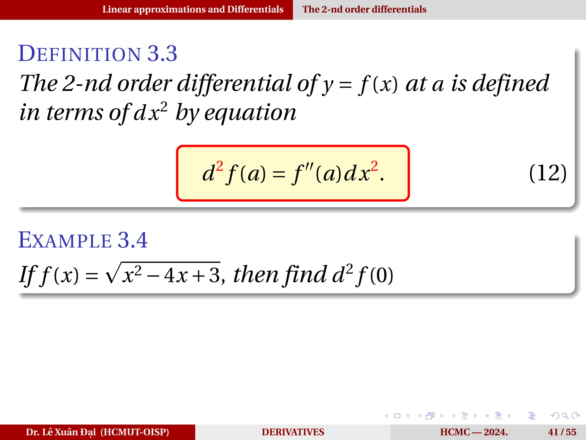
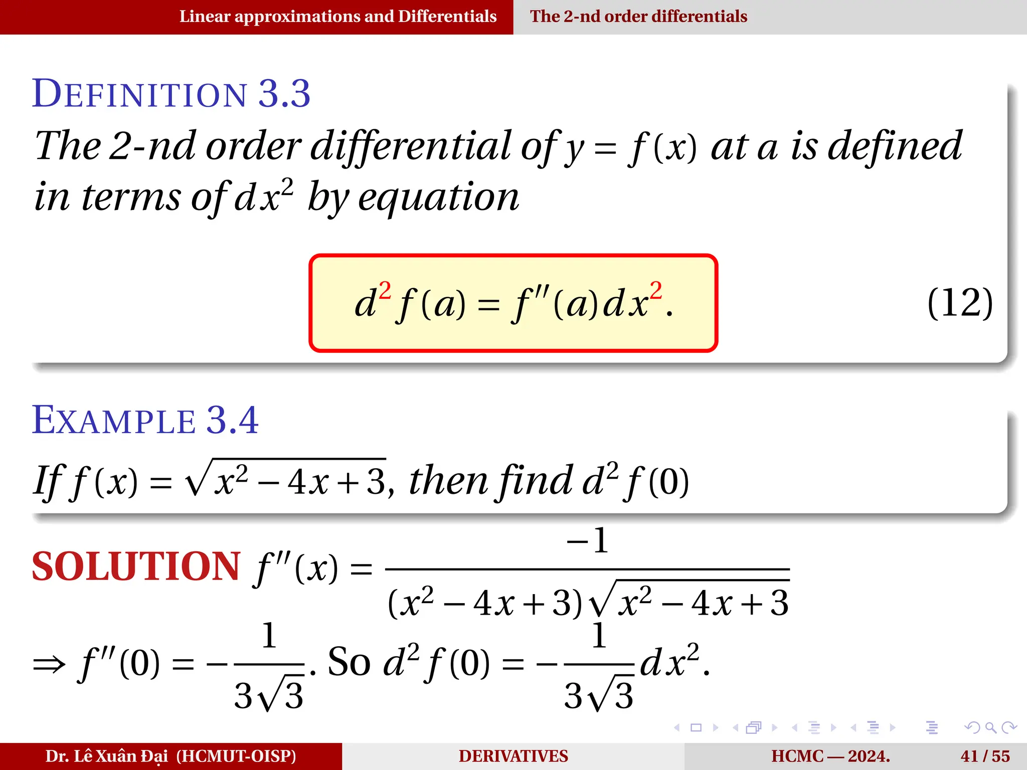
DEFINITION 3.3
The 2-nd order differential of y = f (x) at a is defined
in terms of dx2
by equation
d2
f (a) = f ′′
(a)dx2
. (12)
Dr. Lê Xuân Đại (HCMUT-OISP) DERIVATIVES HCMC — 2024. 41 / 55
77.
Linear approximations andDifferentials The 2-nd order differentials
DEFINITION 3.3
The 2-nd order differential of y = f (x) at a is defined
in terms of dx2
by equation
d2
f (a) = f ′′
(a)dx2
. (12)
EXAMPLE 3.4
If f (x) =
p
x2 −4x +3, then find d2
f (0)
Dr. Lê Xuân Đại (HCMUT-OISP) DERIVATIVES HCMC — 2024. 41 / 55
78.
Linear approximations andDifferentials The 2-nd order differentials
DEFINITION 3.3
The 2-nd order differential of y = f (x) at a is defined
in terms of dx2
by equation
d2
f (a) = f ′′
(a)dx2
. (12)
EXAMPLE 3.4
If f (x) =
p
x2 −4x +3, then find d2
f (0)
SOLUTION f ′′
(x) =
−1
(x2 −4x +3)
p
x2 −4x +3
⇒ f ′′
(0) = −
1
3
p
3
. So d2
f (0) = −
1
3
p
3
dx2
.
Dr. Lê Xuân Đại (HCMUT-OISP) DERIVATIVES HCMC — 2024. 41 / 55
79.
Linear approximations andDifferentials The n−th order differentials
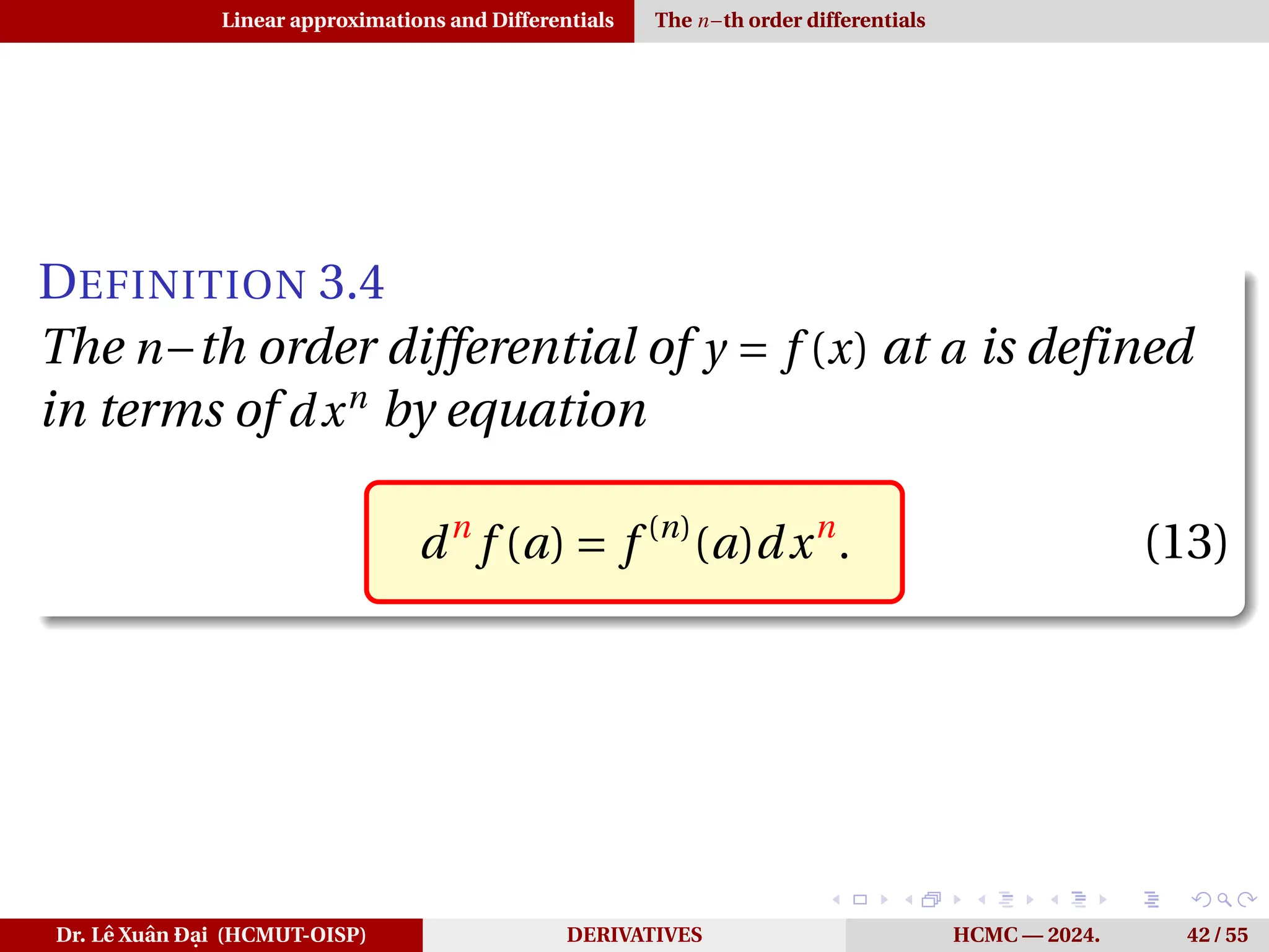
DEFINITION 3.4
The n−th order differential of y = f (x) at a is defined
in terms of dxn
by equation
dn
f (a) = f (n)
(a)dxn
. (13)
Dr. Lê Xuân Đại (HCMUT-OISP) DERIVATIVES HCMC — 2024. 42 / 55
80.
Rates of changeand Related rates Rates of change in the natural and social sciences
RATES OF CHANGE
Dr. Lê Xuân Đại (HCMUT-OISP) DERIVATIVES HCMC — 2024. 43 / 55
81.
Rates of changeand Related rates Rates of change in the natural and social sciences
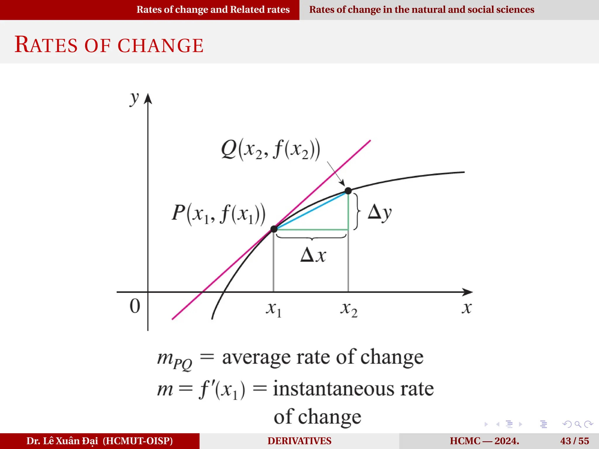
RATES OF CHANGE
If x changes from x1 to x2, then the change in x is
∆x = x2 − x1 and the corresponding change in y is
∆y = f (x2)− f (x1). The difference quotient
∆y
∆x
=
f (x2)− f (x1)
x2 − x1
is the average rate of change of y with respect to x
over the interval [x1,x2].
Dr. Lê Xuân Đại (HCMUT-OISP) DERIVATIVES HCMC — 2024. 44 / 55
82.
Rates of changeand Related rates Rates of change in the natural and social sciences
RATES OF CHANGE
If x changes from x1 to x2, then the change in x is
∆x = x2 − x1 and the corresponding change in y is
∆y = f (x2)− f (x1). The difference quotient
∆y
∆x
=
f (x2)− f (x1)
x2 − x1
is the average rate of change of y with respect to x
over the interval [x1,x2].
The instantaneous rate of change of y with respect to
x or the slope of the tangent line at P(x1, f (x1)) is
d y
dx
= lim
∆x→0
∆y
∆x
Dr. Lê Xuân Đại (HCMUT-OISP) DERIVATIVES HCMC — 2024. 44 / 55
83.
Rates of changeand Related rates Rates of change in the natural and social sciences
PHYSICS
If s = f (t) is the position function of a particle that is
moving in a straight line, then
1
∆s
∆t
represents the average velocity over a time
period ∆t
Dr. Lê Xuân Đại (HCMUT-OISP) DERIVATIVES HCMC — 2024. 45 / 55
84.
Rates of changeand Related rates Rates of change in the natural and social sciences
PHYSICS
If s = f (t) is the position function of a particle that is
moving in a straight line, then
1
∆s
∆t
represents the average velocity over a time
period ∆t
2
ds
dt
= lim
∆t→0
∆s
∆t
represents the instantaneous
velocity
Dr. Lê Xuân Đại (HCMUT-OISP) DERIVATIVES HCMC — 2024. 45 / 55
85.
Rates of changeand Related rates Rates of change in the natural and social sciences
PHYSICS
If s = f (t) is the position function of a particle that is
moving in a straight line, then
1
∆s
∆t
represents the average velocity over a time
period ∆t
2
ds
dt
= lim
∆t→0
∆s
∆t
represents the instantaneous
velocity
3
the instantaneous rate of change of velocity with
respect to time is acceleration: a(t) = v′
(t) = s′′
(t).
Dr. Lê Xuân Đại (HCMUT-OISP) DERIVATIVES HCMC — 2024. 45 / 55
86.
Rates of changeand Related rates Rates of change in the natural and social sciences
EXAMPLE 4.1
The position of a particle is given by the equation
s = f (t) = t3
−6t2
+9t,
where t is measured in seconds and s in meters.
1
Find the velocity at time t.
Dr. Lê Xuân Đại (HCMUT-OISP) DERIVATIVES HCMC — 2024. 46 / 55
87.
Rates of changeand Related rates Rates of change in the natural and social sciences
EXAMPLE 4.1
The position of a particle is given by the equation
s = f (t) = t3
−6t2
+9t,
where t is measured in seconds and s in meters.
1
Find the velocity at time t. What is the velocity
after 2s?
Dr. Lê Xuân Đại (HCMUT-OISP) DERIVATIVES HCMC — 2024. 46 / 55
88.
Rates of changeand Related rates Rates of change in the natural and social sciences
EXAMPLE 4.1
The position of a particle is given by the equation
s = f (t) = t3
−6t2
+9t,
where t is measured in seconds and s in meters.
1
Find the velocity at time t. What is the velocity
after 2s? When is the particle at rest?
Dr. Lê Xuân Đại (HCMUT-OISP) DERIVATIVES HCMC — 2024. 46 / 55
89.
Rates of changeand Related rates Rates of change in the natural and social sciences
EXAMPLE 4.1
The position of a particle is given by the equation
s = f (t) = t3
−6t2
+9t,
where t is measured in seconds and s in meters.
1
Find the velocity at time t. What is the velocity
after 2s? When is the particle at rest? When is the
particle moving forward (that is, in the positive
direction) and backward?
2
Find the total distance travelled by the particle
during the first five seconds.
Dr. Lê Xuân Đại (HCMUT-OISP) DERIVATIVES HCMC — 2024. 46 / 55
90.
Rates of changeand Related rates Rates of change in the natural and social sciences
EXAMPLE 4.1
The position of a particle is given by the equation
s = f (t) = t3
−6t2
+9t,
where t is measured in seconds and s in meters.
1
Find the velocity at time t. What is the velocity
after 2s? When is the particle at rest? When is the
particle moving forward (that is, in the positive
direction) and backward?
2
Find the total distance travelled by the particle
during the first five seconds.
3
Find the acceleration at time t and after 4s.
Dr. Lê Xuân Đại (HCMUT-OISP) DERIVATIVES HCMC — 2024. 46 / 55
91.
Rates of changeand Related rates Rates of change in the natural and social sciences
EXAMPLE 4.1
The position of a particle is given by the equation
s = f (t) = t3
−6t2
+9t,
where t is measured in seconds and s in meters.
1
Find the velocity at time t. What is the velocity
after 2s? When is the particle at rest? When is the
particle moving forward (that is, in the positive
direction) and backward?
2
Find the total distance travelled by the particle
during the first five seconds.
3
Find the acceleration at time t and after 4s. When
is the particle speeding up,
Dr. Lê Xuân Đại (HCMUT-OISP) DERIVATIVES HCMC — 2024. 46 / 55
92.
Rates of changeand Related rates Rates of change in the natural and social sciences
EXAMPLE 4.1
The position of a particle is given by the equation
s = f (t) = t3
−6t2
+9t,
where t is measured in seconds and s in meters.
1
Find the velocity at time t. What is the velocity
after 2s? When is the particle at rest? When is the
particle moving forward (that is, in the positive
direction) and backward?
2
Find the total distance travelled by the particle
during the first five seconds.
3
Find the acceleration at time t and after 4s. When
is the particle speeding up, slowing down?
Dr. Lê Xuân Đại (HCMUT-OISP) DERIVATIVES HCMC — 2024. 46 / 55
93.
Rates of changeand Related rates Rates of change in the natural and social sciences
1
The velocity function
v(t) = s′
(t) = 3t2
−12t +9 ⇒ v(2) = −3m/s.
The particle is at rest when
v(t) = 0 ⇔ 3t2
−12t +9 = 0 ⇔
·
t = 1s
t = 3s.
The particle
moves forward when
v(t) > 0 ⇔
·
t > 3
t < 1
It moves backward then 1 < t < 3.
Dr. Lê Xuân Đại (HCMUT-OISP) DERIVATIVES HCMC — 2024. 47 / 55
94.
Rates of changeand Related rates Rates of change in the natural and social sciences
2
We need to calculate the distances travelled by
the particle during the time intervals [0,1],[1,3]
and [3,5] separately.
|f (1)− f (0)|+|f (3)− f (1)|+|f (5)− f (3)| =
= |4−0|+|0−4|+|20−0| = 4+4+20 = 28m.
Dr. Lê Xuân Đại (HCMUT-OISP) DERIVATIVES HCMC — 2024. 48 / 55
95.
Rates of changeand Related rates Rates of change in the natural and social sciences
3
The acceleration is the derivative of the velocity
function:
a(t) = v′
(t) = s′′
(t) = 6t −12 ⇒ a(4) = 12m/s2
4
The particle speeds up when the velocity is
positive and increasing (it means v(t) and a(t) are
both positive) and also when the velocity is
negative and decreasing (it means v(t) and a(t)
are both negative). In other words, the particle
speeds up when the velocity and acceleration
have the same sign.
v(t).a(t) > 0 ⇔ (3t2
−12t +9)(6t −12) > 0
Dr. Lê Xuân Đại (HCMUT-OISP) DERIVATIVES HCMC — 2024. 49 / 55
96.
Rates of changeand Related rates Rates of change in the natural and social sciences
= 18(t −1)(t −3)(t −2) > 0 ⇔
·
t > 3
1 < t < 2
5
The particle slows down when v(t) and a(t) have
opposite signs v(t).a(t) < 0 ⇔
·
2 < t < 3
0 < t < 1
Dr. Lê Xuân Đại (HCMUT-OISP) DERIVATIVES HCMC — 2024. 50 / 55
97.
Rates of changeand Related rates Related rates
RELATED RATES
* If we are pumping air into a balloon, both
the volume and the radius of the balloon
are increasing and their rates of increase
are related to each other.
Dr. Lê Xuân Đại (HCMUT-OISP) DERIVATIVES HCMC — 2024. 51 / 55
98.
Rates of changeand Related rates Related rates
RELATED RATES
* If we are pumping air into a balloon, both
the volume and the radius of the balloon
are increasing and their rates of increase
are related to each other.
* In a related rates problem the idea is to
compute the rate of change of one quantity
in terms of the rate of change of another
quatity.
Dr. Lê Xuân Đại (HCMUT-OISP) DERIVATIVES HCMC — 2024. 51 / 55
99.
Rates of changeand Related rates Related rates
RELATED RATES
* If we are pumping air into a balloon, both
the volume and the radius of the balloon
are increasing and their rates of increase
are related to each other.
* In a related rates problem the idea is to
compute the rate of change of one quantity
in terms of the rate of change of another
quatity.
* The procedure is to find an equation that
relates the two quantities and then use the
Chain Rule to differentiate both sides with
respect to time.
Dr. Lê Xuân Đại (HCMUT-OISP) DERIVATIVES HCMC — 2024. 51 / 55
100.
Rates of changeand Related rates Related rates
EXAMPLE 4.2
Air is being pumped into a spherical balloon so that
its volume increases at a rate of 100cm3
/s. How fast is
the radius of the balloon increasing when the
diameter is 50cm
SOLUTION Let V (t) be the volume of the balloon
and let r(t) be its radius. We start by identifying two
things
1
the given information: the rate of increase of the
volume of air is 100cm3
/s ⇒
dV
dt
= 100cm3
/s
Dr. Lê Xuân Đại (HCMUT-OISP) DERIVATIVES HCMC — 2024. 52 / 55
101.
Rates of changeand Related rates Related rates
2
the unknown: the rate of increase of the radius
when the diameter is 50cm ⇒
dr
dt
=? when
r = 25cm.
3
Equation that relates V (t) and r(t) is V =
4
3
πr3
4
Use the Chain Rule to differentiate both sides
with respect to time
dV
dt
=
dV
dr
·
dr
dt
= 4πr2
·
dr
dt
⇒
dr
dt
=
1
4πr2
·
dV
dt
Dr. Lê Xuân Đại (HCMUT-OISP) DERIVATIVES HCMC — 2024. 53 / 55
102.
Rates of changeand Related rates Related rates
If we put r = 25 and
dV
dt
= 100 in this equation, we
obtain
dr
dt
=
1
4π(25)2
·100 =
1
25π
≈ 0.0127cm/s.
Dr. Lê Xuân Đại (HCMUT-OISP) DERIVATIVES HCMC — 2024. 54 / 55
103.
Rates of changeand Related rates Related rates
THANK YOU FOR YOUR ATTENTION
Dr. Lê Xuân Đại (HCMUT-OISP) DERIVATIVES HCMC — 2024. 55 / 55
![Derivatives Velocities
Now suppose we compute the average velocities
over shorter and shorter time intervals [a,a +h]. We
let h approach 0. The instantaneous velocity v(a) at
time t = a is defined by
v(a) = lim
h→0
f (a +h)− f (a)
h
(2)
Dr. Lê Xuân Đại (HCMUT-OISP) DERIVATIVES HCMC — 2024. 7 / 55](https://image.slidesharecdn.com/derivatives-250903135428-da91ce23/75/derivativesderivativesderivativesderivatives-pdf-12-2048.jpg)
![Derivatives Definition
EXAMPLE 1.3
Find the derivative of the function f (x) = x2
−8x +9 at
the number a
SOLUTION
f ′
(a) = lim
h→0
f (a +h)− f (a)
h
=
= lim
h→0
[(a +h)2
−8(a +h)+9]−(a2
−8a +9)
h
=
= lim
h→0
a2
+2ah +h2
−8a −8h +9− a2
+8a −9
h
=
= lim
h→0
2ah +h2
−8h
h
= lim
h→0
(2a +h −8) = 2a −8
Dr. Lê Xuân Đại (HCMUT-OISP) DERIVATIVES HCMC — 2024. 11 / 55](https://image.slidesharecdn.com/derivatives-250903135428-da91ce23/75/derivativesderivativesderivativesderivatives-pdf-23-2048.jpg)
![Derivatives Definition
THEOREM 1.1
A function y = f (x) is differentiable at a if and only if
the left-hand and the right-hand derivatives of f at a
exist and are equal.
f ′
(a) = f ′
−(a) = f ′
+(a) (6)
DEFINITION 1.4
A function y = f (x) is differentiable on an open
interval (a,b) [or (a,∞) or (−∞,a) or (−∞,∞)] if it is
differentiable at every number in the interval.
Dr. Lê Xuân Đại (HCMUT-OISP) DERIVATIVES HCMC — 2024. 13 / 55](https://image.slidesharecdn.com/derivatives-250903135428-da91ce23/75/derivativesderivativesderivativesderivatives-pdf-27-2048.jpg)
![Derivatives The chain rule
EXAMPLE 1.5
Differentiate y = sin5
(4x +3)
SOLUTION
y′
= 5sin4
(4x +3).[sin(4x +3)]′
=
= 5sin4
(4x +3).cos(4x +3).(4x +3)′
=
= 20sin4
(4x +3)cos(4x +3).
Dr. Lê Xuân Đại (HCMUT-OISP) DERIVATIVES HCMC — 2024. 24 / 55](https://image.slidesharecdn.com/derivatives-250903135428-da91ce23/75/derivativesderivativesderivativesderivatives-pdf-42-2048.jpg)

![Linear approximations and Differentials The 1-st order differentials
EXAMPLE 3.3
Compare the values of ∆y and d y if
y = f (x) = x3
+ x2
−2x +1 and x changes
1
from 2 to 2.05 2
from 2 to 2.01
SOLUTION d y = f ′
(x)dx = (3x2
+2x −2)dx.
1
f (2) = 9, f (2.05) = 9.717625 ⇒ ∆y = 0.717625. When
x = 2 and dx = ∆x = 2.05−2 = 0.05, this becomes
d y = [3(2)2
+2(2)−2]0.05 = 0.7
Dr. Lê Xuân Đại (HCMUT-OISP) DERIVATIVES HCMC — 2024. 40 / 55](https://image.slidesharecdn.com/derivatives-250903135428-da91ce23/75/derivativesderivativesderivativesderivatives-pdf-73-2048.jpg)
![Linear approximations and Differentials The 1-st order differentials
EXAMPLE 3.3
Compare the values of ∆y and d y if
y = f (x) = x3
+ x2
−2x +1 and x changes
1
from 2 to 2.05 2
from 2 to 2.01
SOLUTION d y = f ′
(x)dx = (3x2
+2x −2)dx.
1
f (2) = 9, f (2.05) = 9.717625 ⇒ ∆y = 0.717625. When
x = 2 and dx = ∆x = 2.05−2 = 0.05, this becomes
d y = [3(2)2
+2(2)−2]0.05 = 0.7
2
f (2) = 9, f (2.01) = 9.140701 ⇒ ∆y = 0.140701. When
x = 2 and dx = ∆x = 2.01−2 = 0.01, this becomes
d y = [3(2)2
+2(2)−2]0.01 = 0.14
Dr. Lê Xuân Đại (HCMUT-OISP) DERIVATIVES HCMC — 2024. 40 / 55](https://image.slidesharecdn.com/derivatives-250903135428-da91ce23/75/derivativesderivativesderivativesderivatives-pdf-74-2048.jpg)
![Linear approximations and Differentials The 1-st order differentials
EXAMPLE 3.3
Compare the values of ∆y and d y if
y = f (x) = x3
+ x2
−2x +1 and x changes
1
from 2 to 2.05 2
from 2 to 2.01
SOLUTION d y = f ′
(x)dx = (3x2
+2x −2)dx.
1
f (2) = 9, f (2.05) = 9.717625 ⇒ ∆y = 0.717625. When
x = 2 and dx = ∆x = 2.05−2 = 0.05, this becomes
d y = [3(2)2
+2(2)−2]0.05 = 0.7
2
f (2) = 9, f (2.01) = 9.140701 ⇒ ∆y = 0.140701. When
x = 2 and dx = ∆x = 2.01−2 = 0.01, this becomes
d y = [3(2)2
+2(2)−2]0.01 = 0.14
∆y ≈ d y becomes better as ∆x becomes smaller.
Dr. Lê Xuân Đại (HCMUT-OISP) DERIVATIVES HCMC — 2024. 40 / 55](https://image.slidesharecdn.com/derivatives-250903135428-da91ce23/75/derivativesderivativesderivativesderivatives-pdf-75-2048.jpg)
![Rates of change and Related rates Rates of change in the natural and social sciences
RATES OF CHANGE
If x changes from x1 to x2, then the change in x is
∆x = x2 − x1 and the corresponding change in y is
∆y = f (x2)− f (x1). The difference quotient
∆y
∆x
=
f (x2)− f (x1)
x2 − x1
is the average rate of change of y with respect to x
over the interval [x1,x2].
Dr. Lê Xuân Đại (HCMUT-OISP) DERIVATIVES HCMC — 2024. 44 / 55](https://image.slidesharecdn.com/derivatives-250903135428-da91ce23/75/derivativesderivativesderivativesderivatives-pdf-81-2048.jpg)
![Rates of change and Related rates Rates of change in the natural and social sciences
RATES OF CHANGE
If x changes from x1 to x2, then the change in x is
∆x = x2 − x1 and the corresponding change in y is
∆y = f (x2)− f (x1). The difference quotient
∆y
∆x
=
f (x2)− f (x1)
x2 − x1
is the average rate of change of y with respect to x
over the interval [x1,x2].
The instantaneous rate of change of y with respect to
x or the slope of the tangent line at P(x1, f (x1)) is
d y
dx
= lim
∆x→0
∆y
∆x
Dr. Lê Xuân Đại (HCMUT-OISP) DERIVATIVES HCMC — 2024. 44 / 55](https://image.slidesharecdn.com/derivatives-250903135428-da91ce23/75/derivativesderivativesderivativesderivatives-pdf-82-2048.jpg)
![Rates of change and Related rates Rates of change in the natural and social sciences
2
We need to calculate the distances travelled by
the particle during the time intervals [0,1],[1,3]
and [3,5] separately.
|f (1)− f (0)|+|f (3)− f (1)|+|f (5)− f (3)| =
= |4−0|+|0−4|+|20−0| = 4+4+20 = 28m.
Dr. Lê Xuân Đại (HCMUT-OISP) DERIVATIVES HCMC — 2024. 48 / 55](https://image.slidesharecdn.com/derivatives-250903135428-da91ce23/75/derivativesderivativesderivativesderivatives-pdf-94-2048.jpg)