This paper discusses the classification of genetic mutations in cancer through machine learning, specifically using Naive Bayes and logistic regression algorithms. It outlines the challenges in manually diagnosing cancer mutations and presents a structured approach to improve classification efficiency, leveraging datasets from Kaggle. The research emphasizes the importance of accuracy and precision in predictions to facilitate personalized cancer treatment.

1. Classification of Genetic Mutations Using Naive Bayes and Logistic Regression Machine
Learning Approaches
Abstract
Cancer is among the top chronic disease leading to the cause of enormous deaths in Africa. It’s
diagnosis and treatment are still difficult tasks to maneuver. Due to this fact, it has influenced
millions to lose their lives. Recently, personalized medicine has been developed to cater to the
patients who have been diagnosed this cancer by the pathologists. Despite the fact of this
development, the time taken to diagnose and develop an understanding of genetic mutations in
cancer tumors so as to make the right prescriptions for patients involves a lot of manual work and
it takes long, giving chances for this cancer tumor to develop severely. This manual system is
based more on clinical texts that must be read and understood by the pathologist so that he or she
can provide a specific therapy. This paper addresses this challenge with an approach of
constructing a machine learning model with a hope to improve the performance of classification
of genetic mutations and know the class of cancer for a proper personalized medicine therapy.
Keywords: K-Nearest Neighbor; Naive Bayes; Classifier; Cancer; Personalized Medicine.
I. INTRODUCTION
In Africa, Uganda has registered over 22,000 Cancer death cases by 2018[1], and these figures are
doubling every year. Cancer develops from the long-lived cells in a human body that multiply out
of control. A human body is composed of over 80 trillion cells, of which any of these cells can
cause cancer when it behaves abnormally. There a numerous kind of genes found inside these cells
that make up a human being. Cancer is a very complex chronic disease to treat due to its nature
and this makes its treatment gradually very slow. Personalized medicine has mainly involved the
orderly use of any other information concerning a patient to develop that patient’s pre-emptive and
healing care[2, 3]. Information concerning individuals’ or patients’ genetic profile that can be used
to provide the right specific treatment for the patient. However, for the effectiveness of
personalized medicine, it requires deeply analyzing the proper cause of cancer and its stream of
how it can be treatment. Traditionally, the patient biomedical data is analyzed manually. It
involves high dimension data greater than 3 which makes it extremely difficult and often
impossible to much and come up with the correct personalized medicine for the patient[4].
Additionally either genetic mutations or neural mutations has an upper-hand to the development
or cause of cancer, or facilitating tumor growth[3]. This has no proper evidence and requires a lot
of research to analyze the major cause. For a newly created cancer tumor, it can bear hundreds or
thousands of genetic mutations. Apparently, the process of distinguishing these genetic mutations
is being done manually by clinical pathologists, this process is a slow very time-consuming task
where a clinical pathologist has to manually review thousands of research notations and papers
available for each genetic mutation and classify every single genetic mutation based on evidence
so as to understand the type of cancer[3]. This problem has been solved before using different
classification algorithms[3]. But for our case, we shall use the Naive Bayes and Logistic
Regression machine learning algorithms to provide solution and also bring significant
improvement in sequencing the provided datasets properly[5].

2. This paper is organized as follows. Section II describes approaches used with experimental dataset.
Results of these approaches are also presented in Section III. Section IV analyzes the obtained
results briefly. Then lastly, Section V marks a conclusion of this paper and further works.
II. Research methods
Machine learning is a subset of artificial intelligence, refers to the ability of IT systems to
independently develop solutions to problems by recognizing patterns in databases basing of
existing algorithms and data sets and to develop adequate solution concepts[6]. Using machine
learning, the software can independently generate solutions once data has been fed into the systems
and can perform the various tasks by Machine Learning like; finding, extracting and summarizing
relevant data, making predictions based on the analysis data, calculating probabilities for specific
results, adapting to certain developments autonomously, optimizing processes based on recognized
patterns.
In this research the major task is to classify genetic mutations to enable the right personalized
medicine for cancer treatment. The datasets are obtained from a publicly available source” Kaggle”
and it’s called “Personalized medicine: Redefining Cancer treatment”[7]. Initially, We analyzed
and understood the two datasets (training_variants and training_text datasets), secondly,
understood the same problem from the machine learning perspective, identified the kind of data
present in the class column of the training_variants dataset (discrete data) and so it’s a
classification problem because of the multi-discrete output. The nature of the datasets was a text-
based, therefore, converting the datasets was a must. We used Naive Bayes and Multinomial
Logistic Regression for classification. Lastly, evaluation of two classification methods was done
basing on the multi class log loss and accuracy of the models.
III. Approach
The same problem was addressed before using Support Vector Machine and XGBoost
Classification algorithms[3]. Our approach to this problem basically involves two major steps;
first; data cleaning, transformation and extraction of relevant features in the training set for training
and Secondly, implementation of classification methods (Naive Bayes and Logistic regression) to
develop the model. To solve this medical cancer problem, three variables where required; gene,
variation and the clinical_text so that we can predict the class to which the specific type of cancer
belongs to. But unfortunately, the clinical_text evidence that came with related medical literatures
is in text format, it couldn’t be fed into the machine learning algorithm, therefore, we convert and
extract it in a format that ML algorithm can deal with it as shown in fig.1 below;

3. Fig. 1. Illustration of the approach to solve the medical problem
III. Experiments
A. Datasets
Both datasets where obtained from Kaggle competition and Memorial Sloan Kettering Cancer
Center (MSKC)[7]. The training_variants dataset has four columns (ID, Gene, Variation and
Class), and the training_text dataset has two attributes (ID and the clinic _text). To solve this
problem three variables; Gene, Variation and clinical_text variables are required to predict
mutation classes. Given any new gene, variation associated with it and the research paper
associated with it, you should be able to predict the class it belongs to. In the training_ variants
dataset we have 3321 records with 4 features and in the training_variants we have 3321 records
with 2 features. In the training_variants nine classes of mutations are given.
This is a medical rated problem errors are very costly; therefore, accuracy is highly important. The
results of each class are expected to be in terms of probability in order to build more evidence and
to be more confident when awarding results to the patient or to have a grounded reasoning why
the Machine learning algorithm is predicting a class. Since both datasets have a common column
called the ID, from it point the two datasets are merged into one common dataset after data
preprocessing. After that we formed one common dataset having 5 features (ID, Gene, Variation,
Class and clinical_text). But there was some missing data which would impact my analysis, so we
performed some imputation (replaced missing data with substituted ‘gene’ value), since they are
small in number.
B. SPLINTING DATA IN TRAIN, VALIDATION AND TEST SETS
After data enrichment and data wrangling, i splinted our newly formed into train, validation and
test sets. It’s extremely important to split our data because when you build your model using the
whole data, then there is no way your model will be validated. We built and verified our model
using the training and cross-validation sets. Cross-validation was basically used for
hyperparameter tuning or optimization and finally validated the model output using the test set.
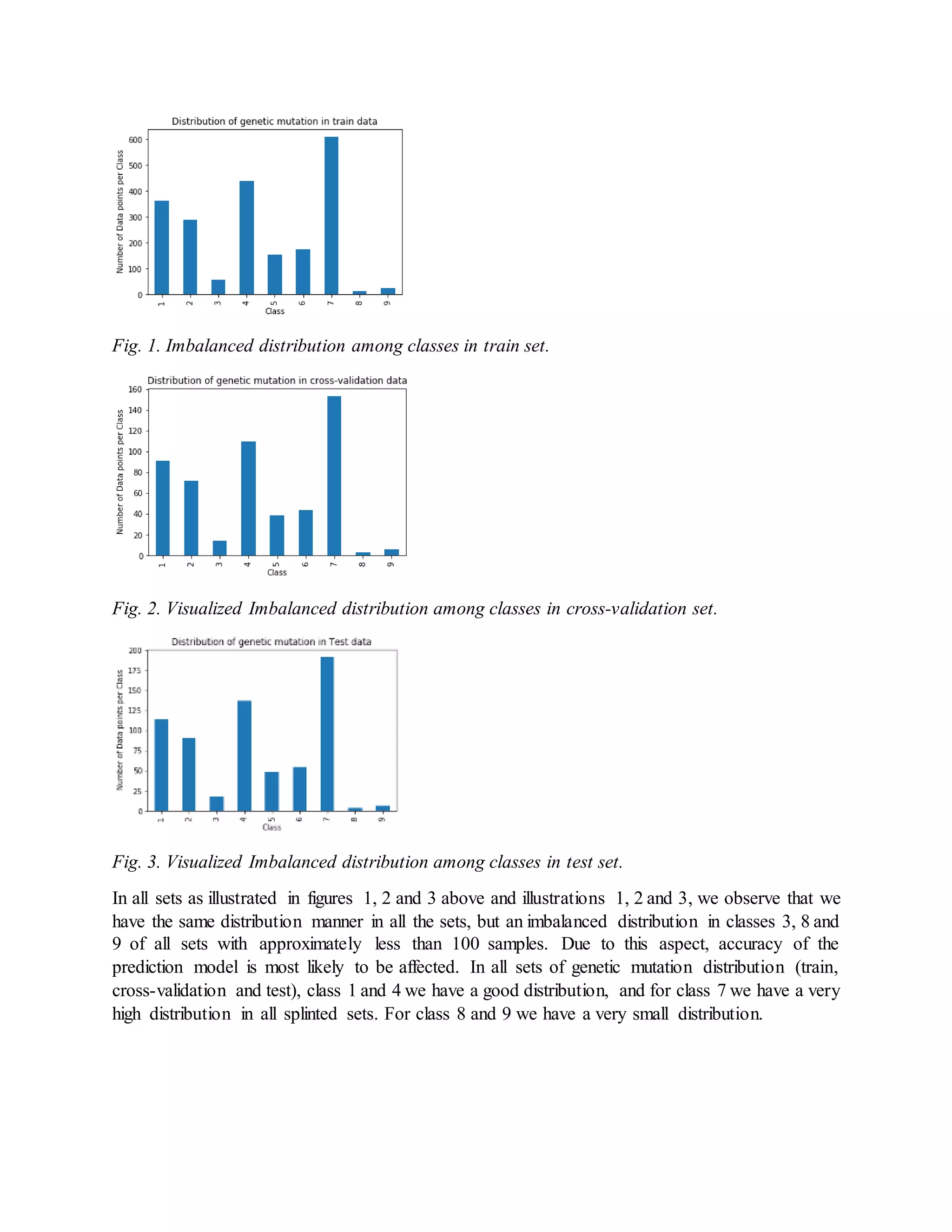
C. DATA DISTRIBUTION IN TRAIN, VALIDATION AND TEST SETS
We look into the distribution of different genetic mutation classes in train, cross-validation and
test sets in figures 1, 2 and 3 respectively.

4. Fig. 1. Imbalanced distribution among classes in train set.
Fig. 2. Visualized Imbalanced distribution among classes in cross-validation set.
Fig. 3. Visualized Imbalanced distribution among classes in test set.
In all sets as illustrated in figures 1, 2 and 3 above and illustrations 1, 2 and 3, we observe that we
have the same distribution manner in all the sets, but an imbalanced distribution in classes 3, 8 and
9 of all sets with approximately less than 100 samples. Due to this aspect, accuracy of the
prediction model is most likely to be affected. In all sets of genetic mutation distribution (train,
cross-validation and test), class 1 and 4 we have a good distribution, and for class 7 we have a very
high distribution in all splinted sets. For class 8 and 9 we have a very small distribution.

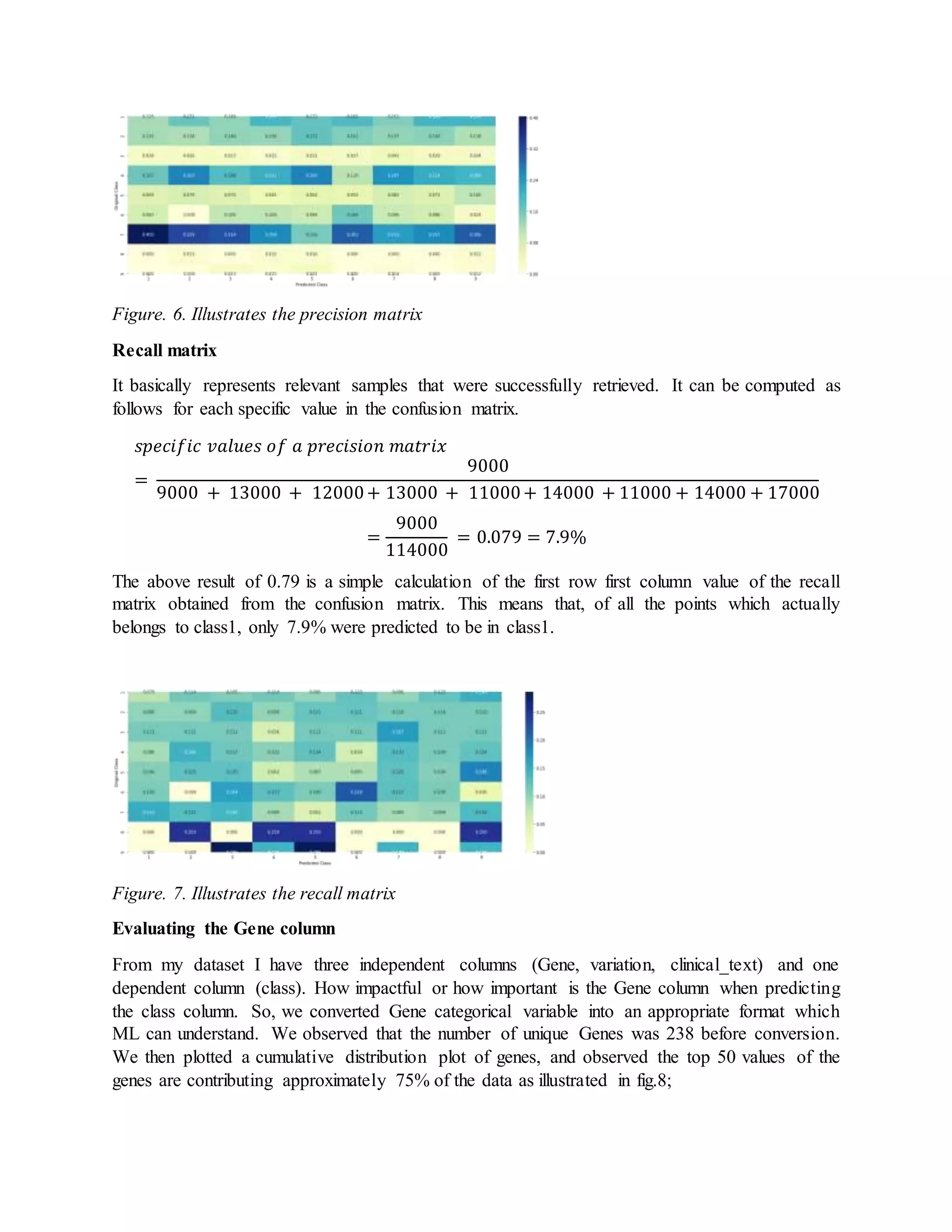
5. EVALUATION
Various ways can be used to evaluate a ML model, accuracy, area under a curve among many
other evaluation matrices. But i evaluated our model using the multi class log loss or sometimes
called the cross-entropy loss and a Confusion matrix.
LOG LOSS, MULTI CLASS LOG LOSS OR CROSS ENTROPY.
Log loss stands for logarithmic loss, its values range from 0 to ∞, it’s a loss function for
classification that quantifies the price paid for inaccuracy of predictions in classification
problems[8]. Log loss is used for binary classification algorithms (limited to only two possible
outcomes). Additionally, for a perfect model its log loss should be zero. But in real world there is
no perfect model. If more of your prediction is better, the log loss value is going to be low. And if
your prediction is ambiguous or unclear the log loss will penalize you. Therefore, the main idea
behind log loss is to keep the value low.
Log loss penalizes false classifications by taking into account the probability of classification.
Mathematical formula of log loss;
𝒍𝒐𝒈 𝒍𝒐𝒔𝒔 = −
1
𝑛
∑[𝑦𝑖 log 𝑝𝑖 + (1 − 𝑦𝑖)log(1 − 𝑝𝑖)]
𝑛
𝑖=1
Where n represents the number of samples or entities, 𝒑𝒊 represents the possible probability, 𝒚 𝒊
represents the Boolean original outcome in the i-th instance.
Multiclass log loss or cross entropy values, range from 0 to ∞, it’s a loss function for classification
that quantifies the price paid for inaccuracy of predictions in classification problems, it penalizes
false classifications used for multiclass classification.
Mathematical formula of cross entropy;
𝑪𝒓𝒐𝒔𝒔 𝒆𝒏𝒕𝒓𝒐𝒑𝒚 𝒍𝒐𝒔𝒔 = −
1
𝑛
∑ ∑ 𝑦𝑖 𝑗
𝑐
𝑗=1
𝑛
𝑖=1
log(𝑝𝑖 𝑗 )
Where c represents the number of classes, n represents the number of samples or entities, 𝒑𝒊
represents the possible probability, 𝒚 𝒊 represents the original outcome in the i-th instance. 𝒑𝒊 𝒋 is
the model’s probability of assigning label j to instance i.
BUILDING A WORST-CASE MODEL.
Accuracy ranges from 0 to 1, having an accuracy closer to 1 is great e.g. if it’s 0.95, the accuracy
will be 95% accuracy. In log loss a value can go from 0 to ∞. If the value comes out to be 0 then
that marks it to be a best model. Assuming we get a log loss value greater than 1, how can we
evaluate our model whether it’s a good or bad model. There a various method but for our case we
used a random model so called worst model. This model was created by completing some 9 random
numbers on our dataset because we have 9 classes, the sum should be equal to 1 because their sum
of probability is equal to 1. We generated the log loss for all sets (train, validation and test sets).

6. We obtain the Log loss on Cross Validation Data and Test Data using Random Model. The value
of Cross Validation is the worst log loss and if any of the models to be generated is greater than
the value of Cross Validation Data. Then it will be the worst model. Therefore, all the models to
be generated shouldn’t exceed cross validation log loss. We did the same for all the remaining sets.
This model obtained a log loss of 2.37 after then, we generated a logistic regression model so that
we can make a comparison …………………... The logistic regression log loss value returned is
compared to the random model log loss. The Logistic regression model is better in comparison to
any other model available.
After obtaining the random model we needed to see how good it was, so we developed a confusion
matrix. We passed the (original dataset and the y_prediction), this matrix is shown in figure.5;
Figure. 5. Illustrates a confusion matrix of a random built model
Our confusion matrix was of dimensional 9*9 output, the dark coloring illustrates that when the
value is high its shaded darker blue else light green color. The major diagonal elements of our
confusion matrix were meant to be high. The diagonal elements describe that there are 10 values
belonging to class 1. From the confusion matrix we formed the precision and recall matrices as
illustrated in figures 5 and 6 respectively.
Precision matrix
It’s also known as a concentration matrix. It’s used in the context of Bayesian analysis of a
multivariate normal distribution. In class 1 we have predicted values of 0.125, this value is derived
from the confusion matrix predicted value 9000 in class 1. Simple calculation of the first row first
column value of the precision matrix obtained from the confusion matrix;
𝑠𝑝𝑒𝑐𝑖𝑓𝑖𝑐 𝑣𝑎𝑙𝑢𝑒𝑠 𝑜𝑓 𝑎 𝑝𝑟𝑒𝑐𝑖𝑠𝑖𝑜𝑛 𝑚𝑎𝑡𝑟𝑖𝑥 =
9000
9000 + 9000 + 2000+12000 + 5000 +6000 +29000
=
9000
72000
= 0.125 = 12.5%
It basically means that, of all the points predicted in class1, 12.5 % actually belongs to class 1.
This happens for all values of a precision matrix.

7. Figure. 6. Illustrates the precision matrix
Recall matrix
It basically represents relevant samples that were successfully retrieved. It can be computed as
follows for each specific value in the confusion matrix.
𝑠𝑝𝑒𝑐𝑖𝑓𝑖𝑐 𝑣𝑎𝑙𝑢𝑒𝑠 𝑜𝑓 𝑎 𝑝𝑟𝑒𝑐𝑖𝑠𝑖𝑜𝑛 𝑚𝑎𝑡𝑟𝑖𝑥
=
9000
9000 + 13000 + 12000+ 13000 + 11000+ 14000 + 11000 + 14000 + 17000
=
9000
114000
= 0.079 = 7.9%
The above result of 0.79 is a simple calculation of the first row first column value of the recall
matrix obtained from the confusion matrix. This means that, of all the points which actually
belongs to class1, only 7.9% were predicted to be in class1.
Figure. 7. Illustrates the recall matrix
Evaluating the Gene column
From my dataset I have three independent columns (Gene, variation, clinical_text) and one
dependent column (class). How impactful or how important is the Gene column when predicting
the class column. So, we converted Gene categorical variable into an appropriate format which
ML can understand. We observed that the number of unique Genes was 238 before conversion.
We then plotted a cumulative distribution plot of genes, and observed the top 50 values of the
genes are contributing approximately 75% of the data as illustrated in fig.8;

8. Fig. 8: Illustrates an analysis of the distribution of genes
Before building any machine learning model, we need to convert or transform our data in a format
so that machine learning algorithm can easily take it as an input. Therefore, it’s necessary to
convert the categorical variable of the gene, and this can be perceived using two different
techniques; one-hot encoding and response encoding or mean imputation. We used both
techniques…………...
One-hot encoding and Response encoding
One-hot encoding is simply a process by which categorical variables are converted into a numeric
format that could be inputted into ML algorithms so that it does a better job in its predictions.
Categorical variables can exactly take on two values (binary variable) or take more than two
possible variables (polytomous variables). Categorical variables take on values that are names or
labels e.g. color of a dress (red, blue, green).
One-hot encoding removes the ordinary categorical column and creates new unique columns, due
to this fact it sometimes creates a problem. In case of too many unique categorical columns, One-
hot encoding that will require creation of too many unique columns hence increasing the
dimensionality of data. Basing on our data, using hot-encoding 238 new unique gene columns
were created. One-hat encoding works even if of huge dimensions logistic regression, SVM will
work very well.
Response encoding is sometimes called mean importation. Response encoding works in a way that
is replaces the categorical variables with their numerical values of mean, weight, average. In
response encoding, for row of our categorical data, we created new columns depending on the
number of dependent column (class). In response encoding, it creates number of columns
equivalent to the total number of dependent output variables. So, we basically have a small number
of columns created than in a one-hot encoding. Basing on our data, using response encoding 9 new
unique gene columns were created. For the Naive Bayes, K-NN, Random forest you have to use
the response encoding.
Laplace Smoothing and Calibrated classifier
How good is Gene column feature to predict my 9 classes?

9. One idea was to build our model having only gene column with one-hot encoder with simple model
like Logistic regression. If log loss with only one column Gene came out to be better than random
model, then this feature was important.
Previously, we had created a random model with 2.37 log loss. We now create a logic regression
model with one column called gene, using this column we shall predict the classes. If our logistic
log loss is less then that of the random model, then the gene is a good feature. We need to
understand Laplace smoothing from the Naive Bayes. It’s sometimes called editing smoothing and
helps to control the bias and variance made by ML model. We used calibrated classifier when
building our model. Calibrated classifier can be explained in a way that assuming your having an
input xi and you feed it to the model to output a value yi, the output (yi) is considered not to be a
probabilistic value. So, the output value is again built with a classifier called a calibrated classifier
which can be sigmoid function or any advanced level function like isotonic. When the output is
fed into the calibrated classifier it will then return a probabilistic value.
We built a model only considering the gene column, we created a logistic regression using a
Stochastic Gradient Descent (SGD) classifier, also used a calibrated classifier. A hyperparameter
will also be required, I also used a one-hat encoding. We obtained different log loss values of the
different hyperparameters. Illustration below in figure ….. for the log loss values.
Figure. …. Illustrates hyperparameter values and its log loss values of the gene column.
We observe that we have a minimum log loss at an alpha value of 0.0001, as also illustrated in
figure…. Illustrated below.
The gene column will be very necessary since it is providing a very small log loss as compared to
that outputted by the random model. We also got the log loss of the train, validation and test sets
as illustrated below.
Figure. …. Illustrates log loss of the train, cross validation and test sets.

10. We observed that the log loss values outputted by the logistic regression model are small as
compared to those outputted by the random model, therefore the gene column has a great impact
due to that factor.
Evaluating the Variation column
From the new formulated dataset there are three independent columns (Gene, variation,
clinical_text) and one dependent column (class). Variation is also a categorical variable so we dealt
with it in the same way like we did for Gene column. We again got the one hot encoder and
response encoding variable for variation column. Variation has 1941 number of unique variations.
Figure…… illustrates the cumulation distribution of variations.
We then plotted a cumulative distribution plot of variations as illustrated in figure…. For the one-
hot encoding we obtained 1970 new formed columns, and with response encoding returned
basically nine particular columns for the variation. We then build our model with only the variation
column in the same previous way as that of the gene column. The following values where obtained
as shown below;
Figure. …. Illustrates hyperparameter values and its log loss values of the variations column.
From the above illustration, we observed that the minimum log loss is at a hyperparameter of
0.001. this is also illustrated in below;
The log loss values of all sets were computed, the output log loss values are shown below figure…..
we observe that the best value of alpha the log loss for test is approximately lesser as compared to
the random model, therefore, this column wont be considered in the final model……..

11. Evaluating the Text column
For the text data column, we obtained the total number of unique words in the train data which
was 53451. We used the response encoding for the text features, and even normalized every feature
using one-hot encoding. Sorted our text, and we where able to know the number of words for a
given frequency i.e. 3: 5361 denotes that there are 5361 values that are occurring 3 times and so
no. we then built our model with only the text column data. As before on other columns, we built
our model using logistic regression, calibrated classifier, one-hot encoding, we got the following
output log-loss values for the hyperparameter illustrated in figure…….
Figure. …. Illustrates hyperparameter values and its log loss values of the text column.
The minimum log loss is mapped at an alpha point of 0.001, and this can be further be elaborated
by a graph as illustrated in figure …. below;
We compute the log loss for all the three data sets, the log loss for the test set is 1.12, which is
much better in comparison to that of the variation set. Therefore, this column is also critical.
Accordingly, all the three independent columns (gene, variation and text) are highly and extremely
important in the building of our models (Naive Bayes and K-NN models).
Data preparation for the machine learning models
Here we formulated three functions that can be recalled at any time, first, was a report_log_loss
function that reports back the log loss since we are to build various models like Naive Bayes and
K-NN. Second, to a plot_confusion_matrix function that returns a precision, recall and accuracy
matrices, so that our models can predict. Third, to get_impfeature_names that will be used just in
the Naive Bayes to check whether the feature is present in the text or not.
Combining all the three columns

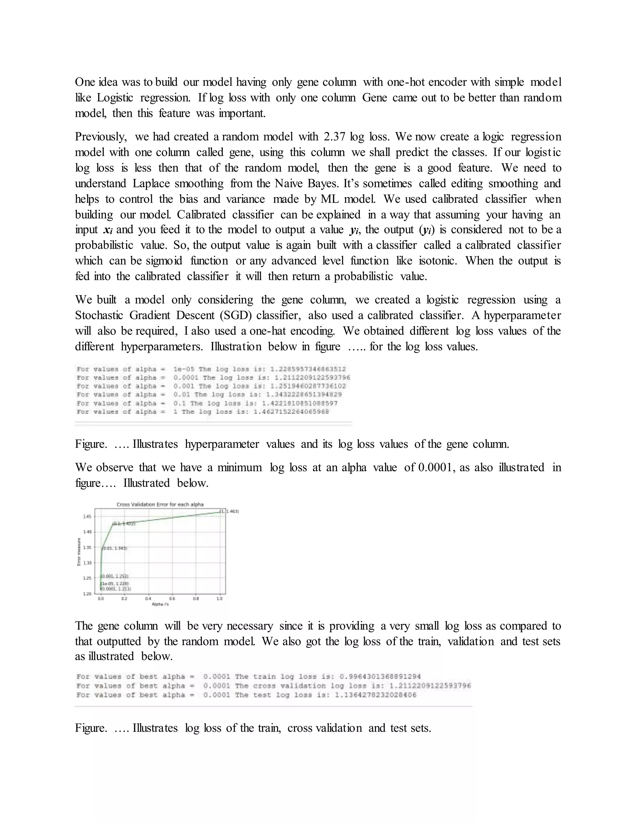
12. So, we need to bring all the three independent columns together to work and build the model (gene,
variation and the text). Using both one-hot encoding and response encoding we obtained the
following shapes for all three kinds of datasets as illustrated in the figures….. below;
we observe that we got much greater number of columns when using the one-hot encoding with
values of 55659 columns since we have 18553 number of columns in each set of the three sets.
We have 27 columns when using the response encoding feature because each set has 9 unique
classes.
Building the machine learning models
I. Naive Bayes Classification Model.
Since we have a lot of text data, we decided to start building our model with Naive Bayes
classifier. Naive Bayes is a probabilistic classifier based on applying the Bayes theorem[9], it’s
also known as simple Bayes and independence Bayes. We built our model using all the three
independent columns (gene, variation and text columns).
Bayes theorem:
𝑃( 𝐴𝐵) =
𝑃( 𝐵𝐴) ∗ 𝑃(𝐴)
𝑃(𝐵)
Using Bayes theorem, we can find the probability of A happening, given that B has occurred.
Accordingly, B is the evidence and A is the hypothesis. The assumption made are, the predictors
or features are independent, (presence of one particular feature does not affect the other). Naive
Bayes classifier converge quicker than any other discriminative models like logistic regression, so
you it requires a small amount of training data[10].
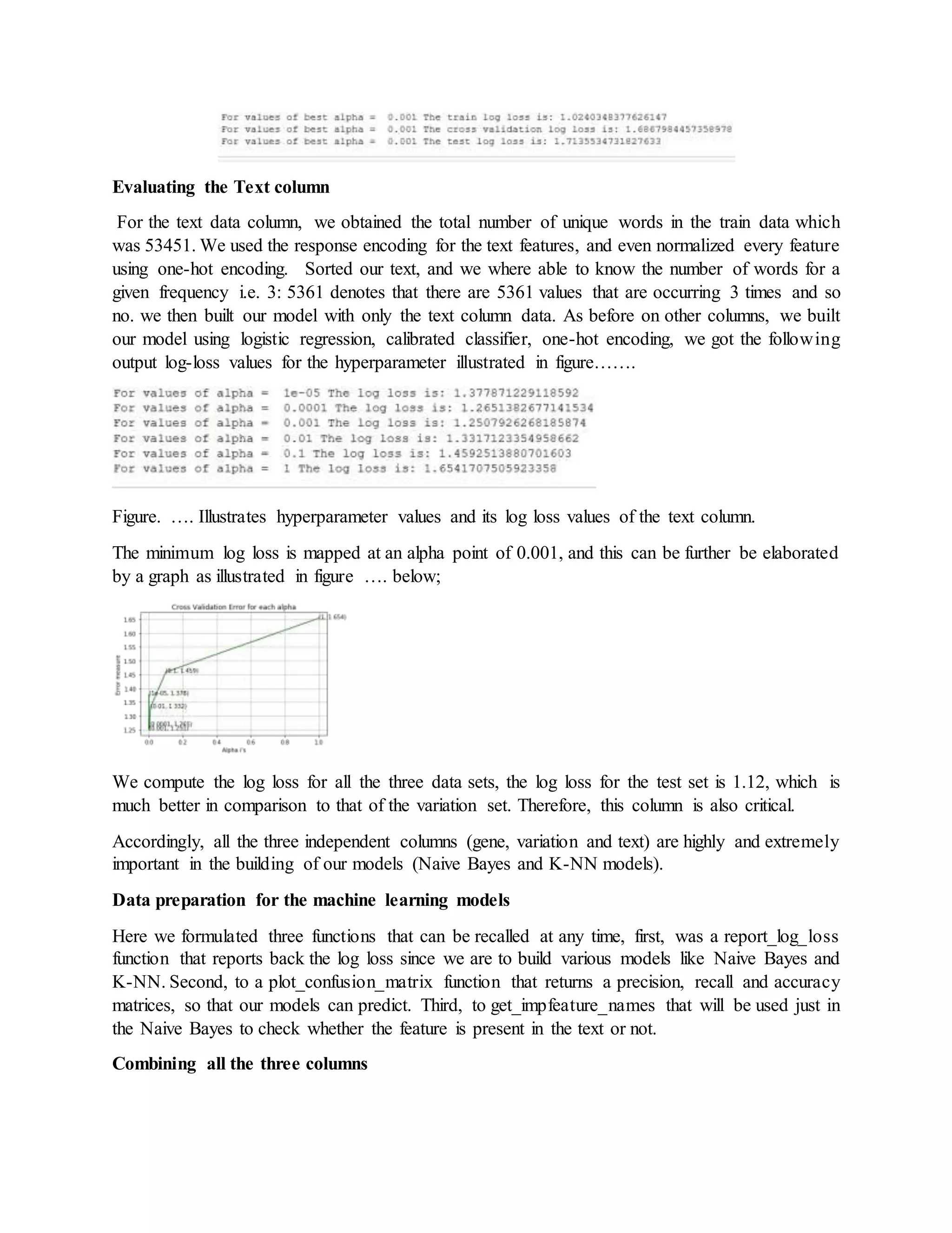
We used the alpha and the multinomial Naive Bayes classifier for multiclass classification. We fit
the model using the one-hot encoding. We then get the log loss of alpha values with a minimum
value of 1.27 at alpha 0.1 as illustrated in the figure….. shown below;

13. We then used this minimum value on the test data and our log loss came out to be 1.24 as illustrated
in the figure….. below;
From our train set we have a log loss value of 0.94 and for the test set its 1.24, the difference
between these values is 0.3 which is reasonable, but if there was a big value between the train set
and the test set, this assumes that there was an overfitting on the training set.
Using a Confusion matrix, it describes the performance of our model through obtaining the
accuracy, precision and recall as shown in the figure below;
Figure. Confusion matrix output values of Naive Bayes model
Our confusion matrix is giving us good results, because most of the minor or wrong places they
are filled with zeros, and in the major diagonal we have high value results or outputs of our model.
However, we have some values in the minor areas and we term them as errors or wrongly classified
points, but the precision matrix gives us some good results as shown below in figure…..

14. Figure. ….. Illustrates a precision matrix output values of a Naive Bayes model
However, the precision matrix gives us a good idea because ideally, we want the binomial value
to be one. There is a high confusion happening between predicted class 2 and original class 7,
predicted class 3 and original class 7 among few more others. This clarifies that we can’t come up
with a perfect model.
Also in figure…..below we have a recall matrix. Few places have wrongly classified points. There
is a confusion in the predicted class 2 and original class 8 plus some few other points. This also
clarifies that we can’t come out with a perfect model
Figure. ….. Illustrates a recall matrix output values of a Naive Bayes model
Interpretability of our model
Why is this model (Naive Bayes) predicting these results? To answer this question, we used a
getImpfeatureNames, we passed to it a data point and it predicted class 7 and the actual class 7 as
shown below;
The probability of class7 is the highest true prediction class with a value of 0.6289 (63%),
according to the output results of our model. The second value close to the highest is 0.0916

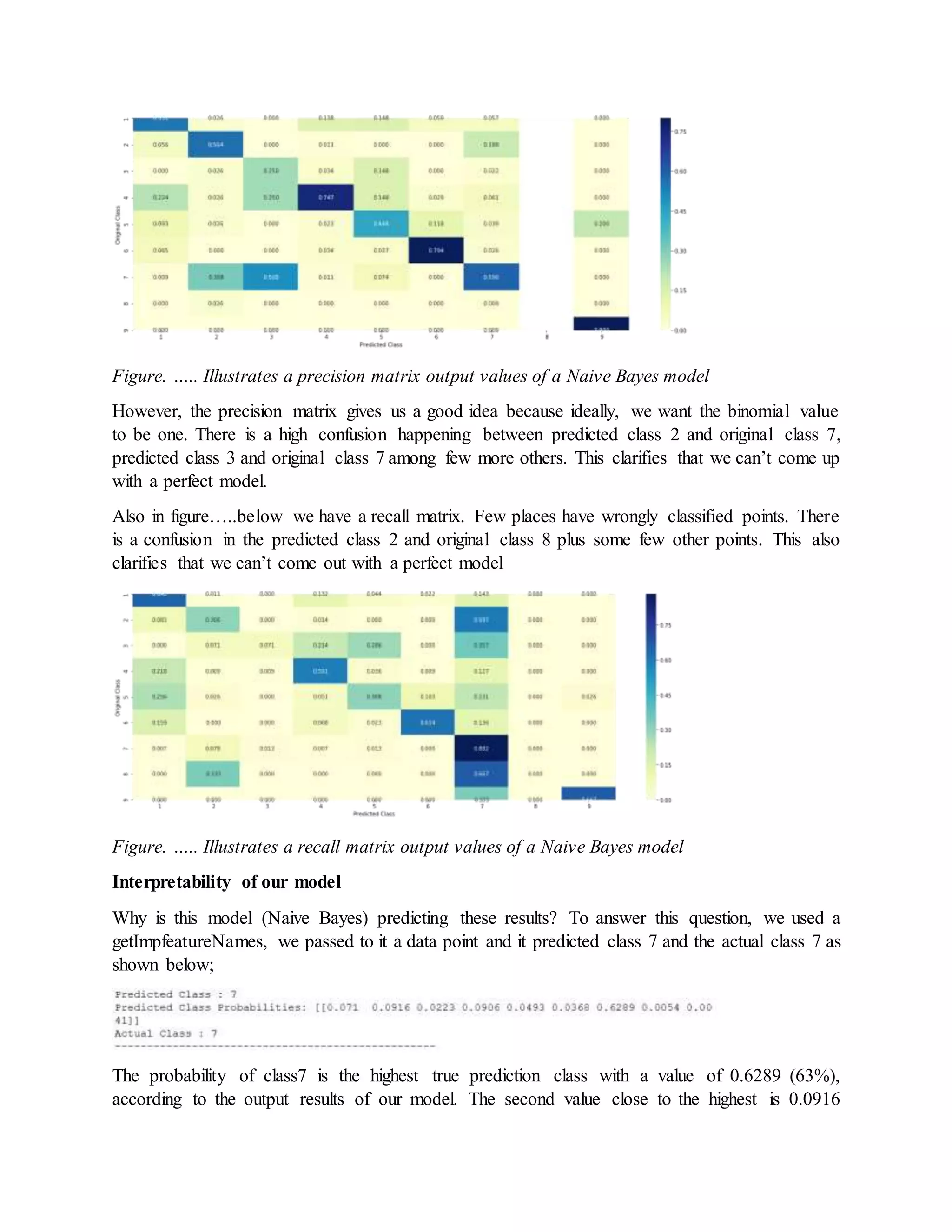
15. (9.2%), this is a big difference, so there is no confusion hence the model is working very well. And
this answers the above question.
The accuracy of our model;
𝐴𝑐𝑐𝑢𝑟𝑎𝑐𝑦 = 1 − 𝑁𝑢𝑚𝑏𝑒𝑟 𝑜𝑓 𝑚𝑖𝑠𝑐𝑙𝑎𝑠𝑠𝑖𝑓𝑖𝑒𝑑 𝑝𝑜𝑖𝑛𝑡𝑠
= 1 − 0.3890977443609023
= 0.610902255
𝐴𝑐𝑐𝑢𝑟𝑎𝑐𝑦 = 61.1%
This was quite a good accuracy according to the problem we were solving. Therefore, the output
results for our model were quite good with such an impressive percentage of accuracy.
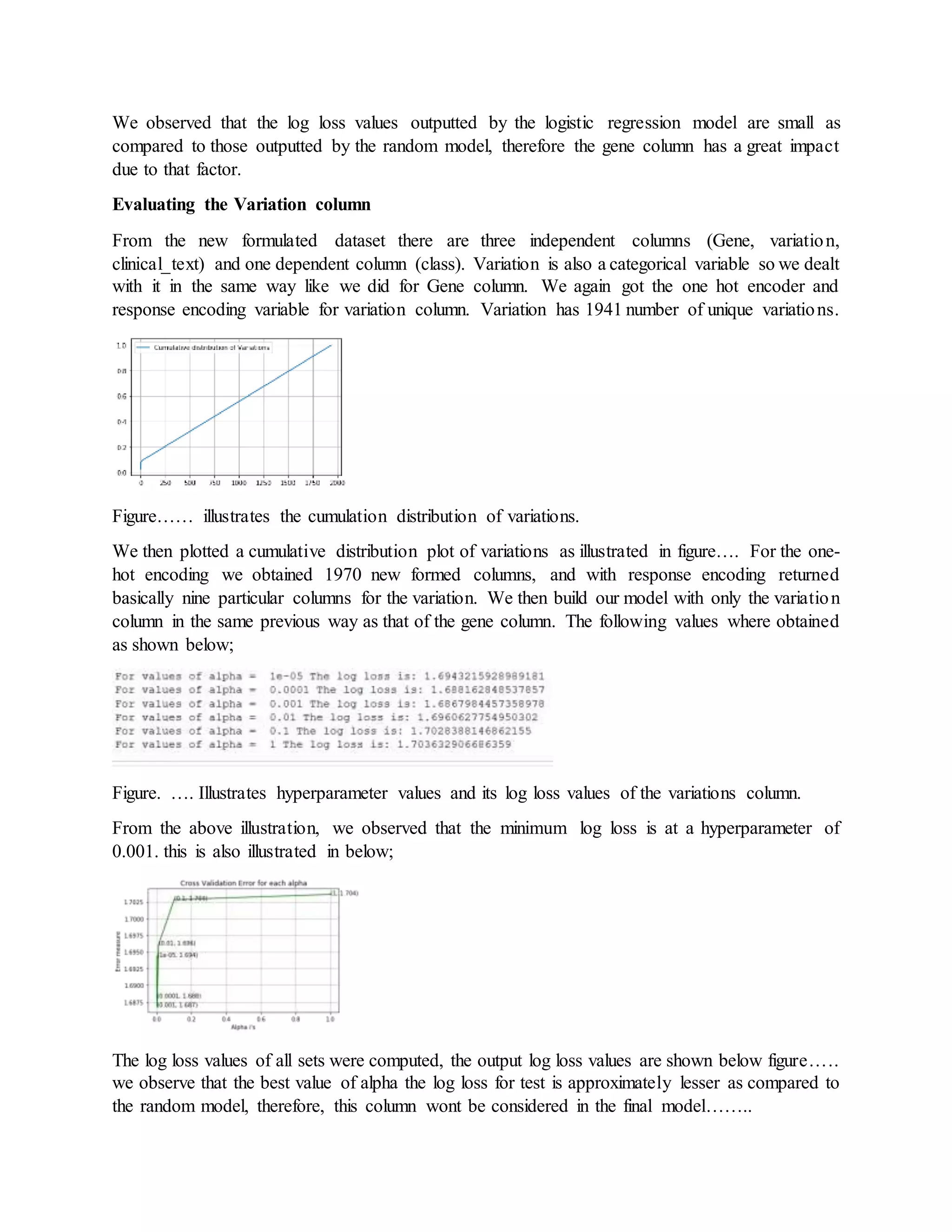
II. Logistic regression
Logistic regression describes data, and explains the relationship between one dependent binary
variable and one or more independent categorical variables sometimes called the target[11]. There
are basically three types of logistic regression; binary, multinomial and ordinal LR. Since the
problem we are solving it a multinomial problem we shall concentrate on multinomial LR.
We are going to do over sampling because in most classes we had much data and in some few
classes we had less data, due to this factor it can affect the performance of our model. We shall try
to balance the classes. Here we try to demonstrate our model with balanced classes.
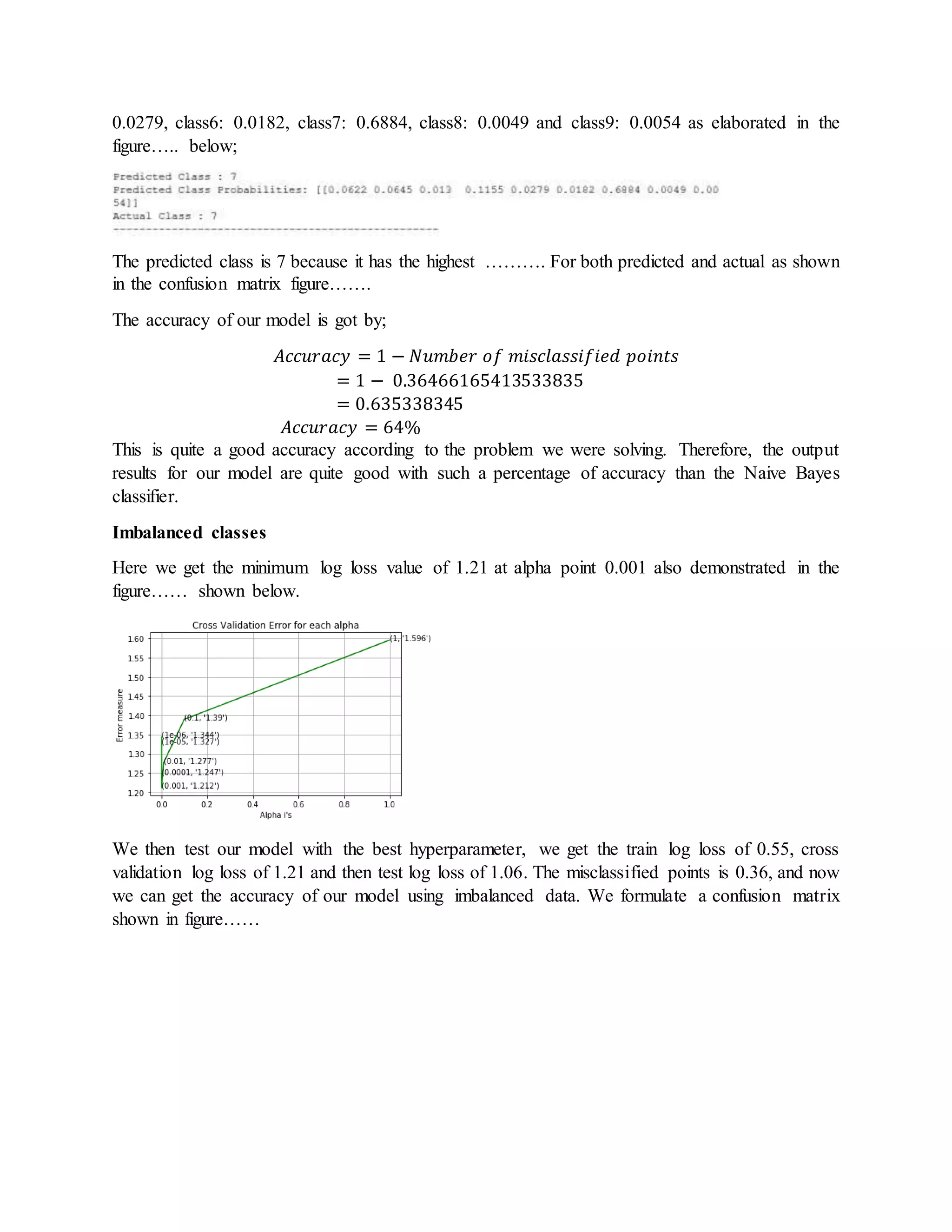
Balanced classes
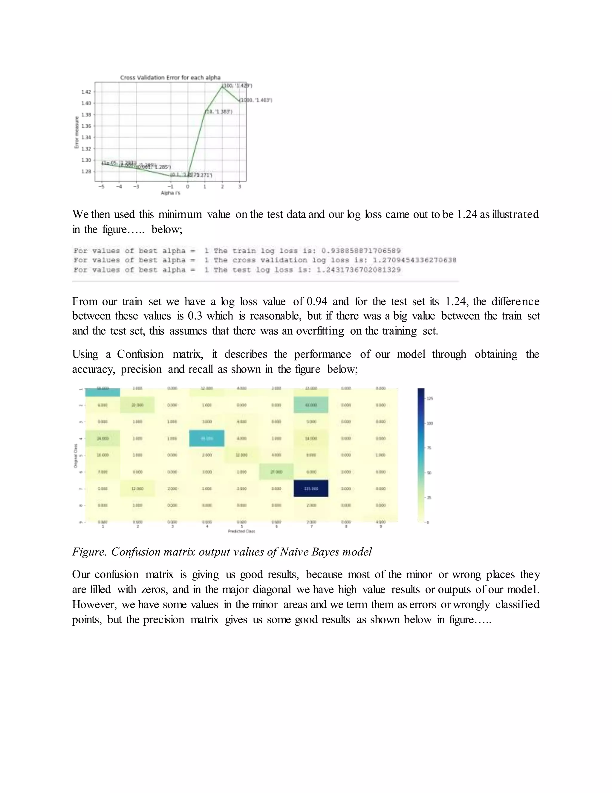
Using the SGD Classifier, we balanced our classes. We got the minimum log loss value of 1.19 at
alpha point 0.001 also demonstrated in the figure…… shown below. interpretability
We tested our log loss minimum value on the testing data using the alpha value. Our outputted log
loss value was 1.19 and the misclassified points was 0.36. From these results we can tell the
accuracy of our model. The performance of our classification model on the testing dataset was
described by a confusion matrix shown in figure…… below;

16. Figure. ….. Illustrates a confusion matrix describing LR model
We also formulate the precision and recall matrices as show in the figures………… show
respectively.
Figure. ….. Illustrates a precision matrix.
Figure. ….. Illustrates a recall matrix.
LR is quite good in terms of interpreting the results, it looks at the weights and coefficients,
interprets them and gives you the results. Using the function get_impfeature_names we can predict
the class with the highest, class1: 0.0622, class2: 0.0645, class3: 0.013, class4: 0.1155, class5:

17. 0.0279, class6: 0.0182, class7: 0.6884, class8: 0.0049 and class9: 0.0054 as elaborated in the
figure….. below;
The predicted class is 7 because it has the highest ………. For both predicted and actual as shown
in the confusion matrix figure…….
The accuracy of our model is got by;
𝐴𝑐𝑐𝑢𝑟𝑎𝑐𝑦 = 1 − 𝑁𝑢𝑚𝑏𝑒𝑟 𝑜𝑓 𝑚𝑖𝑠𝑐𝑙𝑎𝑠𝑠𝑖𝑓𝑖𝑒𝑑 𝑝𝑜𝑖𝑛𝑡𝑠
= 1 − 0.36466165413533835
= 0.635338345
𝐴𝑐𝑐𝑢𝑟𝑎𝑐𝑦 = 64%
This is quite a good accuracy according to the problem we were solving. Therefore, the output
results for our model are quite good with such a percentage of accuracy than the Naive Bayes
classifier.
Imbalanced classes
Here we get the minimum log loss value of 1.21 at alpha point 0.001 also demonstrated in the
figure…… shown below.
We then test our model with the best hyperparameter, we get the train log loss of 0.55, cross
validation log loss of 1.21 and then test log loss of 1.06. The misclassified points is 0.36, and now
we can get the accuracy of our model using imbalanced data. We formulate a confusion matrix
shown in figure……

18. Also we see that the predicted class is 7 and the actual class is 7
IV. Comparison between Naive Bayes and Logistic Regression Classification Models
TABLE 1. COMPARISION BETWEEN PERFOMANCES OF THE NAIVE BAYES AND
LOGISTIC REGRESSION CLASSIFICATION MODELS
Train Cross-validation Test Misclassified Accuracy
Naive Bayes 0.94 1.27 1.24 0.39 0.61
Logistic
Regression
0.55 1.19 1.05 0.36 0.64
For the Naive Bayes ML model, in the train set we have a log loss value of 0.94, in a cross-
validation the log loss is 1.27 and on the testing data the log loss is 1.24, its misclassified points is
0.39 making an accuracy score of the model to be 61%. Under the logistic regression, in the train
set we have a log loss value of 0.55, in a cross-validation the log loss is 1.19 and on the testing
data the log loss is 1.05, its misclassified points are 0.36 making an accuracy score of the model
to be 64%. The evaluation criteria is based on the principle of minimum error, and from our table
about 1.05 is the minimum log loss under our test set. Therefore, according to the results from both
models, the multinomial logistic regression has a better predictive ability than the Naive Bayes,
due to the less log loss value on the test set and the smaller number of misclassified points.
This paper is organized as follow: Section II covers K-Nearest Neighbor algorithm, section III
describes Naive Bayes classifier. Finally, section IV covers the comparative analysis of these
algorithm followed by results of implementation and conclusions.

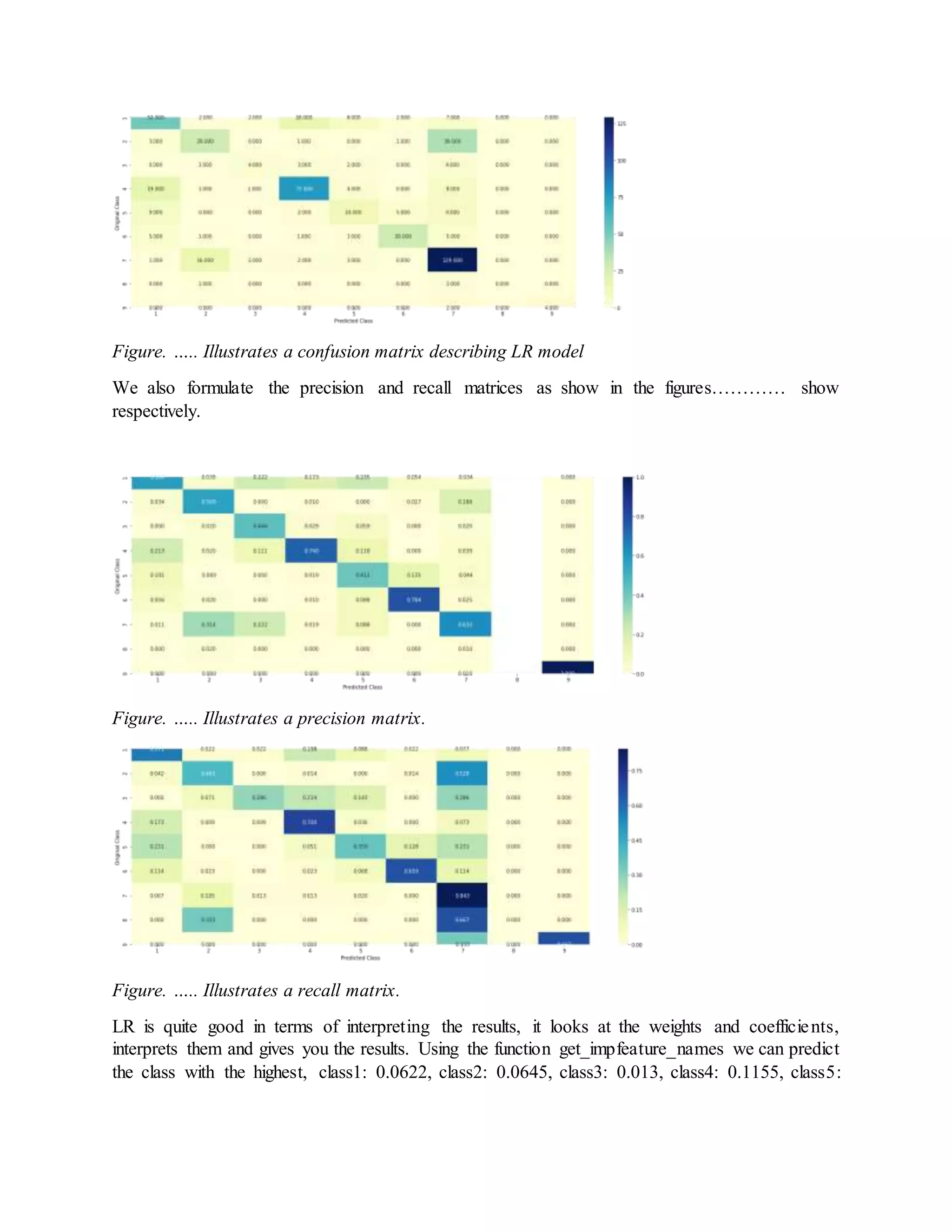
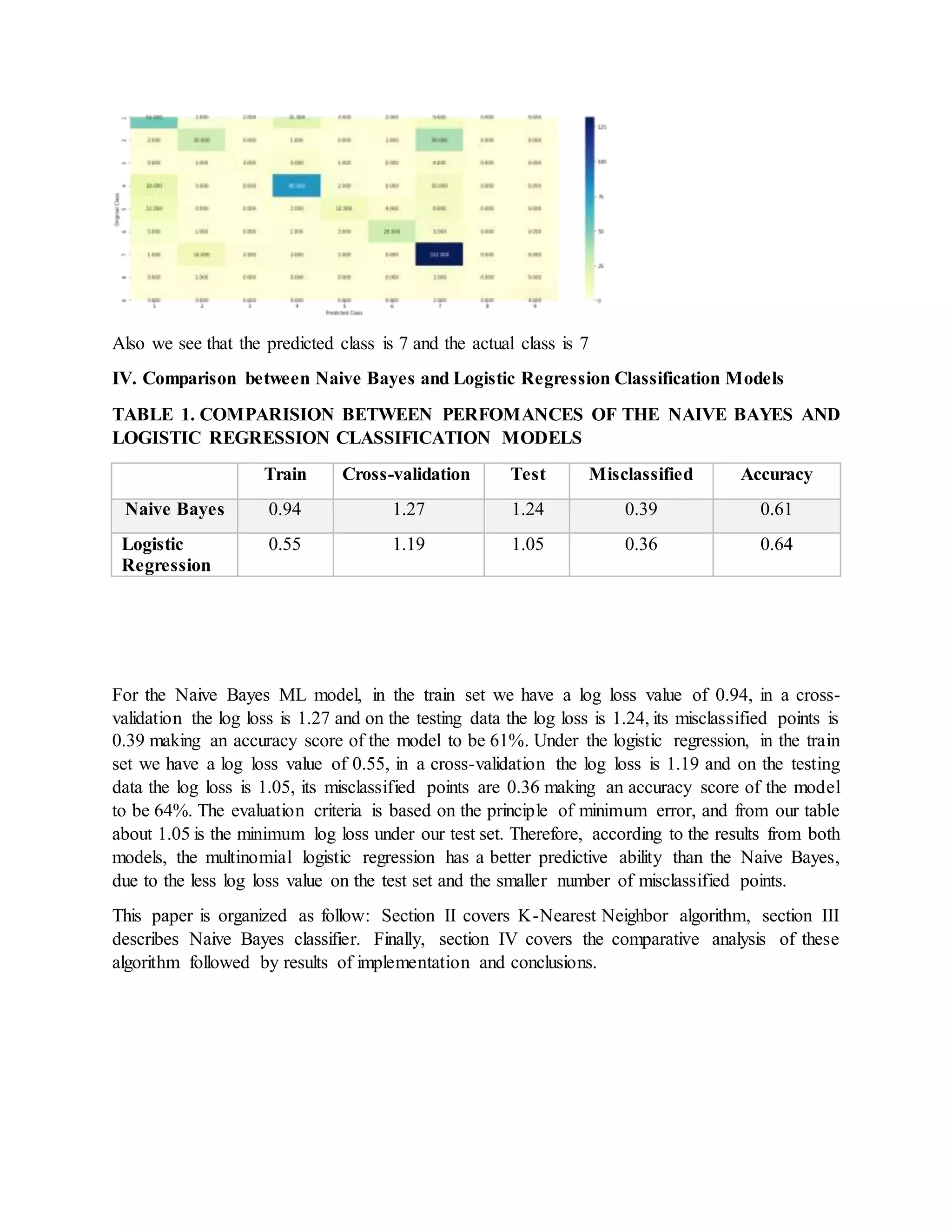
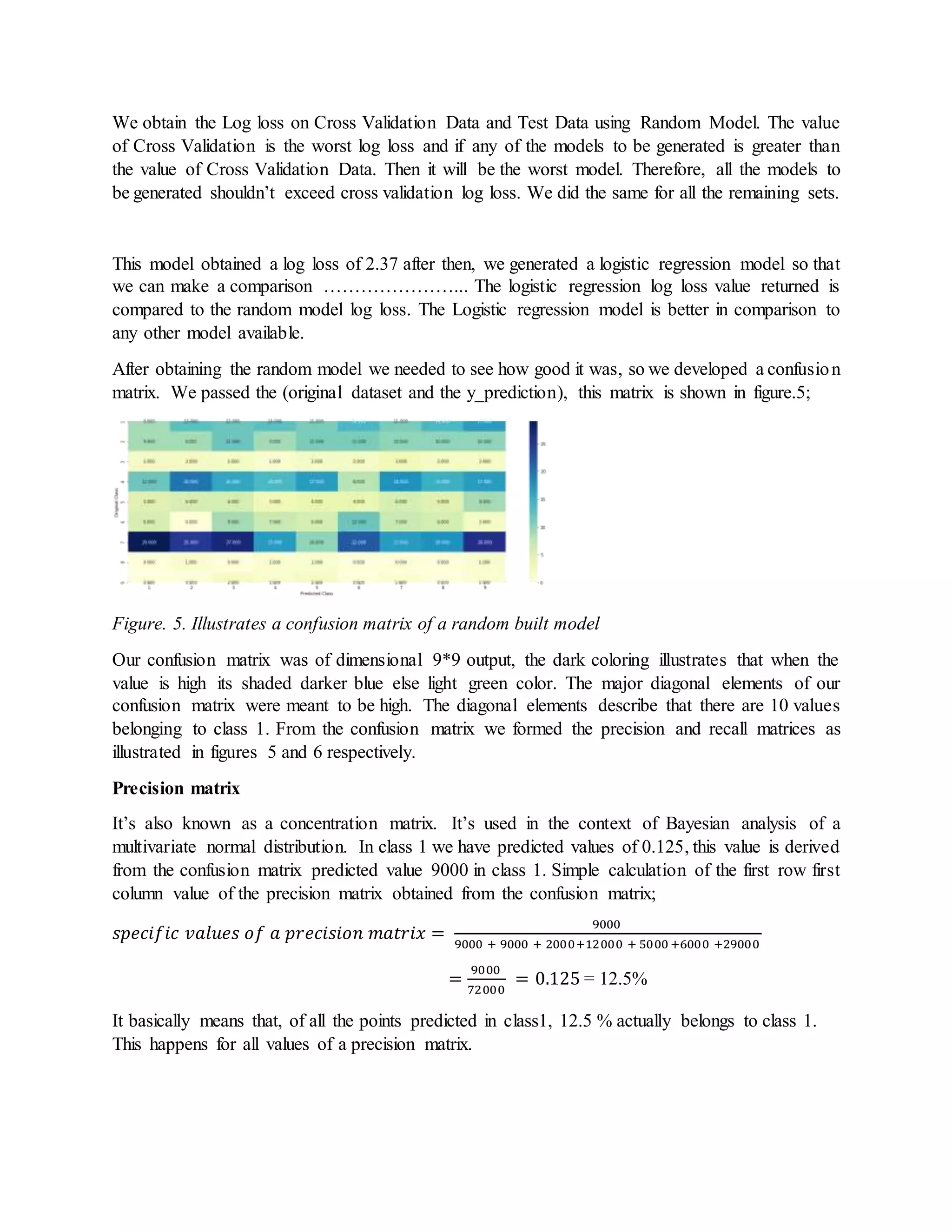
19. Discussion
The preliminary results obtained from our study really verified the possibility of implanting
machine learning algorithms (Naive Bayes and Multinomial Logistic Regression) into
classification of Genetic Mutations, which is text-based and probabilistic classification problem.
This reduce deadly manual work and accelerate the progression in analyzing cancer roots. In this
section, we will further interpret this project based on the analysis of our results.
Firstly, Analyzed the shapes of our datasets, understood the independent and dependent variables
and the kind of data present in target of dependent column. It was discrete data therefore, it was a
classification problem because of the multiple discrete outputs (classes 1 to 9).
Secondly, since we had medical text data, so we preprocessed it into a good format so that ML
algorithm can understand and input it. We merged our two data sets into one dataset, then did some
imputation since we had some missing values, we then splinted our data into three sets (Train 60%,
Cross-validation 20% and Test 20%).
Thirdly, we performed random sampling since our classes (1-9) had imbalanced data so as to
improve the performance of our model.
Fourthly, we evaluated each column independently to make sure that its relevant for our target
variable (class column). Some columns had categorical data so, we converted this categorical data
using one-hot encoding technique. Finally, we observed that all the independent columns were
relevant.
Fifthly, we performed over sampling to reduce bias due to the highly twisted distributed data. And
then finally, regarding the performances of the two classification models Logistic regression
performed better than the Naive Bayes ML algorithm. Since it had fewer misclassified datapoints
and a high degree of accuracy than the Naive Bayes classifier.
Conclusion
From survey and analysis on comparison among data mining classification algorithms (Naive
Bayes and Multinomial logistic regression), it shows that logistic regression algorithm is more
accurate and has less error rate and it’s an easier algorithm as compared to Naive Bayes. When
modeling Logistic regression, we used balanced data and so we may need to also use imbalanced
data and try to compare the results obtained.
References.
[1] F. Okongo, D. M. Ogwang,B. Liu, and D. MaxwellParkin, "Cancer incidence in Northern Uganda
(2013–2016)," International journal of cancer, vol. 144, no. 12, pp. 2985-2991, 2019.
[2] M. Verma, "Personalized medicine and cancer," Journal of personalized medicine, vol. 2, no. 1,
pp. 1-14, 2012.
[3] G. Li and B. Yao, "Classification of Genetic Mutations for Cancer Treatment with Machine
Learning Approaches," InternationalJournalof Design,Analysisand ToolsforIntegratedCircuits
and Systems, vol. 7, no. 1, pp. 63-67, 2018.

20. [4] A. Holzinger, "Trends in interactive knowledge discovery for personalized medicine: cognitive
science meets machine learning," The IEEE intelligent informatics bulletin, vol. 15, no. 1, pp. 6-
14, 2014.
[5] M. W. Libbrecht and W. S. Noble, "Machine learning applications in genetics and genomics,"
Nature Reviews Genetics, vol. 16, no. 6, pp. 321-332, 2015.
[6] A. E. Maxwell, T. A. Warner, and F. Fang, "Implementation of machine-learning classification in
remote sensing: An applied review," International Journal of Remote Sensing, vol. 39, no. 9, pp.
2784-2817, 2018.
[7] Kaggle. "Personalized Medicine: Redefining Cancer Treatment." Kaggle.
https://www.kaggle.com/c/msk-redefining-cancer-treatment (accessed.
[8] V. Vovk, "The fundamental nature of the log loss function," in Fields of Logic and Computation
II: Springer, 2015, pp. 307-318.
[9] H. Padmanaban, "Comparative analysis of Naive Bayes and tree augmented naïve Bayes models,"
2014.
[10] Z. K.Senturk and R.Kara,"Breast cancerdiagnosis via data mining: performance analysis of seven
different algorithms," Computer Science & Engineering, vol. 4, no. 1, p. 35, 2014.
[11] R. E. Wright, "Logistic regression," 1995.