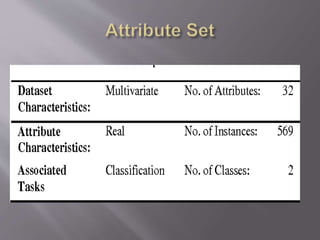
Cancer is a disease caused by abnormal cell growth and can affect different cell types. This paper focuses on breast cancer, which is classified based on the type of affected cell. There are several risk factors that can increase the likelihood of developing cancer, including gender, age, genetics, family history, weight, alcohol use, and smoking. The dataset used contains information from 569 breast cancer cases, including demographic and cell feature data. Machine learning algorithms like decision trees can be applied to build models for diagnosing breast cancer based on these attributes with up to 96.46% accuracy.

1. Cancer is a disease in which abnormal cells divide uncontrollably and destroy body
tissues. The human body is comprises of million of cells each with its unique function.
When there is unregulated growth of any of these cells termed as Cancer.
Cancer is classified by the type of cell is affected and more than 200 types of
cancer are known. This paper is focused on Breast Cancer. Cancer is the name given to a
collection of related disease.
There are some factors which cause cancer-
1. Gender
2. Age
3. Genetic Factor
4. Family History
5. Over weight
6. Alcoholic
7. Smoking

2. The dataset used in this story is publicly available and was created
by Dr. William H. Wolberg, physician at the University Of
Wisconsin Hospital at Madison, Wisconsin, USA.
Reference:
http://archive.ics.uci.edu/ml/datasets/breast+cancer+wisconsin+%28diagn
ostic%29
Attribute Information
1.ID Number
2.Diagnosis(M=Cancerous, B=Non Cancerous)

3. Ten real-valued features are computed for each cell nucleus:
1.radius (mean of distances from center to points on the perimeter)
2.texture (standard deviation of gray-scale values)
3.perimeter
4.area
5.smoothness (local variation in radius lengths)
6.compactness (perimeter² / area — 1.0)
7.concavity (severity of concave portions of the contour)
8.concave points (number of concave portions of the contour)
9.symmetry
10.fractal dimension (“coastline approximation” — 1)
The mean, standard error and “worst” or largest (mean of the three
largest values) of these features were computed for each image, resulting in 30
features. For instance, field 3 is Mean Radius, field 13 is Radius SE, field 23 is
Worst Radius.

5. We can observe that the data set contain 569 rows and 32 columns.
‘Diagnosis’ is the column which we are going to predict , which says if
the cancer is M = malignant or B = benign.
1 means the cancer is malignant and 0 means benign. We can
identify that out of the 569 persons, 357 are labeled as B (benign) and
212 as M (malignant).
Visualization of data is an imperative aspect of data science. It
helps to understand data and also to explain the data to another
person.

6. Categorical data are variables that contain label values rather than
numeric values.
The number of possible values is often limited to a fixed set.
For example, users are typically described by country, gender, age group
etc.
In this process we give a fixed numeric values to label values.
M= Cancerous changed to 1.
B= Non Cancerous changed to 0.
Splitting the data set –
The data we use is usually split into training data and test data. The
training set contains a known output and the model learns on this data in
order to be generalized to other data later on. We have the test dataset (or
subset) in order to test our model’s prediction on this sub

7. In this phase , we use the data transformation techinique
for scaling our data into some scale of either 0-100 or 0-1.
Most of the times, your dataset will contain features highly
varying in magnitudes, units and range. But since, most of the
machine learning algorithms use Euclidian distance between two
data points in their computations.
We need to bring all features to the same level of
magnitudes. This can be achieved by scaling.
There are various transformation techniques is available in data
mining-
1.Min – Max Scaling
2. Z-Score Scaling

8. In this phase, we use Data Mining Algorithms on our
Data set Algorithm can be classified into two groups :
Supervised learning : Supervised learning is a type of
system in which both input and desired output data are
provided. Input and output data are labeled for
classification to provide a learning basis for future data
processing.
Supervised learning problems can be further grouped
into Regression and Classification problems.

9. •A regression problem is when the output variable is a
real or continuous value, such as “salary” or “weight”.
•A classification problem is when the output variable is a
category like filtering emails “spam” or “not spam”
Unsupervised Learning : Unsupervised learning is
the algorithm using information that is neither classified nor
labeled and allowing the algorithm to act on
that information without guidance.
In our dataset we have the outcome variable or Dependent
variable
i.e. Y having only two set of values, either M (Malign) or B
(Benign)
So we will use Classification algorithm of supervised learning.

10. Decision tree is a classifier that is expressed as a recursive partition of the
instance space. It creates a predictive model, which maps observations about a
node to conclusions about the nodes’ target value. In a tree structure leaves
represent the class labels and branches represent conjunctions of feature leading
to the class labels. Figure shows the illustrated example of binary decision tree.

11. PROCEDURE:
1. Acquire dataset from Hospital Breast Cancer datasets.
2. Pre-process data for applying J48 decision tree data mining technique. a.
Remove Sample Code Number from attribute list b. Numeric to
nominal type of data conversion of Class attribute. (2 – Benign, 4-
Malignant)
3. Pre-processed dataset uploaded in sklearn in python toolkit for analysis.
4. Information Gain algorithm applied in sklearn of respective attributes
record
5. Decision Tree J48 algorithm implemented, generating a decision tree
with leaf nodes as the class label (benign and malignant).
6. Diagnosis of new patients is achieved by cross referencing new attribute
values in the decision tree and following path till the leaf node reached
which would either specify benign or malignant tumor.

13. By using Decision Tree Method for Classification of our data set it is giving
the accuracy of approximately 96.46% which is a good result for small data
set. We can also gain higher accuracy by adding more information of about
the data set.
The automatic diagnosis of Breast cancer is an important real world medical
problem. Detection of breast cancer in its early stages is the key for treatment.
This paper shows how decision trees are used to model actual diagnosis of
Breast cancer for local and systematic treatment, along with presenting other
techniques that can be applied.
Experimental results show the effectiveness of the proposed model.
The performance of decision tree technique was investigated for the Breast
cancer diagnosis problem.