Download as PDF, PPTX
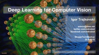


![A bit of history:
Neurocognitron
[Fukushima 1980]
“sandwich” architecture (SCSCSC…)
simple cells: modifiable parameters
complex cells: perform pooling](https://image.slidesharecdn.com/deeplearning-161020090534/85/Deep-Learning-STM-6-7-320.jpg)
![Gradient-based learning applied to
document recognition
[LeCun, Bottou, Bengio, Haffner 1998]
LeNet-5
https://www.youtube.com/watch?v=FwFduRA_L6Q](https://image.slidesharecdn.com/deeplearning-161020090534/85/Deep-Learning-STM-6-8-320.jpg)


![ImageNet Classification with Deep
Convolutional Neural Networks
[Krizhevsky, Sutskever, Hinton, 2012]
“AlexNet”
Deng et al.
Russakovsky et al.
NVIDIA et al.](https://image.slidesharecdn.com/deeplearning-161020090534/85/Deep-Learning-STM-6-11-320.jpg)


![[224x224x3]
f 1000 numbers,
indicating class scores
Feature
Extraction
vector describing
various image statistics
[224x224x3]
f 1000 numbers,
indicating class scores
training
training](https://image.slidesharecdn.com/deeplearning-161020090534/85/Deep-Learning-STM-6-15-320.jpg)


![[224x224x3]
f 1000 numbers,
indicating class scores
training
Only two basic operations are involved throughout:
1. Dot products w.x
2. Max operations
parameters
(~10M of them)](https://image.slidesharecdn.com/deeplearning-161020090534/85/Deep-Learning-STM-6-18-320.jpg)


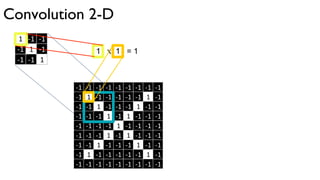


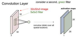

![32
32
3
Convolution Layer
activation maps
6
28
28
For example, if we had 6 5x5 filters, we’ll get 6 separate activation maps:
We processed [32x32x3] volume into [28x28x6] volume.
Q: how many parameters would this be if we used a fully connected layer instead?](https://image.slidesharecdn.com/deeplearning-161020090534/85/Deep-Learning-STM-6-44-320.jpg)
![32
32
3
Convolution Layer
activation maps
6
28
28
For example, if we had 6 5x5 filters, we’ll get 6 separate activation maps:
We processed [32x32x3] volume into [28x28x6] volume.
Q: how many parameters would this be if we used a fully connected layer instead?
A: (32*32*3)*(28*28*6) = 14.5M parameters, ~14.5M multiplies](https://image.slidesharecdn.com/deeplearning-161020090534/85/Deep-Learning-STM-6-45-320.jpg)
![32
32
3
Convolution Layer
activation maps
6
28
28
For example, if we had 6 5x5 filters, we’ll get 6 separate activation maps:
We processed [32x32x3] volume into [28x28x6] volume.
Q: how many parameters are used instead?](https://image.slidesharecdn.com/deeplearning-161020090534/85/Deep-Learning-STM-6-46-320.jpg)
![32
32
3
Convolution Layer
activation maps
6
28
28
For example, if we had 6 5x5 filters, we’ll get 6 separate activation maps:
We processed [32x32x3] volume into [28x28x6] volume.
Q: how many parameters are used instead? --- And how many multiplies?
A: (5*5*3)*6 = 450 parameters](https://image.slidesharecdn.com/deeplearning-161020090534/85/Deep-Learning-STM-6-47-320.jpg)
![32
32
3
Convolution Layer
activation maps
6
28
28
For example, if we had 6 5x5 filters, we’ll get 6 separate activation maps:
We processed [32x32x3] volume into [28x28x6] volume.
Q: how many parameters are used instead?
A: (5*5*3)*6 = 450 parameters, (5*5*3)*(28*28*6) = ~350K multiplies](https://image.slidesharecdn.com/deeplearning-161020090534/85/Deep-Learning-STM-6-48-320.jpg)


![http://cs.stanford.edu/people/karpathy/convnetjs/demo/cifar10.html
[ConvNetJS demo: training on CIFAR-10]](https://image.slidesharecdn.com/deeplearning-161020090534/85/Deep-Learning-STM-6-61-320.jpg)
![Case Study: AlexNet
[Krizhevsky et al. 2012]
Input: 227x227x3 images
First layer (CONV1): 96 11x11 filters applied at stride 4
=>
Q: what is the output volume size? Hint: (227-11)/4+1 = 55](https://image.slidesharecdn.com/deeplearning-161020090534/85/Deep-Learning-STM-6-62-320.jpg)
![Case Study: AlexNet
[Krizhevsky et al. 2012]
Input: 227x227x3 images
First layer (CONV1): 96 11x11 filters applied at stride 4
=>
Output volume [55x55x96]
Q: What is the total number of parameters in this layer?](https://image.slidesharecdn.com/deeplearning-161020090534/85/Deep-Learning-STM-6-63-320.jpg)
![Case Study: AlexNet
[Krizhevsky et al. 2012]
Input: 227x227x3 images
First layer (CONV1): 96 11x11 filters applied at stride 4
=>
Output volume [55x55x96]
Parameters: (11*11*3)*96 = 35K](https://image.slidesharecdn.com/deeplearning-161020090534/85/Deep-Learning-STM-6-64-320.jpg)
![Case Study: AlexNet
[Krizhevsky et al. 2012]
1st layer filters](https://image.slidesharecdn.com/deeplearning-161020090534/85/Deep-Learning-STM-6-65-320.jpg)
![Case Study: AlexNet
[Krizhevsky et al. 2012]
2nd layer filters](https://image.slidesharecdn.com/deeplearning-161020090534/85/Deep-Learning-STM-6-66-320.jpg)

![Case Study: AlexNet
[Krizhevsky et al. 2012]
Full (simplified) AlexNet architecture:
[227x227x3] INPUT
[55x55x96] CONV1: 96 11x11 filters at stride 4, pad 0
[27x27x96] MAX POOL1: 3x3 filters at stride 2
[27x27x96] NORM1: Normalization layer
[27x27x256] CONV2: 256 5x5 filters at stride 1, pad 2
[13x13x256] MAX POOL2: 3x3 filters at stride 2
[13x13x256] NORM2: Normalization layer
[13x13x384] CONV3: 384 3x3 filters at stride 1, pad 1
[13x13x384] CONV4: 384 3x3 filters at stride 1, pad 1
[13x13x256] CONV5: 256 3x3 filters at stride 1, pad 1
[6x6x256] MAX POOL3: 3x3 filters at stride 2
[4096] FC6: 4096 neurons
[4096] FC7: 4096 neurons
[1000] FC8: 1000 neurons (class scores)
Compared to LeCun 1998:
1 DATA:
- More data: 10^6 vs. 10^3
2 COMPUTE:
- GPU (~100x speedup)
3 ALGORITHM:
- Deeper: More layers (8 weight layers)
- Fancy regularization (dropout)
- Fancy non-linearity (ReLU)](https://image.slidesharecdn.com/deeplearning-161020090534/85/Deep-Learning-STM-6-68-320.jpg)
![Case Study: AlexNet
[Krizhevsky et al. 2012]
Full (simplified) AlexNet architecture:
[227x227x3] INPUT
[55x55x96] CONV1: 96 11x11 filters at stride 4, pad 0
[27x27x96] MAX POOL1: 3x3 filters at stride 2
[27x27x96] NORM1: Normalization layer
[27x27x256] CONV2: 256 5x5 filters at stride 1, pad 2
[13x13x256] MAX POOL2: 3x3 filters at stride 2
[13x13x256] NORM2: Normalization layer
[13x13x384] CONV3: 384 3x3 filters at stride 1, pad 1
[13x13x384] CONV4: 384 3x3 filters at stride 1, pad 1
[13x13x256] CONV5: 256 3x3 filters at stride 1, pad 1
[6x6x256] MAX POOL3: 3x3 filters at stride 2
[4096] FC6: 4096 neurons
[4096] FC7: 4096 neurons
[1000] FC8: 1000 neurons (class scores)
Details/Retrospectives:
- first use of ReLU
- used Norm layers (not common anymore)
- heavy data augmentation
- dropout 0.5
- batch size 128
- SGD Momentum 0.9
- Learning rate 1e-2, reduced by 10
manually when val accuracy plateaus
- L2 weight decay 5e-4
- 7 CNN ensemble: 18.2% -> 15.4%](https://image.slidesharecdn.com/deeplearning-161020090534/85/Deep-Learning-STM-6-69-320.jpg)
![Case Study: VGGNet
[Simonyan and Zisserman, 2014]
best model
Only 3x3 CONV stride 1, pad 1
and 2x2 MAX POOL stride 2
11.2% top 5 error in ILSVRC 2013
->
7.3% top 5 error](https://image.slidesharecdn.com/deeplearning-161020090534/85/Deep-Learning-STM-6-70-320.jpg)
![Case Study: GoogLeNet [Szegedy et al., 2014]
Inception module
ILSVRC 2014 winner (6.7% top 5 error)](https://image.slidesharecdn.com/deeplearning-161020090534/85/Deep-Learning-STM-6-71-320.jpg)
![Slide from Kaiming He’s recent presentation https://www.youtube.com/watch?v=1PGLj-uKT1w
Case Study: ResNet [He et al., 2015]
ILSVRC 2015 winner (3.6% top 5 error)](https://image.slidesharecdn.com/deeplearning-161020090534/85/Deep-Learning-STM-6-72-320.jpg)
![Case Study:
ResNet
[He et al., 2015]
224x224x3
spatial dimension
only 56x56!](https://image.slidesharecdn.com/deeplearning-161020090534/85/Deep-Learning-STM-6-73-320.jpg)


![Transfer Learning
CNN Features off-the-shelf: an Astounding Baseline for Recognition [Razavian et al, 2014]](https://image.slidesharecdn.com/deeplearning-161020090534/85/Deep-Learning-STM-6-77-320.jpg)


![ConvNets are everywhere…
e.g. Google Photos search
Face Verification, Taigman et al. 2014 (FAIR)
Self-driving cars[Goodfellow et al. 2014]
Ciresan et al. 2013
Turaga et al 2010](https://image.slidesharecdn.com/deeplearning-161020090534/85/Deep-Learning-STM-6-85-320.jpg)


The document presents an overview of deep learning in computer vision, discussing key developments such as convolutional neural networks and their historical context. It highlights significant achievements, including the AlexNet model and its impact on image classification accuracy. The technical details focus on the architecture and training methodology of neural networks, emphasizing the operations involved in processing visual data.