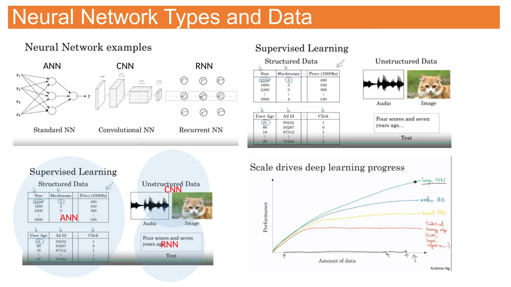
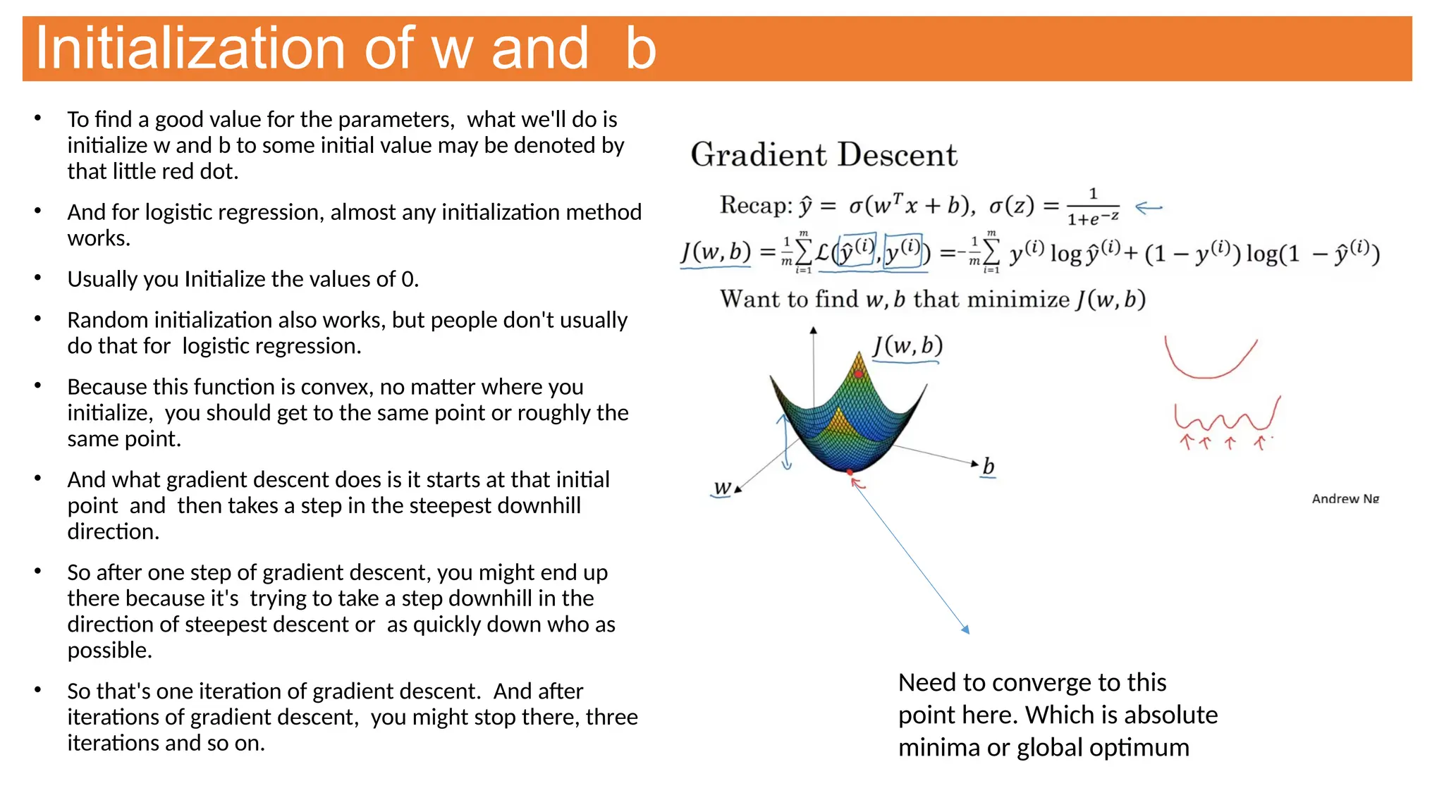
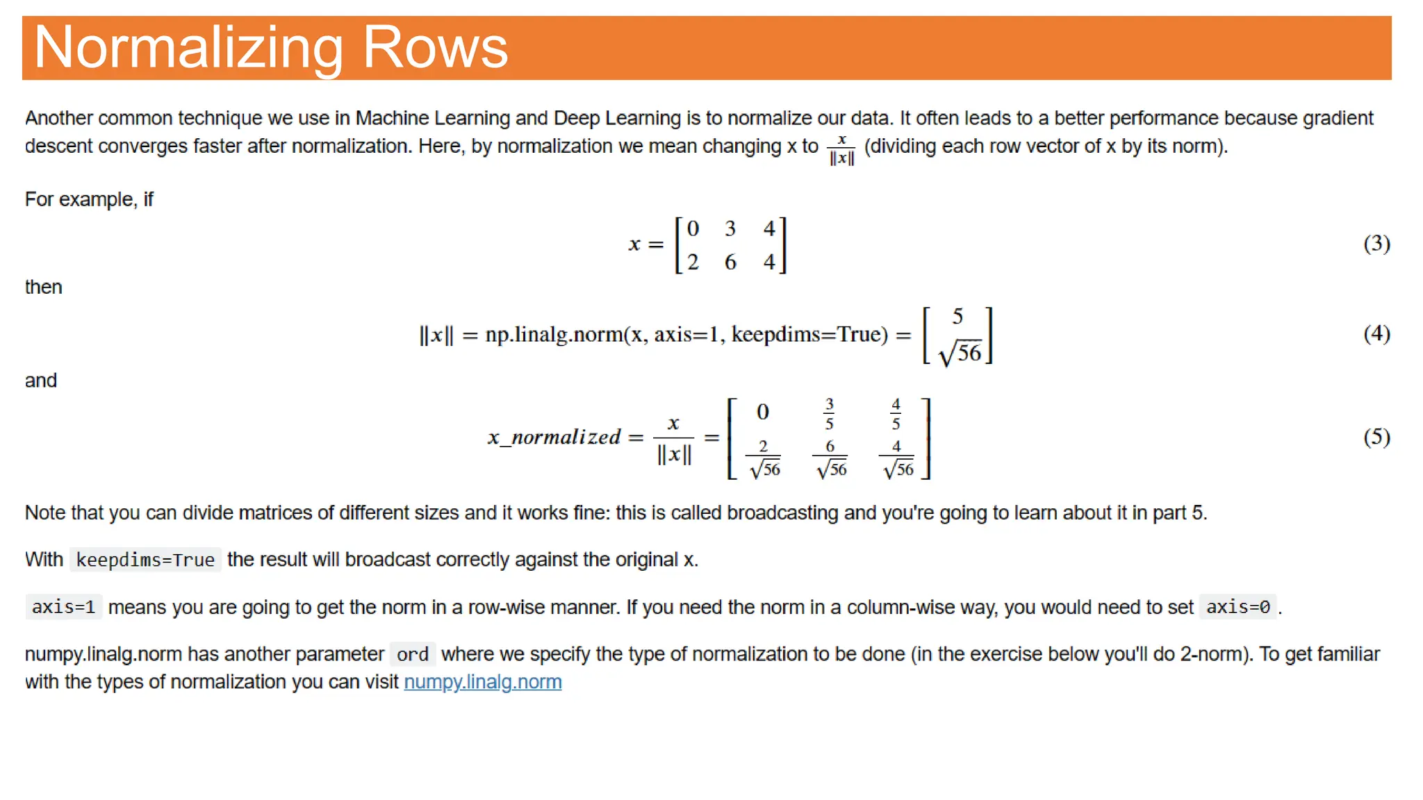
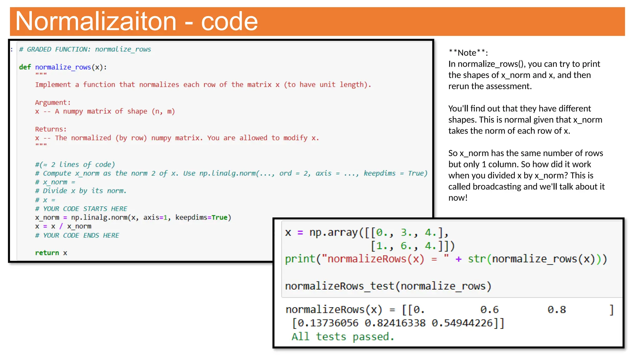
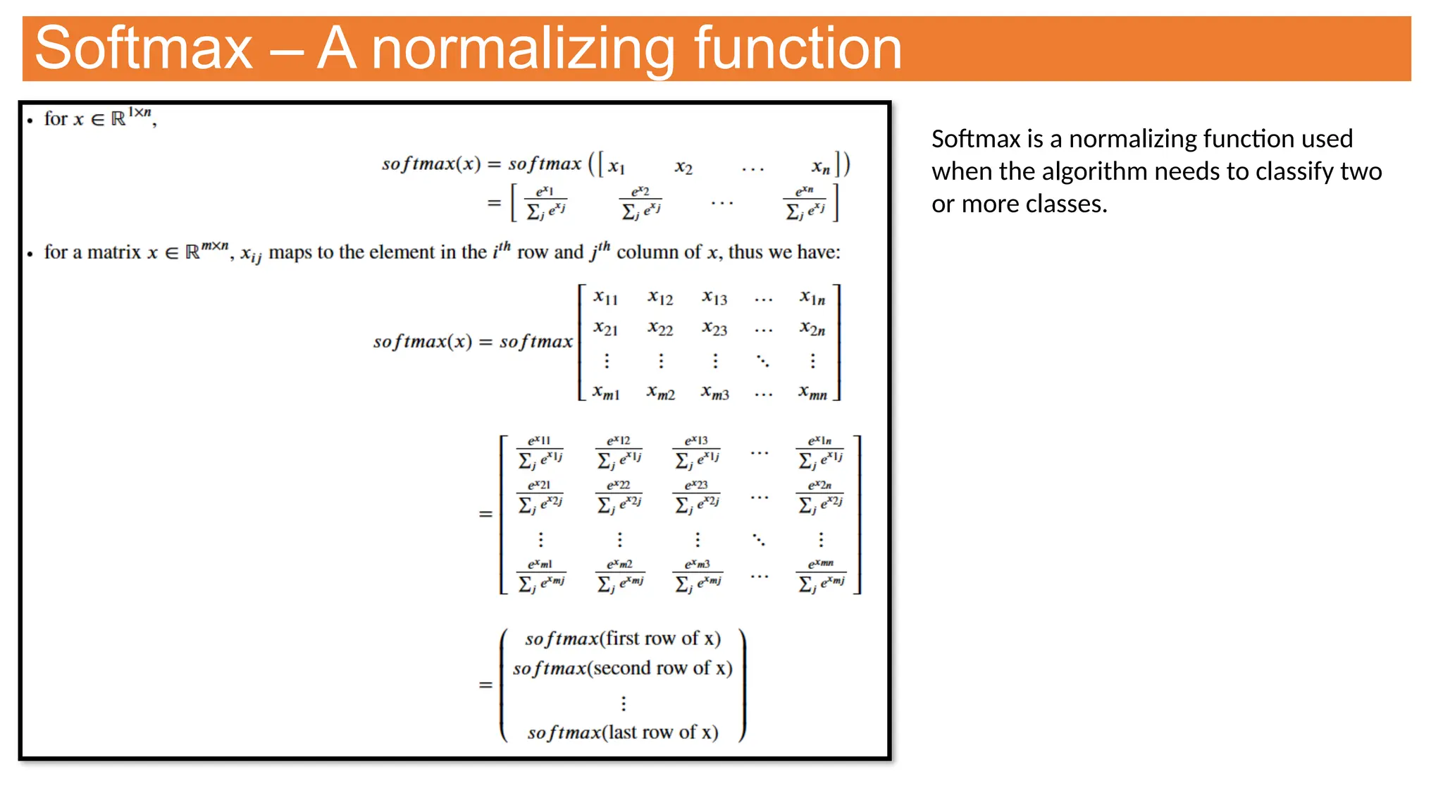
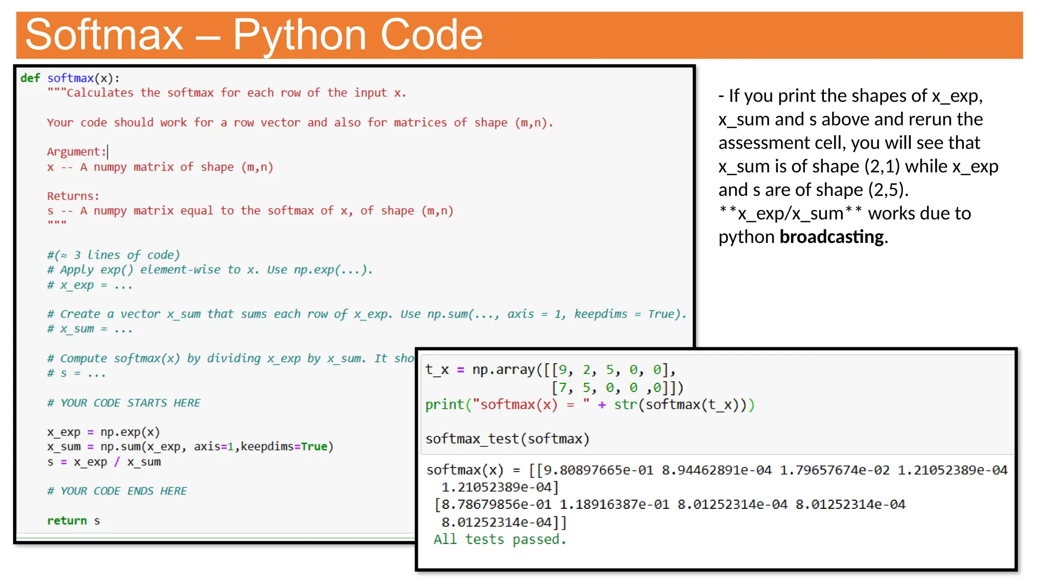
This document provides an overview of Convolutional Neural Networks (CNNs), detailing their architecture, parameters, and components like convolution, pooling, and fully connected layers. It discusses the importance of backpropagation, learnable parameters, and the benefits and drawbacks of pooling, as well as various types of pooling like max-pooling and average-pooling. The text also touches on object detection methods, including single-shot and two-shot detection, and key metrics for evaluating model performance like Intersection over Union (IoU) and Average Precision (AP).
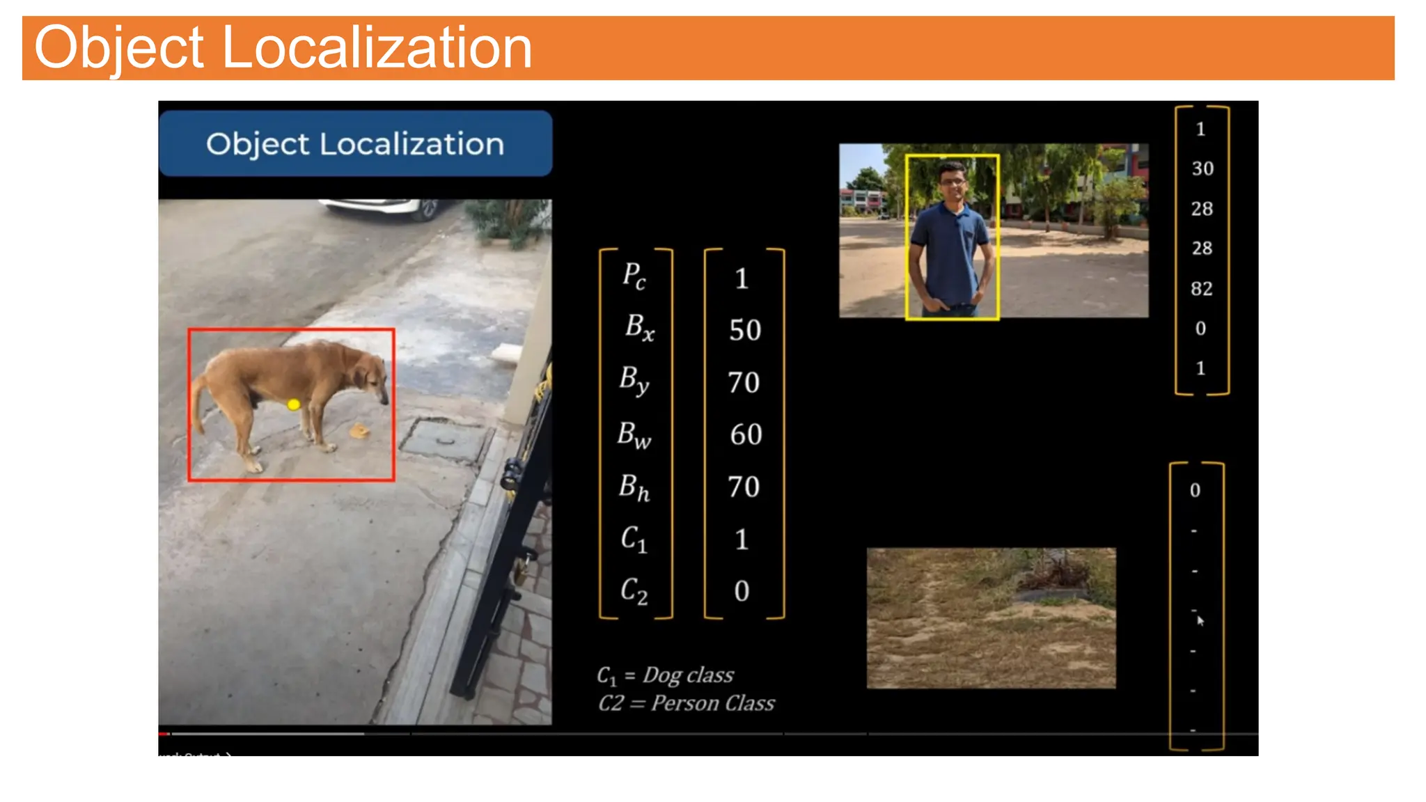
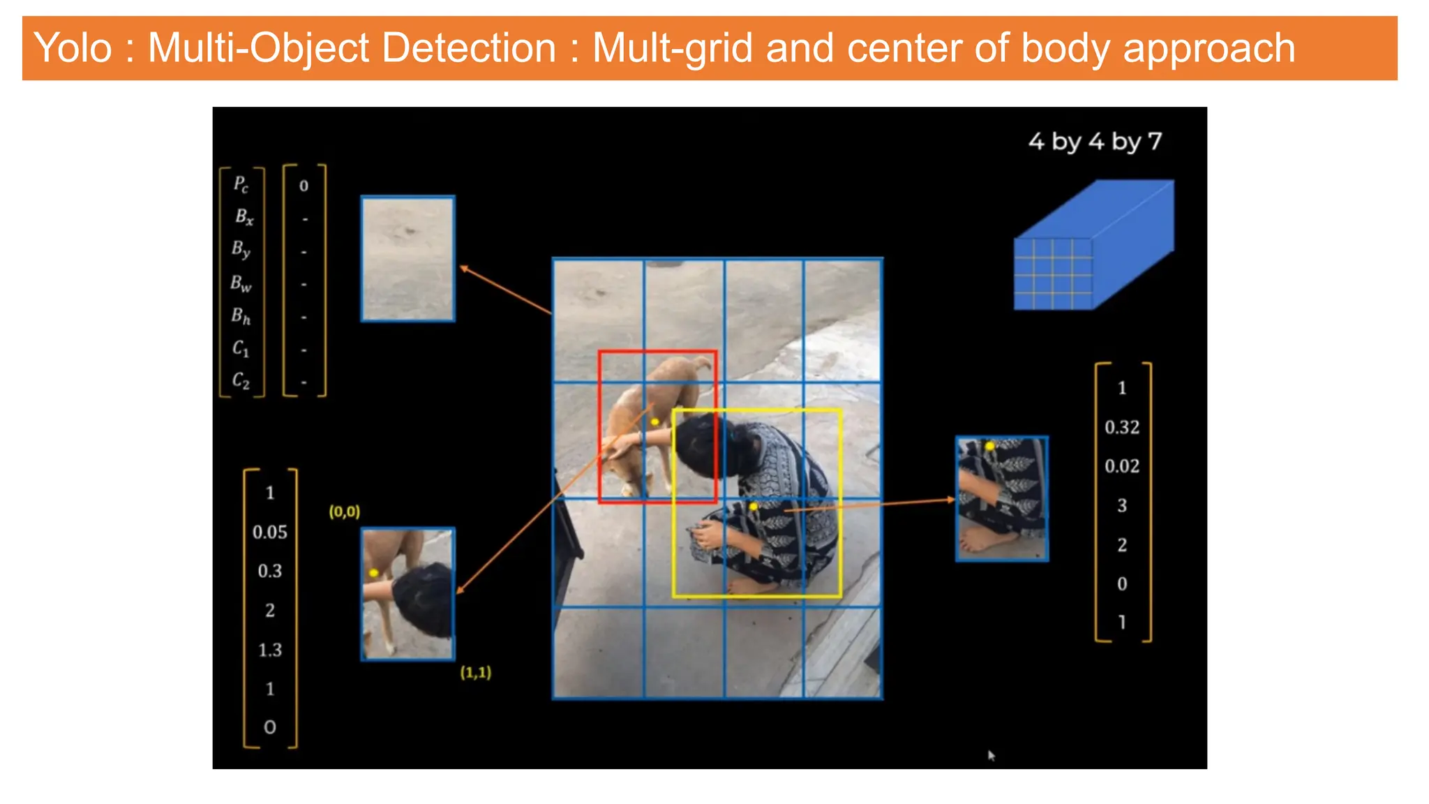
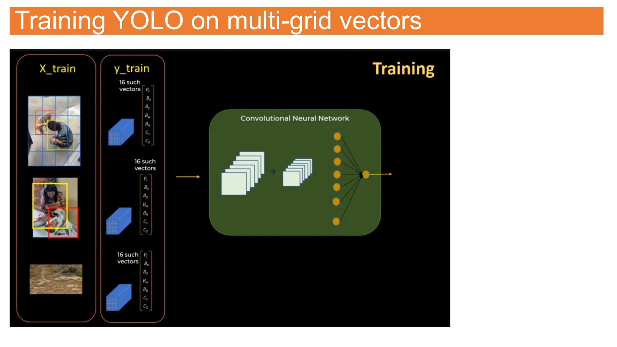
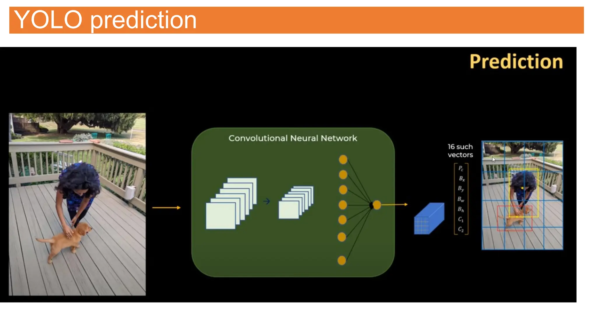
![YOLO Algorithm / Architecture
YOLO Algorithm for Object Detection Explained [+Examples] (v7labs.com)](https://image.slidesharecdn.com/selflearningdl-241015151050-eb475ec6/75/Deep-learning-requirement-and-notes-for-novoice-39-2048.jpg)
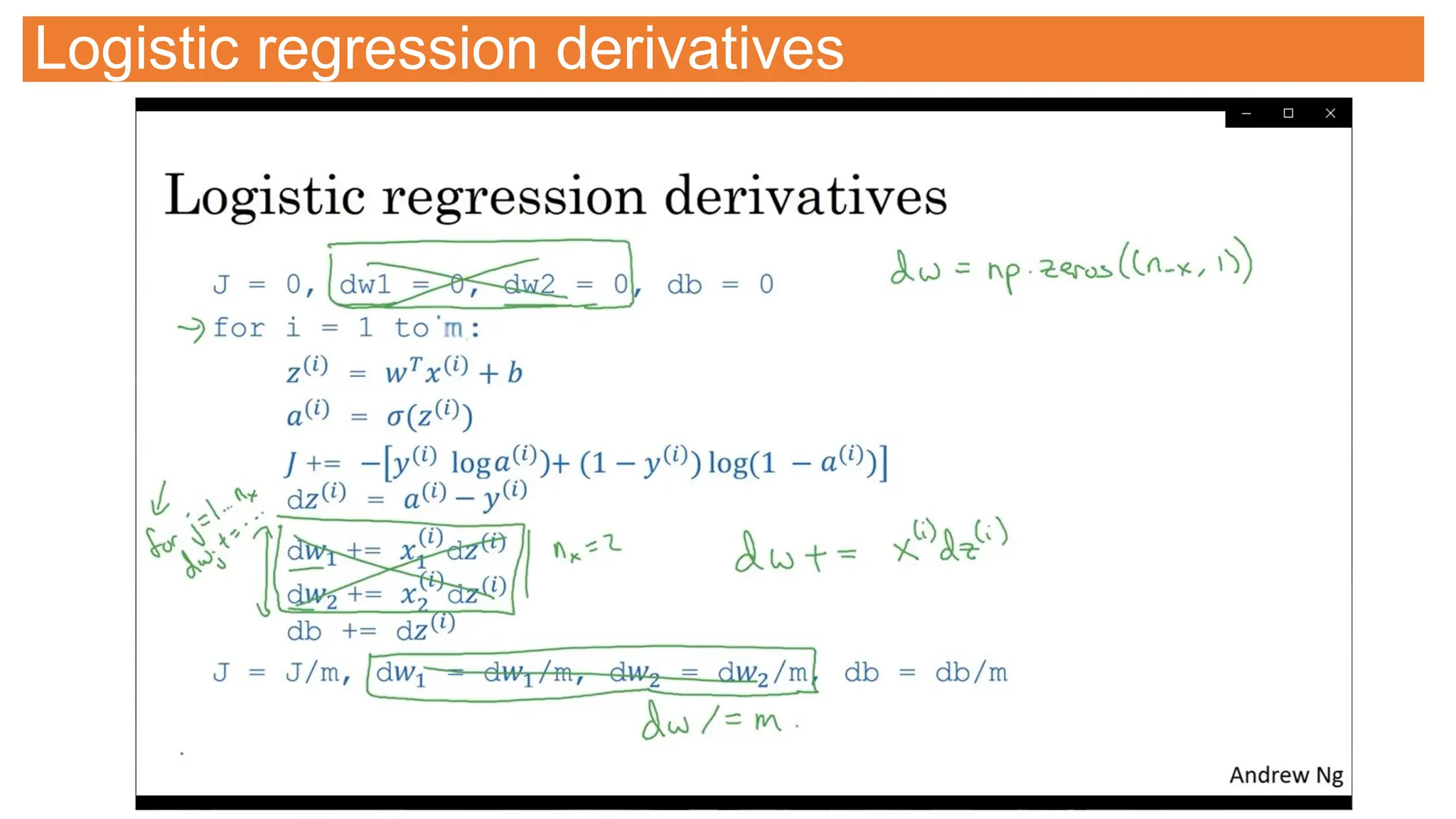
![Computing for entire dataset [m samples]
Major
for
loop
for
m
samples
Minor
for
loop
(required)
for
wn
weights
We need vectorization to get rid of
these for loop and write efficient code.
Necessary when m is very large.](https://image.slidesharecdn.com/selflearningdl-241015151050-eb475ec6/75/Deep-learning-requirement-and-notes-for-novoice-68-2048.jpg)
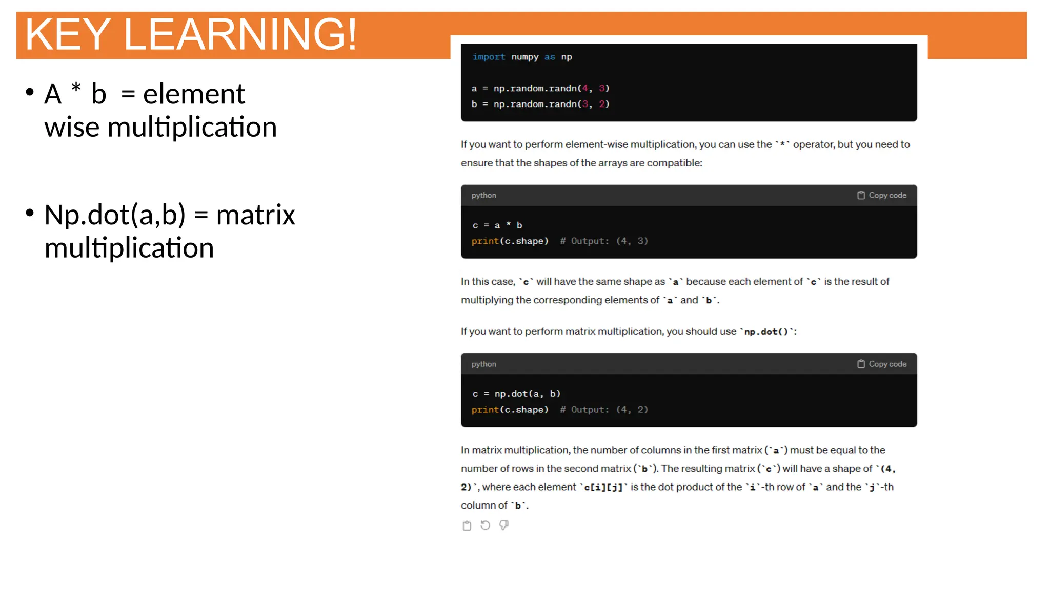
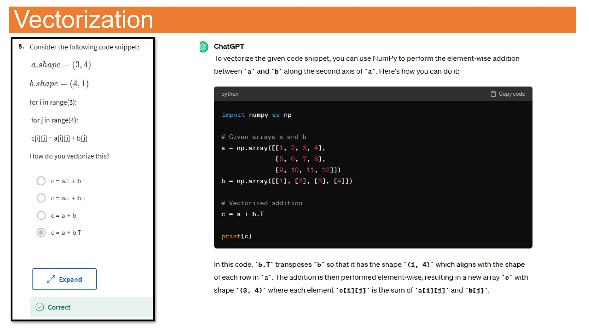
![What is Vectorization?
GPU and CPU can exceute parallel instructions
If you use built in function such as np.dot which don’t require
explicitly implementing for loop, it enables numpy to exploit
parallelism and thus your computation runs faster
Vectorization can significantly improve your code.
# Program to demonstrate how vectorization improves computational performance
# by comparing a vector dot product (parall implementation) vs foor loop implementation (sequential
execution)
# Ammar Ahmed
import time
import numpy as np
# Getting details about underlying hardware # running on google collab
import platform
print("Machine :" + str(platform.machine()))
print("Platform version :" + str(platform.version()))
print("Platform :" + str(platform.platform()))
# Generating array of elements
a = np.random.rand(1000000)
b = np.random.rand(1000000)
# Vector implementation
result=0
tic = time.time()
result = np.dot(a,b)
toc = time.time()
t1 = (toc - tic)*1000
print("Execution time of vectorized version = " + str(t1) + "ms " + " Computed Value :" + str(result))
# Non vector / loop implementation
result=0
tic = time.time()
for i in range(1000000):
result += a[i]*b[i]
toc = time.time()
t2 = (toc - tic)*1000
print("Execution time of sequential loop version = " + str(t2) + "ms "+ " Computed Value :" + str(result))
print("Time difference = " + str(t2-21) + "ms")](https://image.slidesharecdn.com/selflearningdl-241015151050-eb475ec6/75/Deep-learning-requirement-and-notes-for-novoice-69-2048.jpg)


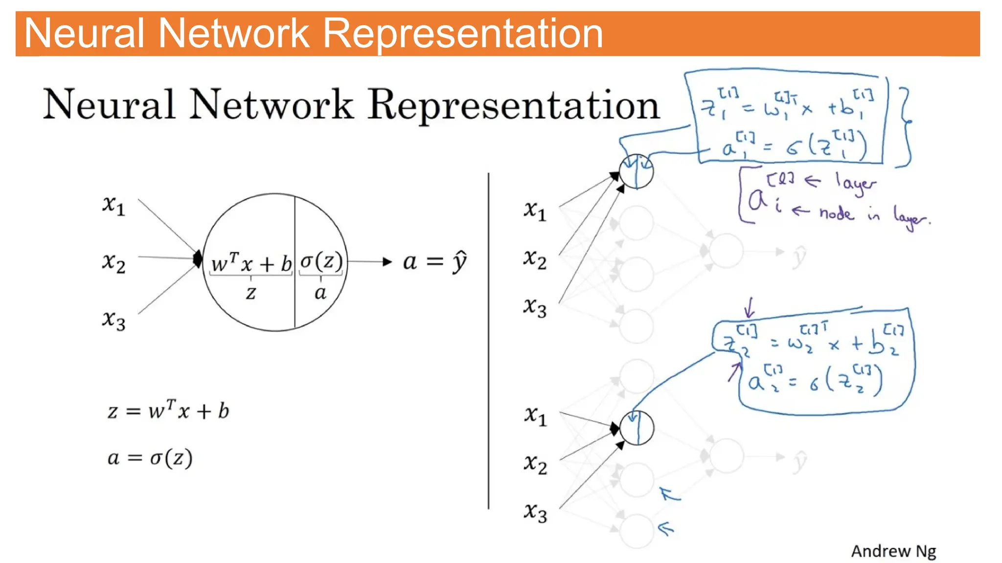
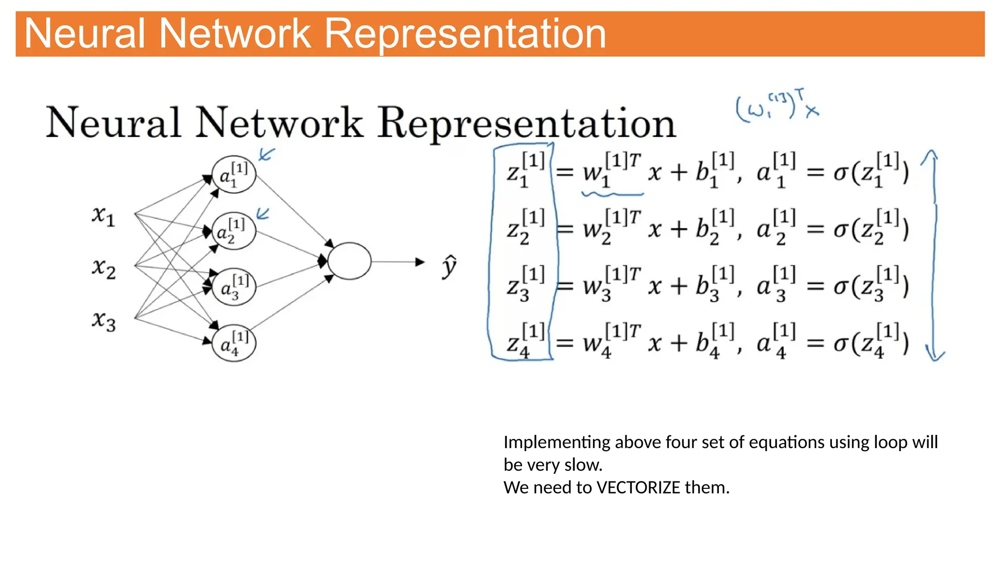
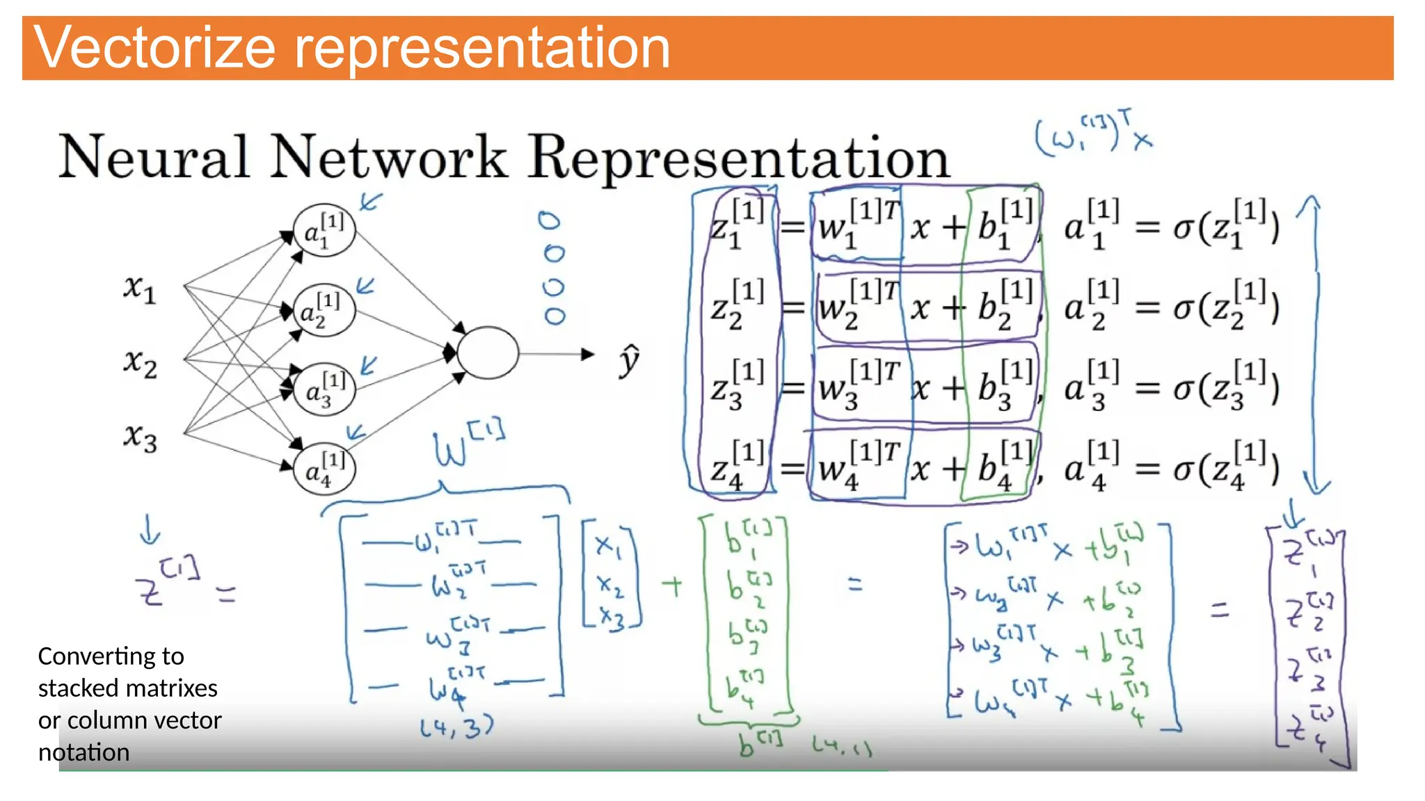
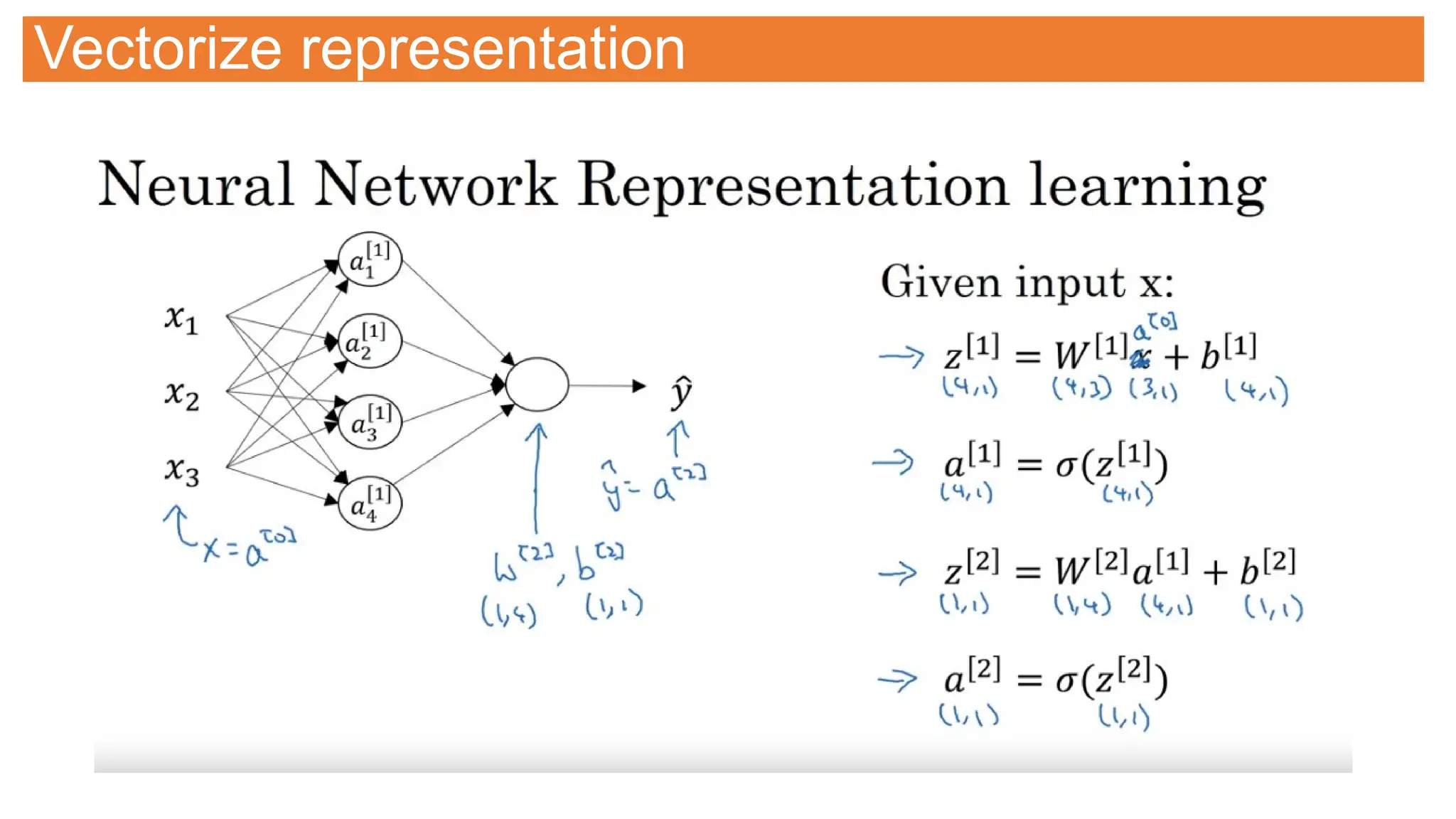
![Neural Network Representation
Two layer network
As we don’t count input
layer
[n] represent layer #
an represent node # in the
layer](https://image.slidesharecdn.com/selflearningdl-241015151050-eb475ec6/75/Deep-learning-requirement-and-notes-for-novoice-106-2048.jpg)