machine learning that uses artificial neural networks with multiple hidden layers to learn from vast amounts of data

1. Unit 2
CONVOLUTIONAL NEURAL NETWORKS

2. Convolution Neural Network
 Convolutional Neural Network (CNN) is the extended version of
artificial neural networks (ANN) which is predominantly used to extract
the feature from the grid-like matrix dataset. For example visual
datasets like images or videos where data patterns play an extensive
role.
 Around the 1980s, CNNs were developed and deployed for the first
time. A CNN could only detect handwritten digits at the time. CNN
was primarily used in various areas to read zip and pin codes etc.
 The most common aspect of any AI model is that it requires a massive
amount of data to train. This was one of the biggest problems that
CNN faced at the time, and due to this, they were only used in the
postal industry. Yann LeCun was the first to introduce convolutional
neural networks.

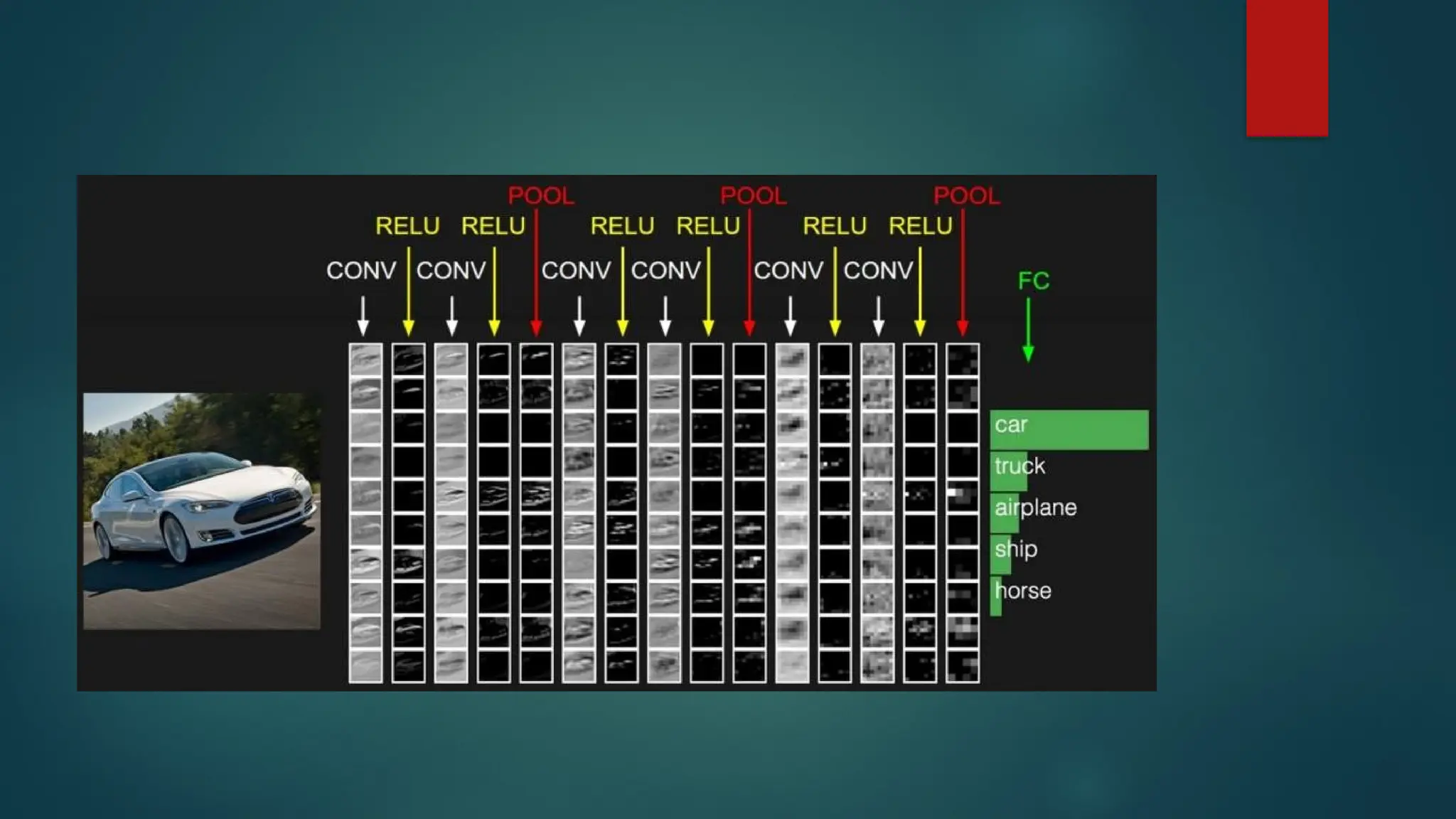
3.  Convolutional Neural Networks, commonly referred to as CNNs, are a
specialized kind of neural network architecture that is designed to
process data with a grid-like topology.
 CNNs are similar to other neural networks, but they have an added
layer of complexity due to the fact that they use a series of
convolutional layers.
 Convolutional layers perform a mathematical operation called
convolution, a sort of specialized matrix multiplication, on the input
data.
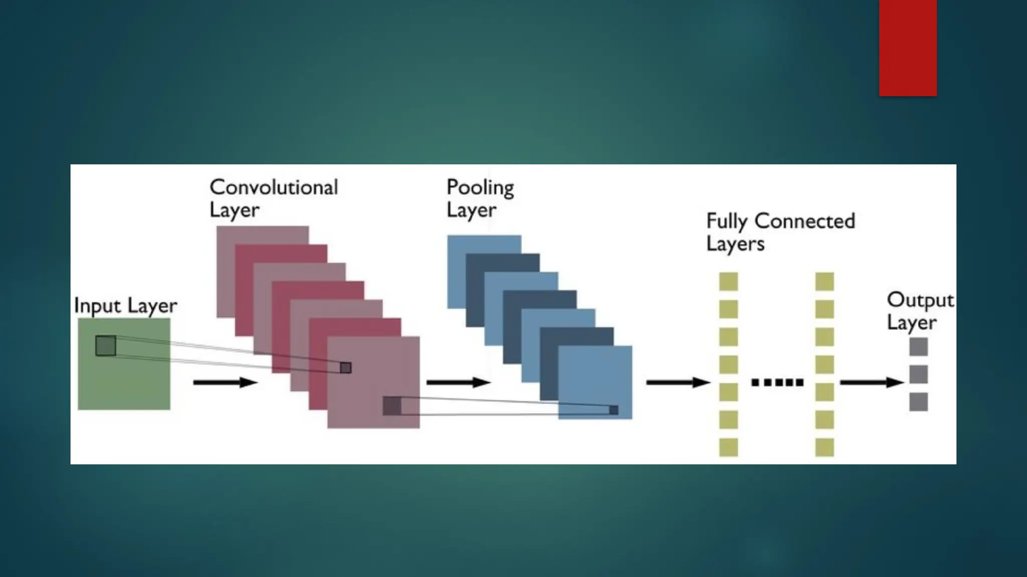
 The convolution operation helps to preserve the spatial relationship
between pixels by learning image features using small squares of
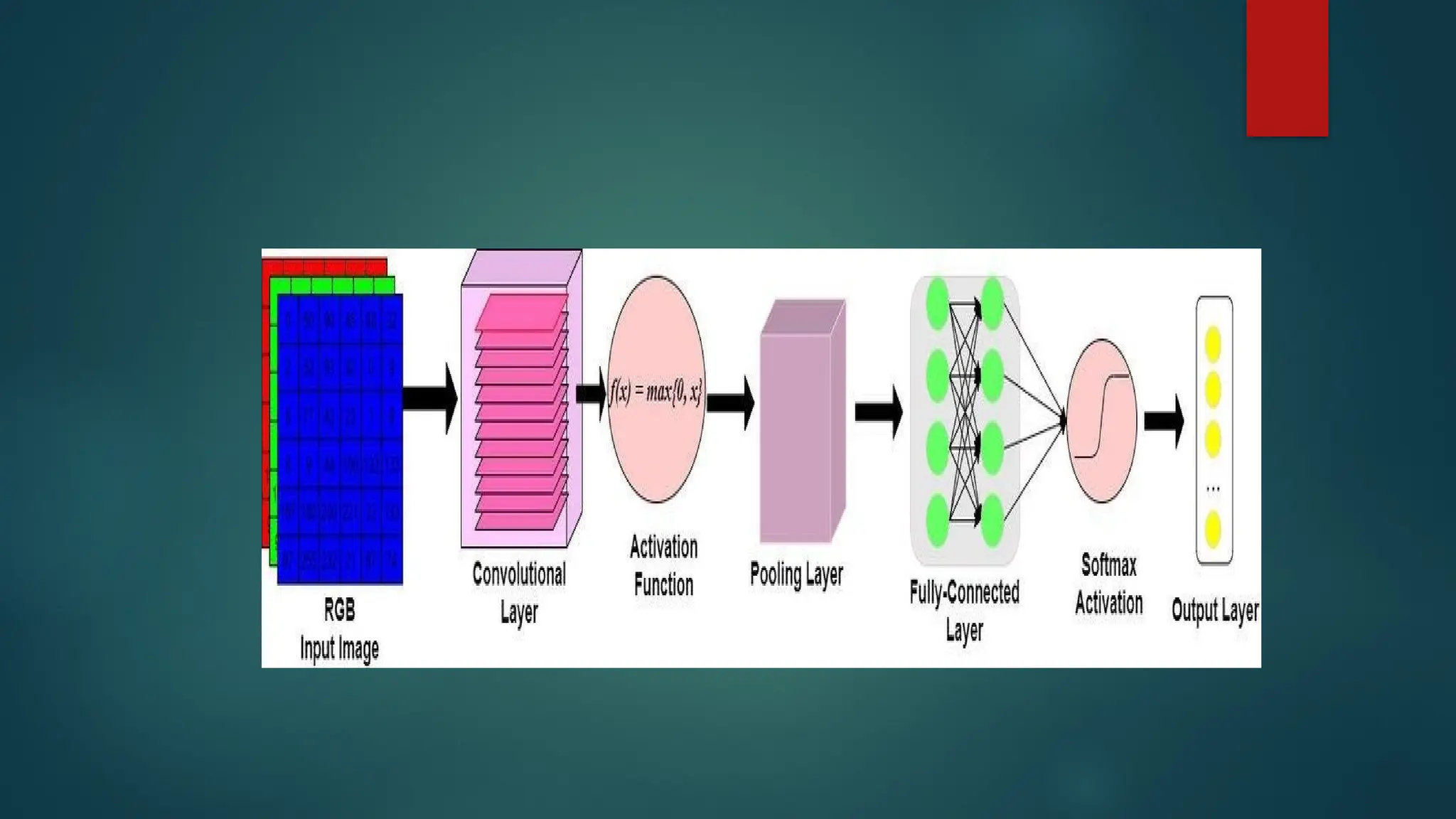
input data. . The picture below represents a typical CNN architecture.

5. Convolutional layers
 Convolutional layers operate by sliding a set of ‘filters’ or ‘kernels’ across the
input data.
 Each filter is designed to detect a specific feature or pattern, such as edges,
corners, or more complex shapes in the case of deeper layers.
 As these filters move across the image, they generate a map that signifies the
areas where those features were found. The output of the convolutional layer is a
feature map, which is a representation of the input image with the filters applied.
 Convolutional layers can be stacked to create more complex models, which
can learn more intricate features from images. Simply speaking, convolutional
layers are responsible for extracting features from the input images.
 These features might include edges, corners, textures, or more complex patterns.

6. Pooling layers
 Pooling layers follow the convolutional layers and are used to reduce the spatial
dimension of the input, making it easier to process and requiring less memory.
 In the context of images, “spatial dimensions” refer to the width and height of the
image.
 An image is made up of pixels, and you can think of it like a grid, with rows and
columns of tiny squares (pixels).
 By reducing the spatial dimensions, pooling layers help reduce the number of
parameters or weights in the network.
 This helps to combat over-fitting and help train the model in a fast manner.
 Max pooling helps in reducing computational complexity, owing to reduction in
size of feature map, and making the model invariant to small transitions. Without
max pooling, the network would not gain the ability to recognize features
irrespective of small shifts or rotations. This would make the model less robust to
variations in object positioning within the image, possibly affecting accuracy.

7.  There are two main types of pooling: max pooling and average
pooling. Max pooling takes the maximum value from each feature
map.
 For example, if the pooling window size is 2×2, it will pick the pixel
with the highest value in that 2×2 region.
 Max pooling effectively captures the most prominent feature or
characteristic within the pooling window. Average pooling
calculates the average of all values within the pooling window. It
provides a smooth, average feature representation.

8. Fully connected layers
 Fully-connected layers are one of the most basic types of layers in a
convolutional neural network (CNN). As the name suggests, each
neuron in a fully-connected layer is Fully connected- to every other
neuron in the previous layer.
 Fully connected layers are typically used towards the end of a CNN-
when the goal is to take the features learned by the convolutional
and max pooling layers and use them to make predictions such as
classifying the input to a label.
 For example, if we were using a CNN to classify images of animals,
the final Fully connected layer might take the features learned by
the previous layers and use them to classify an image as containing
a dog, cat, bird, etc.

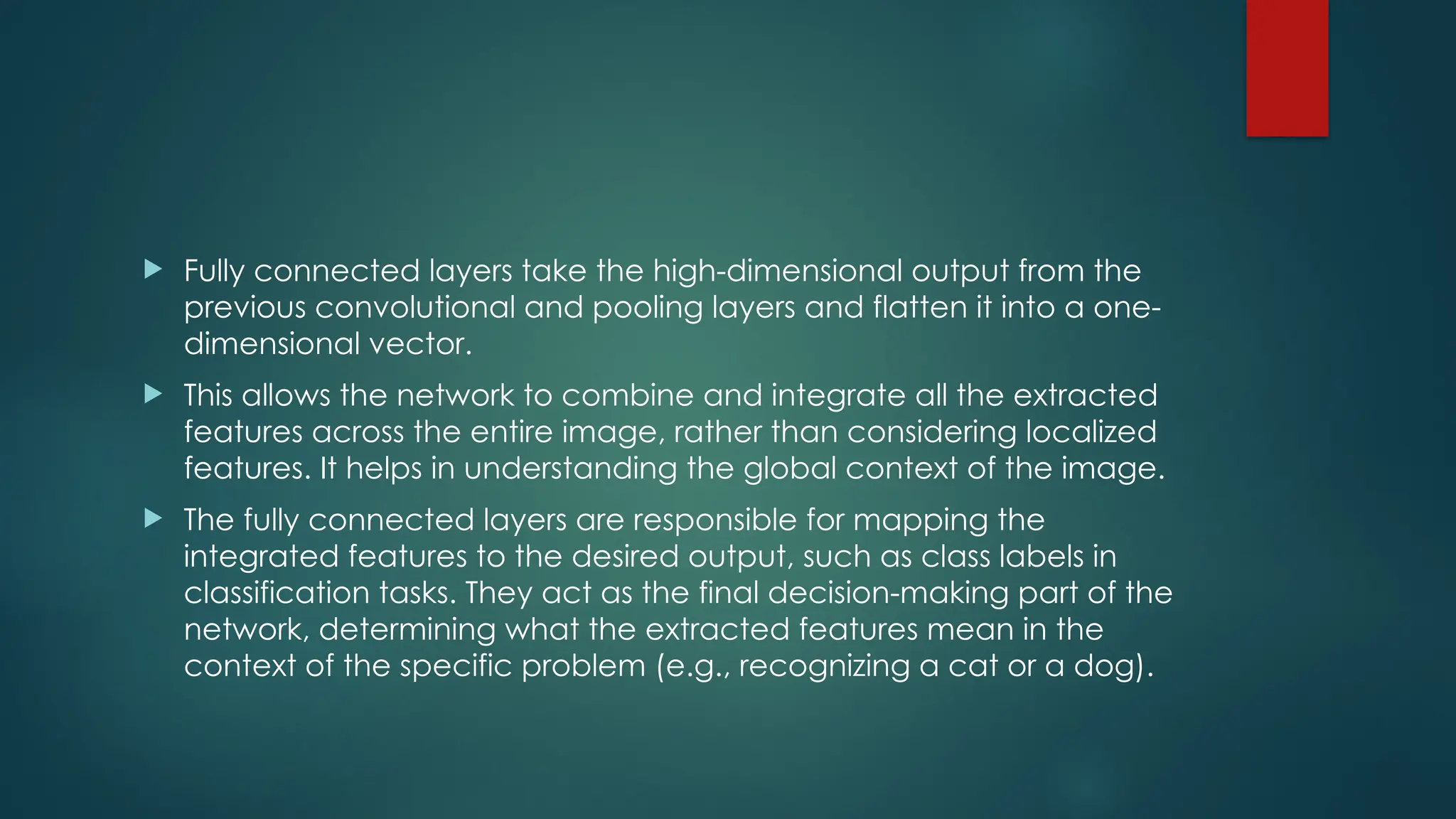
9.  Fully connected layers take the high-dimensional output from the
previous convolutional and pooling layers and flatten it into a one-
dimensional vector.
 This allows the network to combine and integrate all the extracted
features across the entire image, rather than considering localized
features. It helps in understanding the global context of the image.
 The fully connected layers are responsible for mapping the
integrated features to the desired output, such as class labels in
classification tasks. They act as the final decision-making part of the
network, determining what the extracted features mean in the
context of the specific problem (e.g., recognizing a cat or a dog).

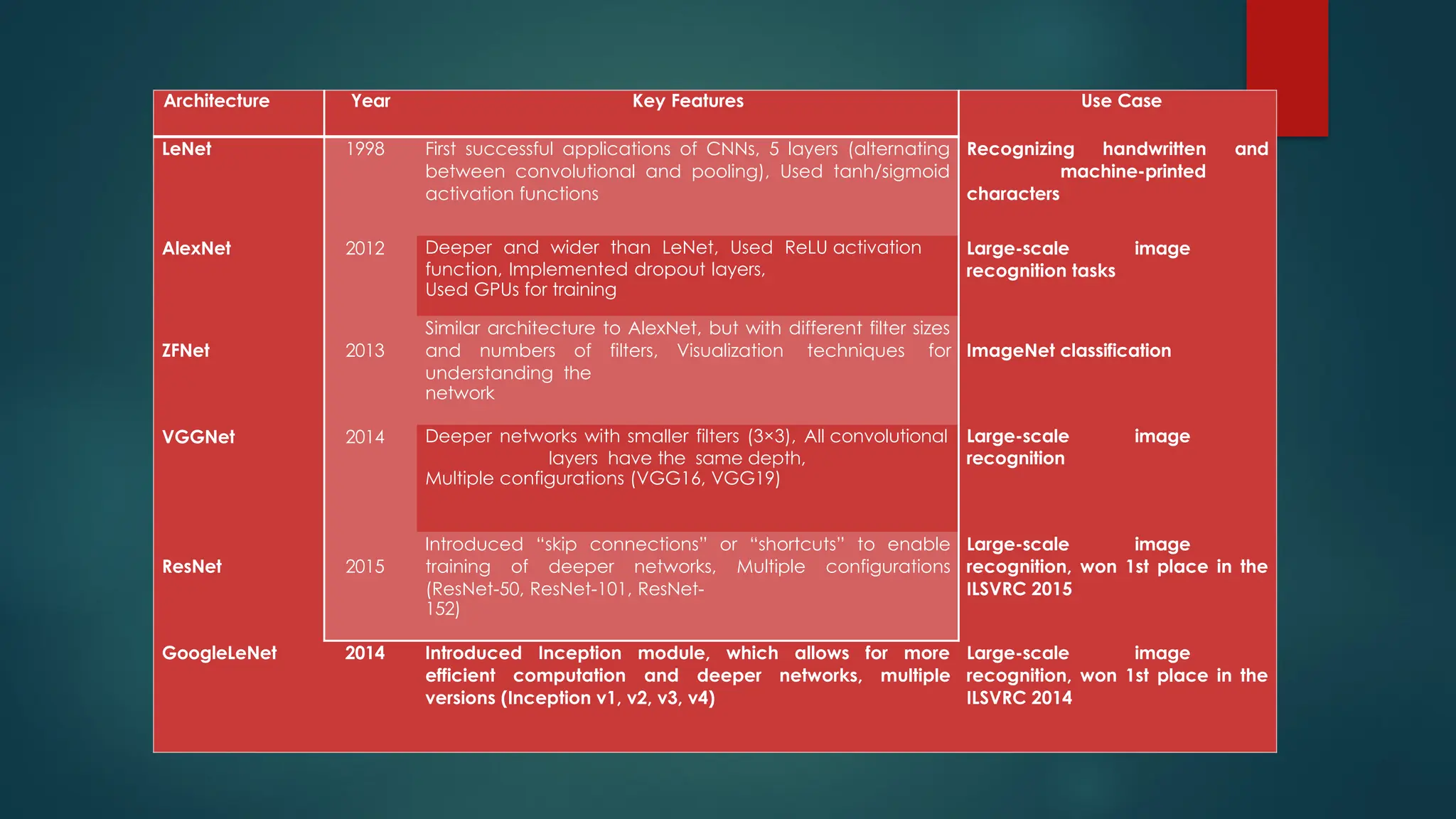
11. Architecture Year Key Features Use Case
LeNet 1998 First successful applications of CNNs, 5 layers (alternating
between convolutional and pooling), Used tanh/sigmoid
activation functions
Recognizing handwritten and
machine-printed
characters
AlexNet 2012 Deeper and wider than LeNet, Used ReLU activation
function, Implemented dropout layers,
Used GPUs for training
Large-scale image
recognition tasks
ZFNet 2013
Similar architecture to AlexNet, but with different filter sizes
and numbers of filters, Visualization techniques for
understanding the
network
ImageNet classification
VGGNet 2014 Deeper networks with smaller filters (3×3), All convolutional
layers have the same depth,
Multiple configurations (VGG16, VGG19)
Large-scale image
recognition
ResNet 2015
Introduced “skip connections” or “shortcuts” to enable
training of deeper networks, Multiple configurations
(ResNet-50, ResNet-101, ResNet-
152)
Large-scale image
recognition, won 1st place in the
ILSVRC 2015
GoogleLeNet 2014 Introduced Inception module, which allows for more
efficient computation and deeper networks, multiple
versions (Inception v1, v2, v3, v4)
Large-scale image
recognition, won 1st place in the
ILSVRC 2014

12. Activation Layer:
 Activation Layer: By adding an activation function to the output of
the preceding layer, activation layers add nonlinearity to the
network. it will apply an element-wise activation function to the
output of the convolution layer. Some common activation functions
are RELU, Tanh, Leaky RELU, etc. The volume remains unchanged
hence output volume will have dimensions 32 x 32 x 12.
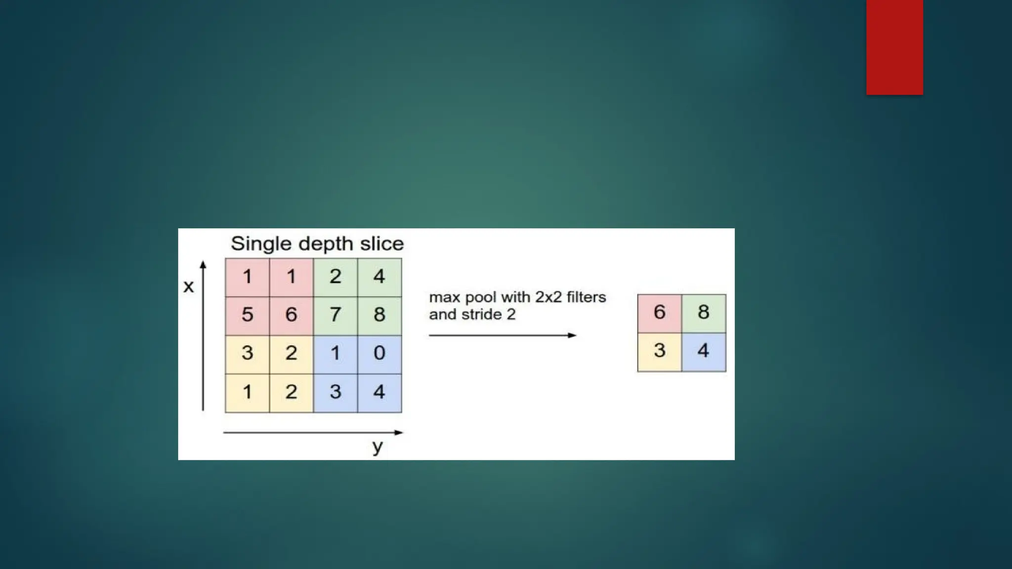
 Pooling layer: This layer is periodically inserted in the convnets and
its main function is to reduce the size of volume which makes the
computation fast reduces memory and also prevents over- fitting.
Two common types of pooling layers are max pooling and average
pooling. If we use a max pool with 2 x 2 filters and stride 2, the
resultant volume will be of dimension 16x16x12.

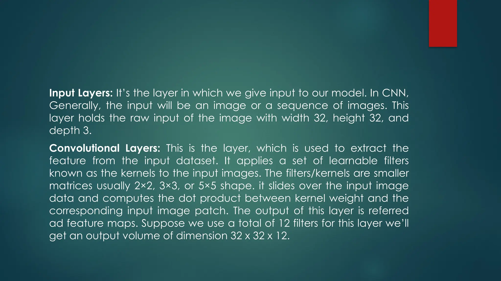
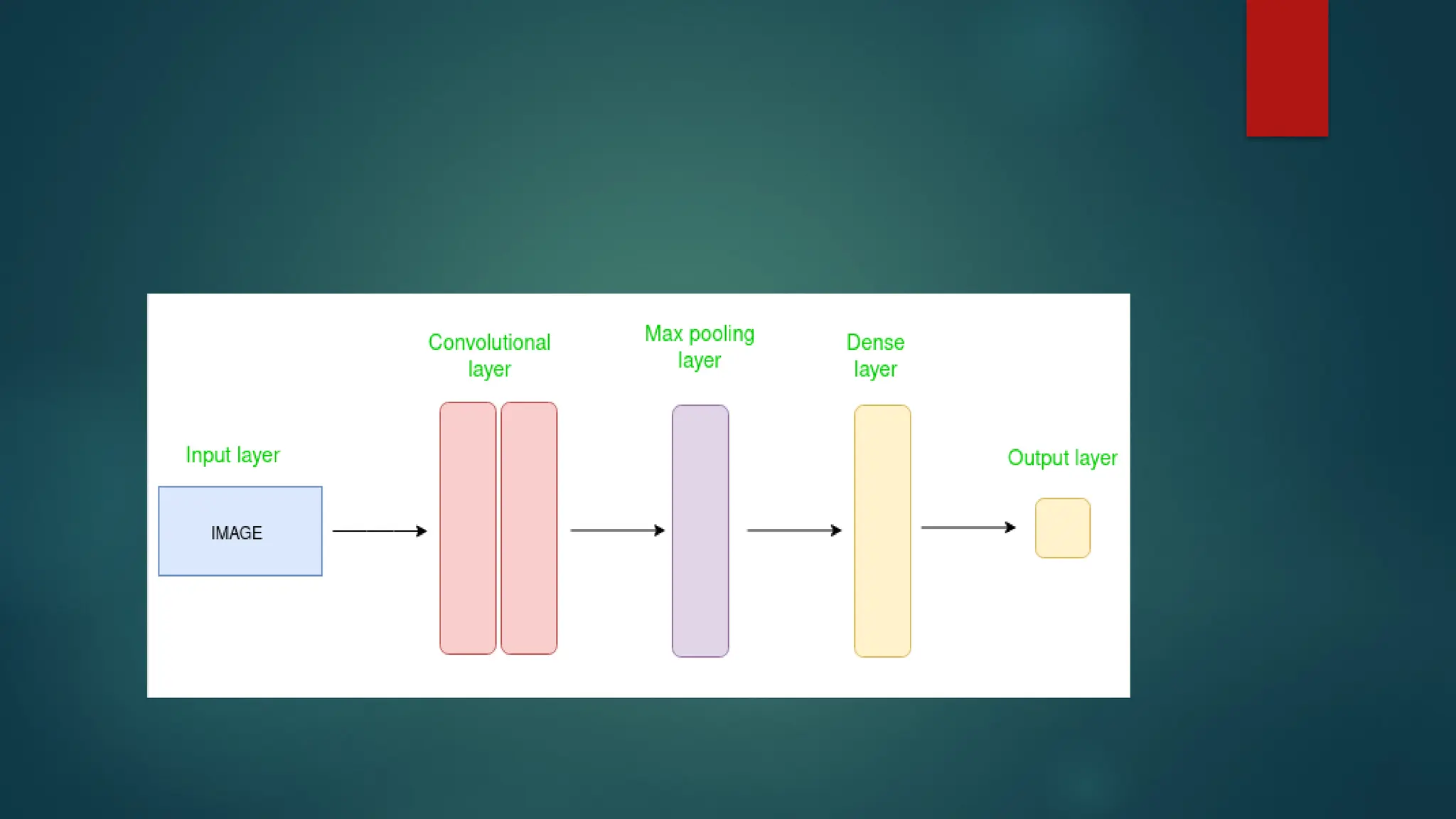
13. Input Layers: It’s the layer in which we give input to our model. In CNN,
Generally, the input will be an image or a sequence of images. This
layer holds the raw input of the image with width 32, height 32, and
depth 3.
Convolutional Layers: This is the layer, which is used to extract the
feature from the input dataset. It applies a set of learnable filters
known as the kernels to the input images. The filters/kernels are smaller
matrices usually 2×2, 3×3, or 5×5 shape. it slides over the input image
data and computes the dot product between kernel weight and the
corresponding input image patch. The output of this layer is referred
ad feature maps. Suppose we use a total of 12 filters for this layer we’ll
get an output volume of dimension 32 x 32 x 12.

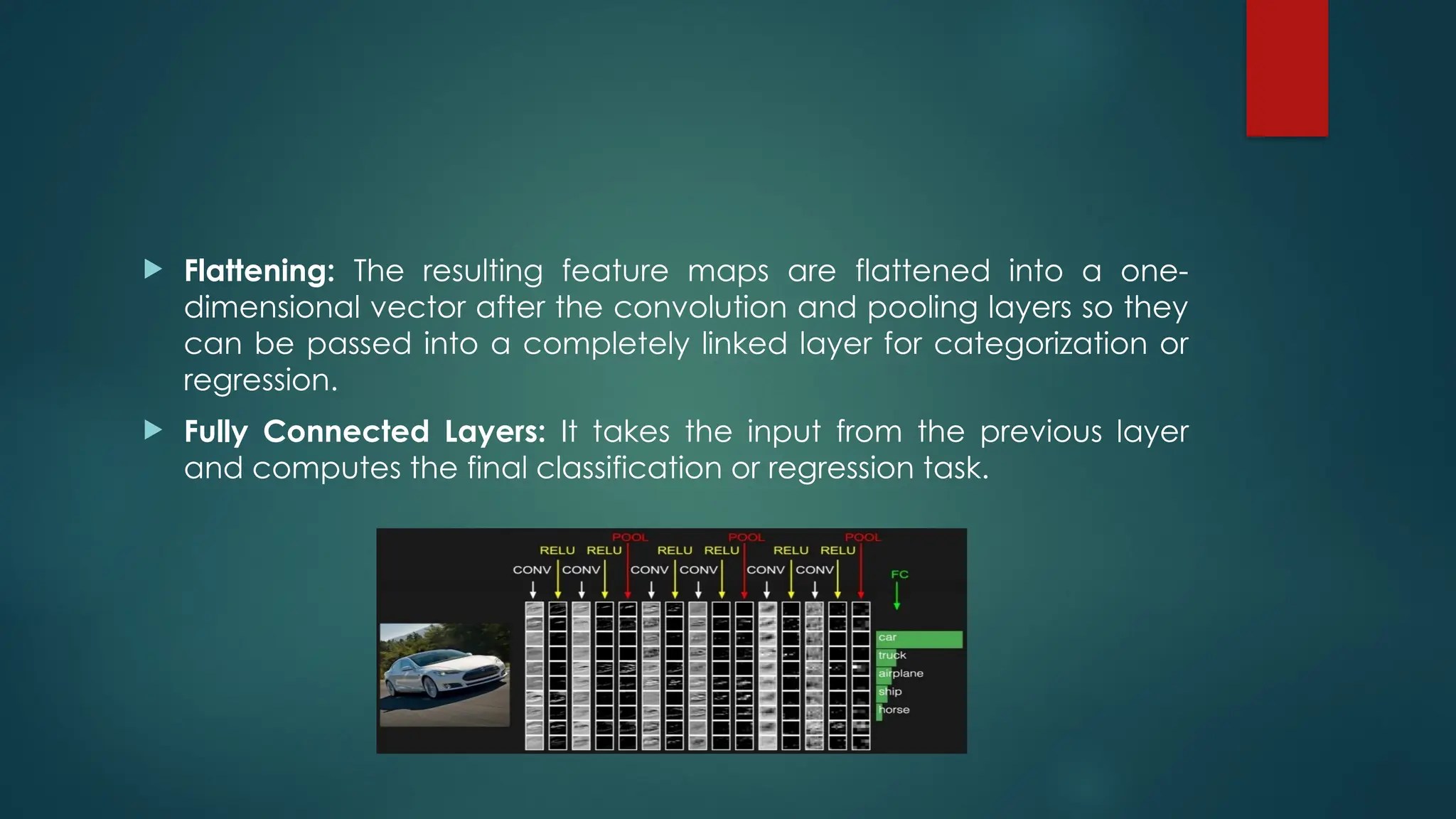
14.  Flattening: The resulting feature maps are flattened into a one-
dimensional vector after the convolution and pooling layers so they
can be passed into a completely linked layer for categorization or
regression.
 Fully Connected Layers: It takes the input from the previous layer
and computes the final classification or regression task.

16.  Output Layer: The output from the fully connected layers is then fed
into a logistic function for classification tasks like sigmoid or softmax
which converts the output of each class into the probability score of
each class

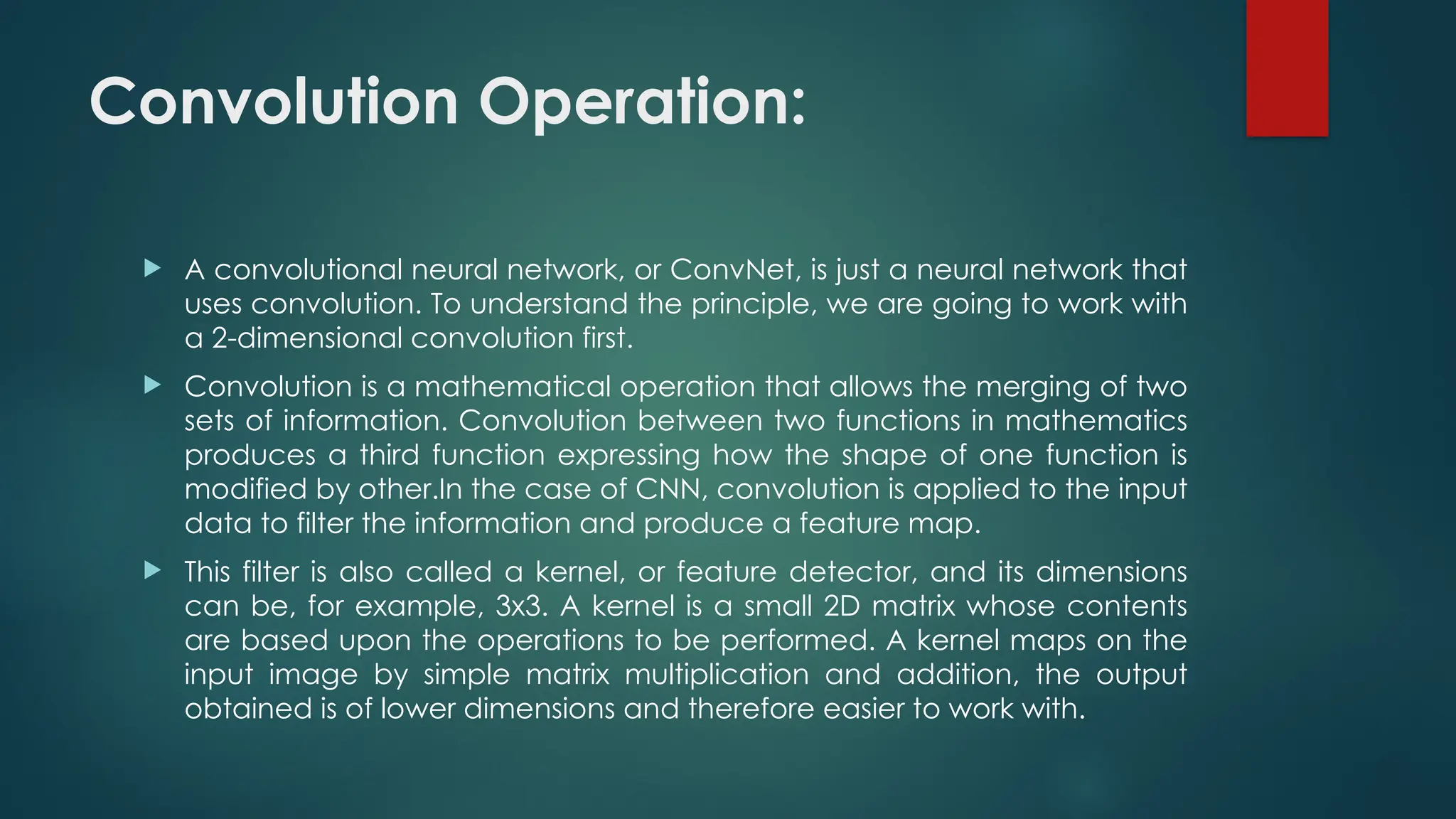
17. Convolution Operation:
 A convolutional neural network, or ConvNet, is just a neural network that
uses convolution. To understand the principle, we are going to work with
a 2-dimensional convolution first.
 Convolution is a mathematical operation that allows the merging of two
sets of information. Convolution between two functions in mathematics
produces a third function expressing how the shape of one function is
modified by other.In the case of CNN, convolution is applied to the input
data to filter the information and produce a feature map.
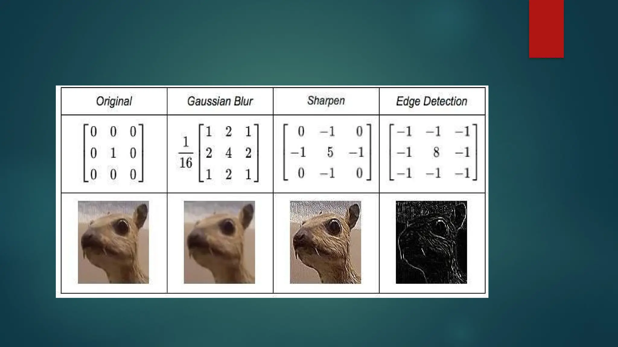
 This filter is also called a kernel, or feature detector, and its dimensions
can be, for example, 3x3. A kernel is a small 2D matrix whose contents
are based upon the operations to be performed. A kernel maps on the
input image by simple matrix multiplication and addition, the output
obtained is of lower dimensions and therefore easier to work with.

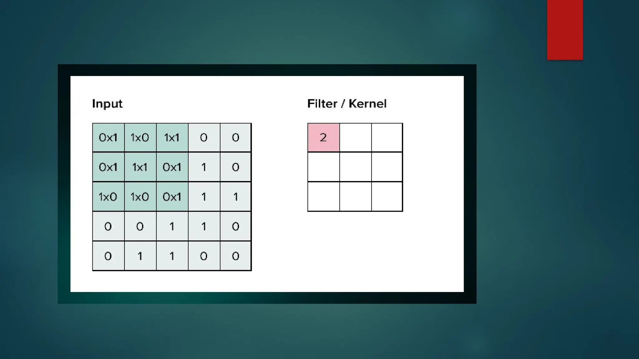
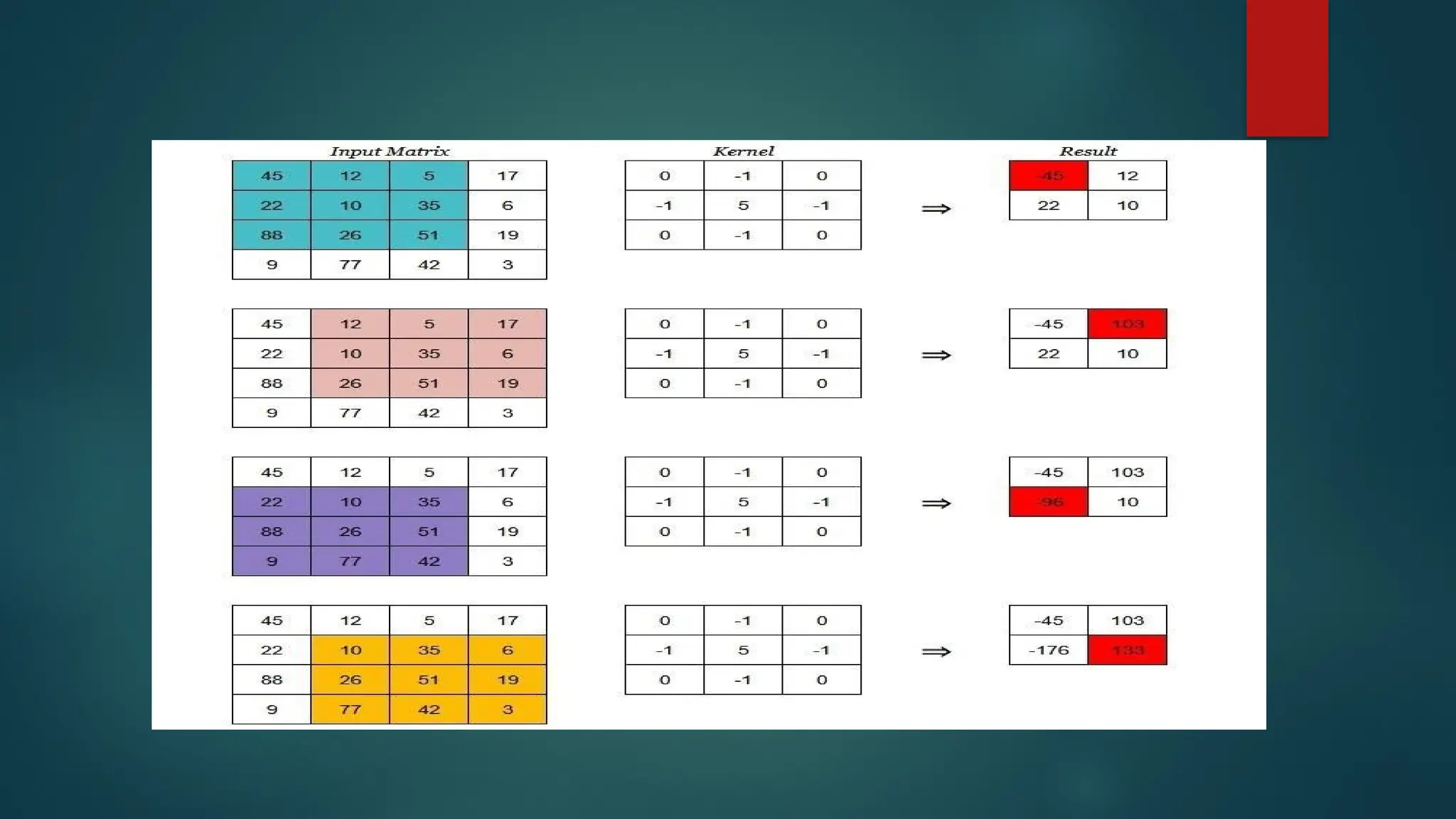
22.  The kernel gets into position at the top-left corner of the input matrix.
 Then it starts moving left to right, calculating the dot product and
saving it to a new matrix until it has reached the last column.
 Next, kernel resets its position at first column but now it slides one row
to the bottom. Thus following the fashion left-right and top-bottom.
 Steps 2 and 3are repeated till the entire input has been processed.
 For a 3D input matrix the movement of the kernel will be from front
to back, left to right and top to bottom.

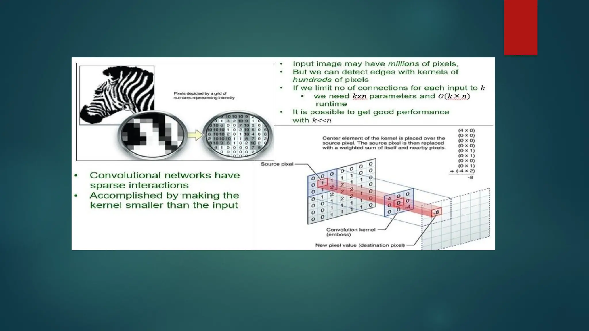
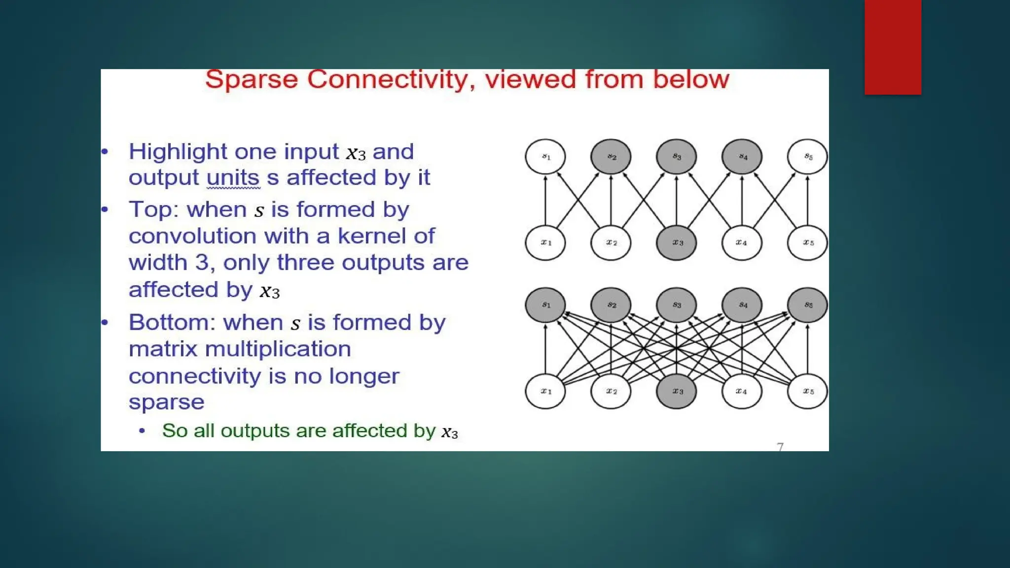
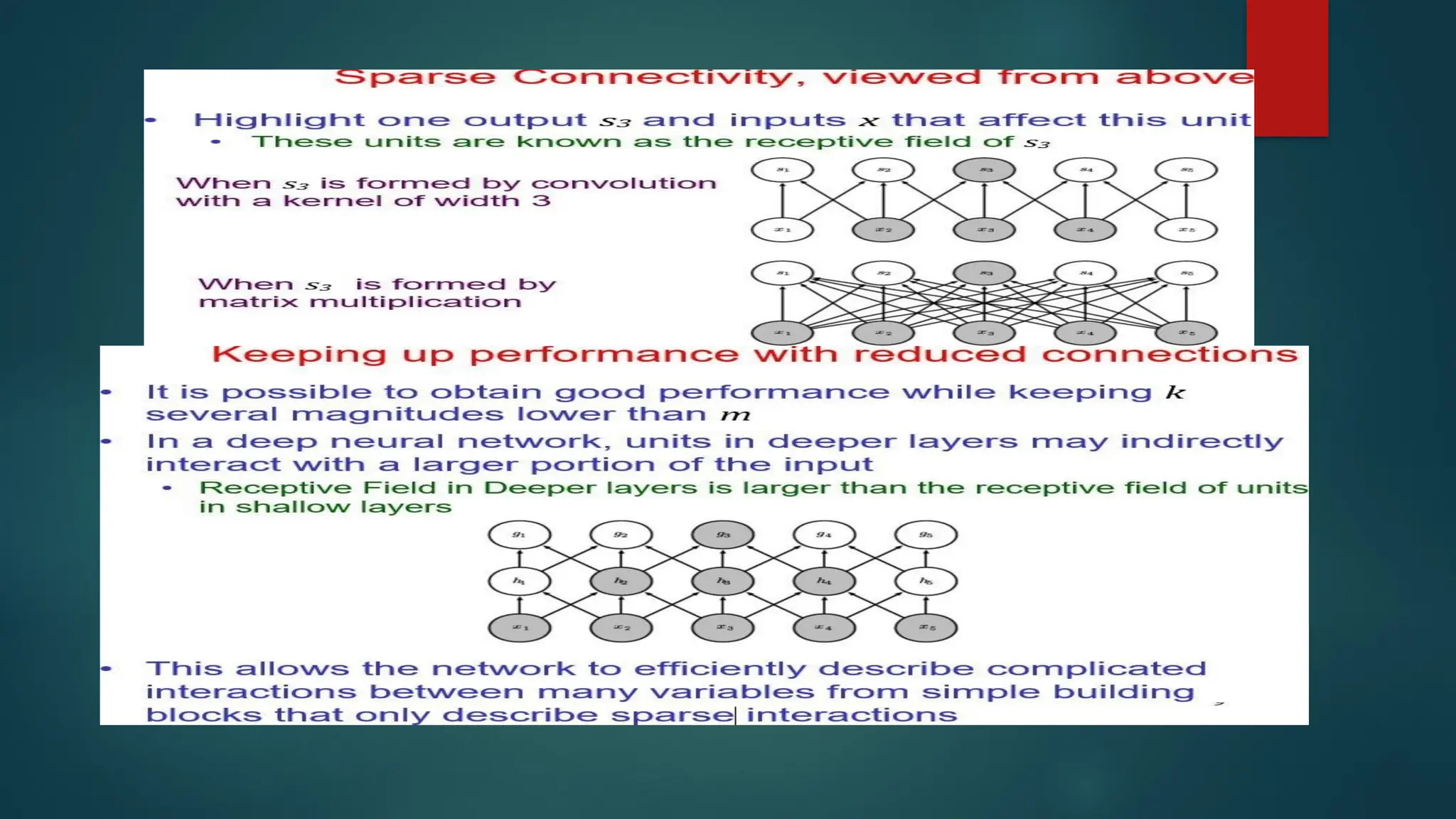
23. Sparse Interactions (Connectivity)
 A Convolution layer defines a window or filter or kernel by which
they examine a subset of the data, and subsequently scans the
data looking through this window.
 We can parameterize the window to look for specific features (e.g.
edges within an image). The output they produce focuses solely on
the regions of the data which exhibited the feature it was searching
for.
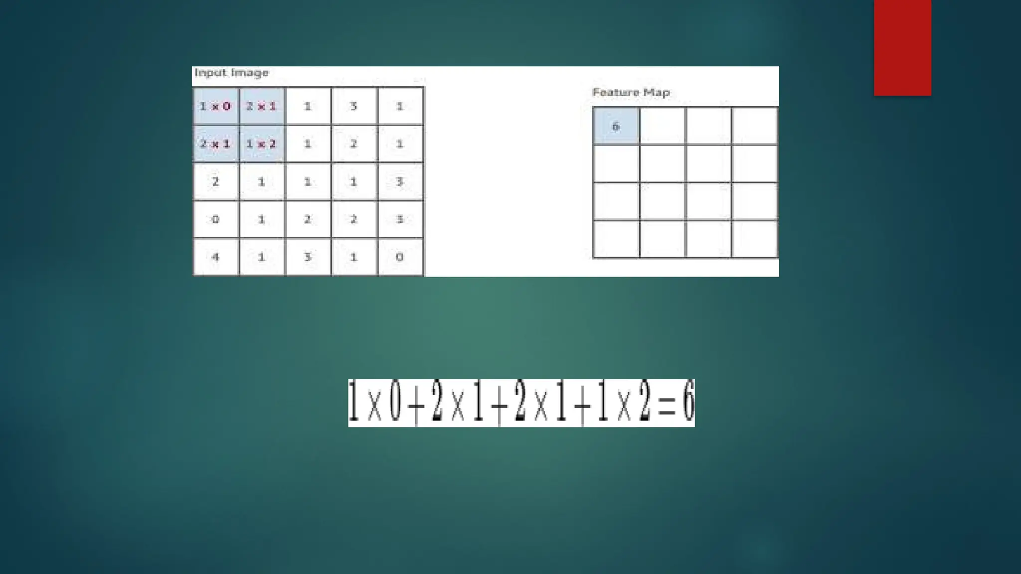
 This is what we call sparse connectivity or sparse interactions or
sparse weights. Actually it limits the activated connections at each
layer. In the example below an 5x5 input with a 2x2 filter produces a
reduced 4x4 output.

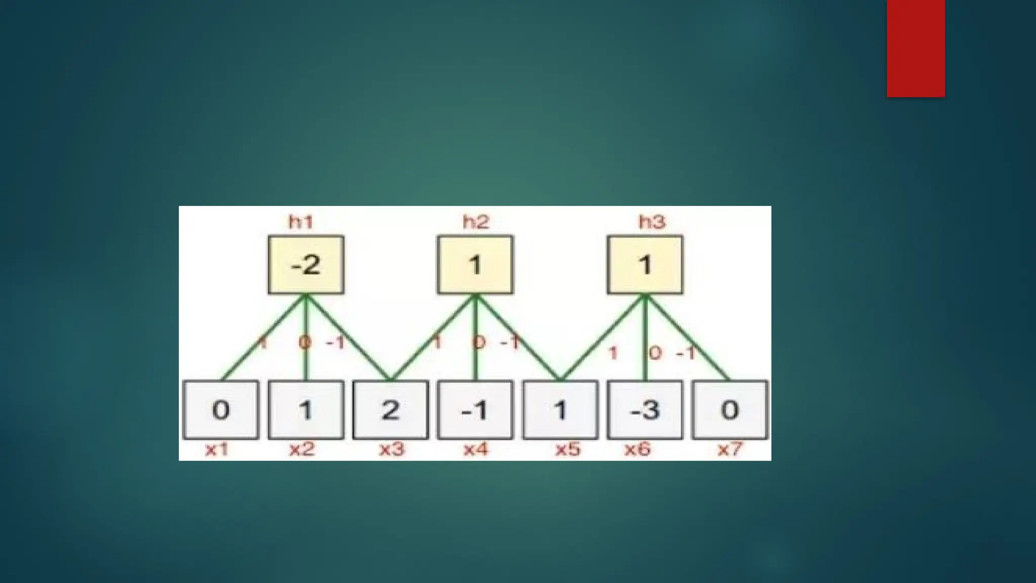
28. Parameter (Weight) Sharing
If computing one feature at a spatial point (x1, y1) is useful then it should also be
useful at some other spatial point say (x2, y2). It means that for a single two-
dimensional slice i.e., for creating one activation map, neurons are constrained to
use the same set of weights.
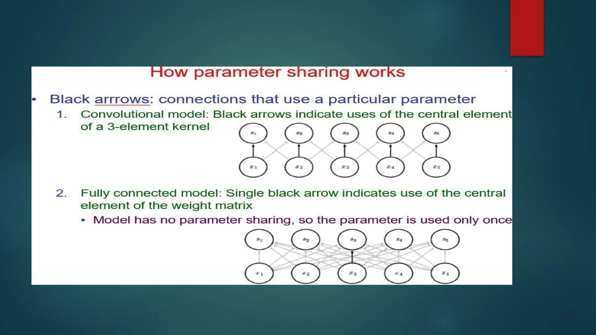
In a traditional neural network, each element of the weight matrix is used once
and then never revisited, while convolution network has shared parameters i.e., for
getting output, weights applied to one input are the same as the weight applied
elsewhere.
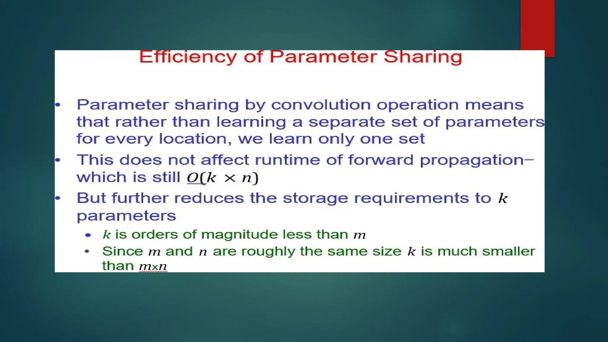
Parameter sharing is used in the convolutional layers to reduce the number of
parameters in the network. For example in the first convolutional layer let’s say we
have an output of 15x15x4 where 15 is the size of the output and 4 the number of
filters used in this layer. For each output node in that layer we have the same filter,
thus reducing dramatically the storage requirements of the model to the size of the
filter.

33. Equivariant Representations

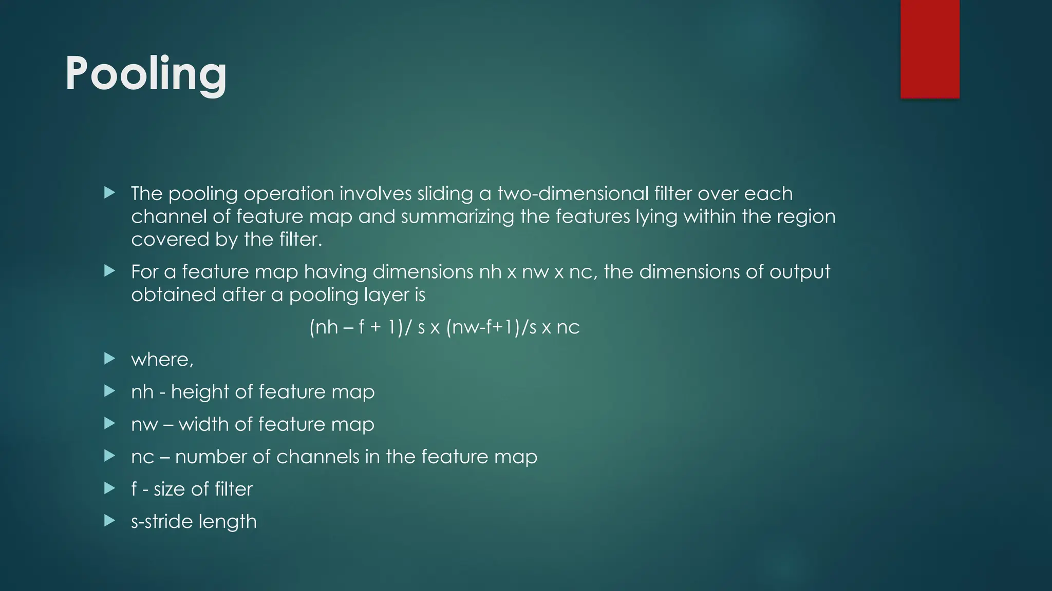
35. Pooling
 The pooling operation involves sliding a two-dimensional filter over each
channel of feature map and summarizing the features lying within the region
covered by the filter.
 For a feature map having dimensions nh x nw x nc, the dimensions of output
obtained after a pooling layer is
(nh – f + 1)/ s x (nw-f+1)/s x nc
 where,
 nh - height of feature map
 nw – width of feature map
 nc – number of channels in the feature map
 f - size of filter
 s-stride length

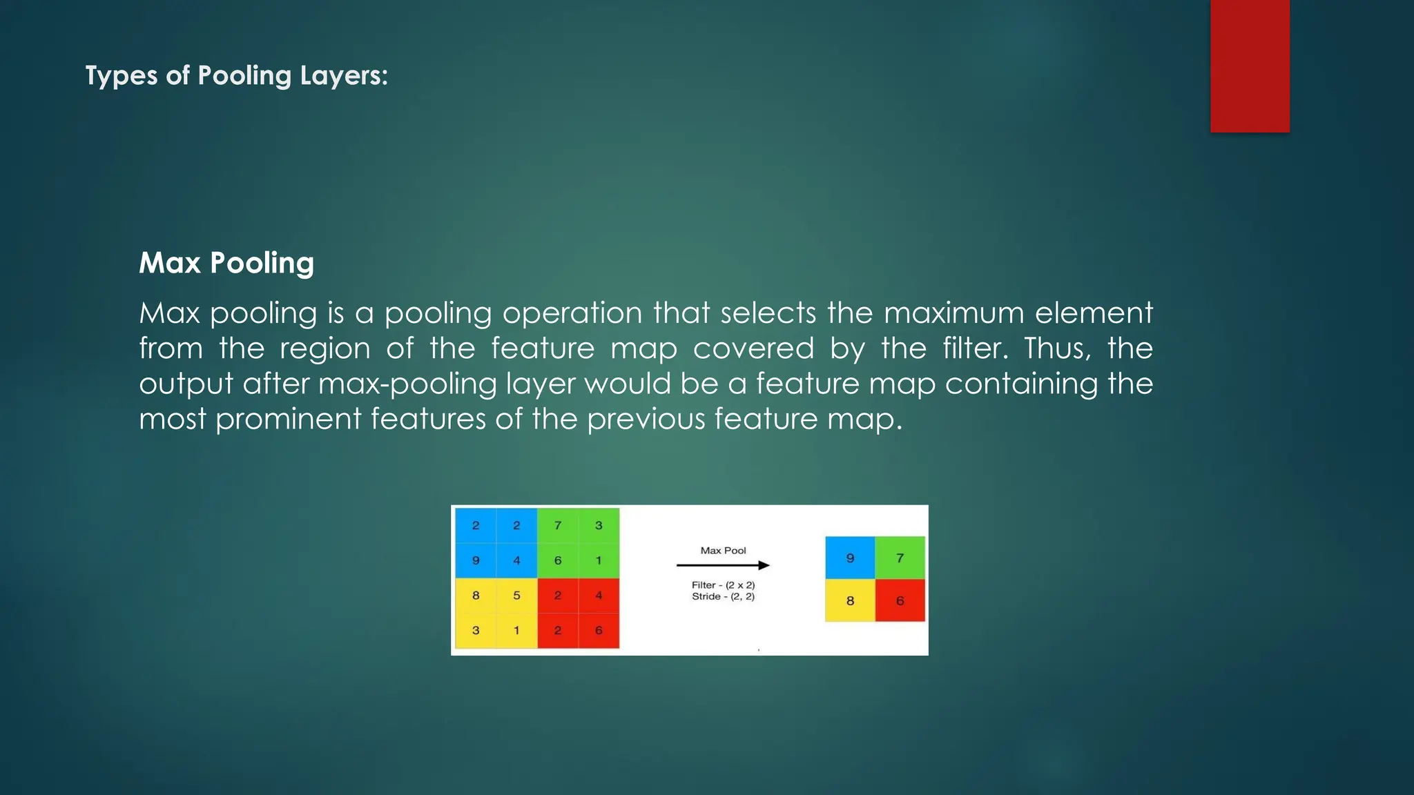
36. Types of Pooling Layers:
Max Pooling
Max pooling is a pooling operation that selects the maximum element
from the region of the feature map covered by the filter. Thus, the
output after max-pooling layer would be a feature map containing the
most prominent features of the previous feature map.

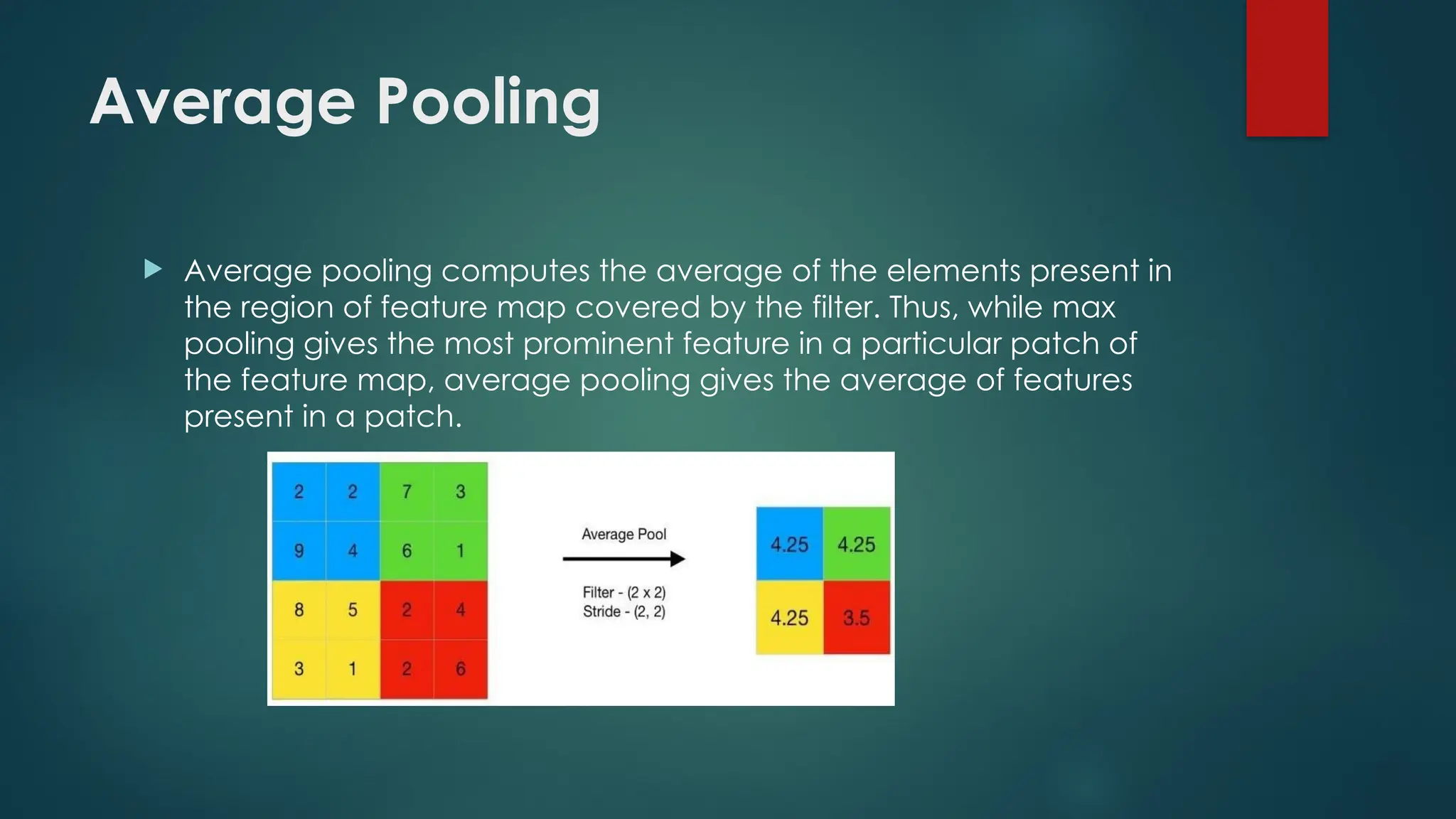
37. Average Pooling
 Average pooling computes the average of the elements present in
the region of feature map covered by the filter. Thus, while max
pooling gives the most prominent feature in a particular patch of
the feature map, average pooling gives the average of features
present in a patch.

38. Global Average Pooling
 Considering a tensor of shape h*w*n, the output of the Global
Average Pooling layer is a single value across h*w that summarizes
the presence of the feature. Instead of downsizing the patches of
the input feature map, the Global Average Pooling layer downsizes
the whole h*w into 1 value by taking the average.

39. Global Max Pooling
 With the tensor of shape h*w*n, the output of the Global Max
Pooling layer is a single value across h*w that summarizes the
presence of a feature. Instead of downsizing the patches of the
input feature map, the Global Max Pooling layer downsizes the
whole h*w into 1 value by taking the maximum.

40.  Convolutional Neural Network (CNN) is an advanced version of
artificial neural networks (ANNs), primarily designed to extract
features from grid-like matrix datasets. This is particularly useful for
visual datasets such as images or videos, where data patterns play
a crucial role. CNNs are widely used in computer vision applications
due to their effectiveness in processing visual data.
 CNNs consist of multiple layers like the input layer, Convolutional
layer, pooling layer, and fully connected layers.

42.  Input Layers: It’s the layer in which we give input to our model. In
CNN, Generally, the input will be an image or a sequence of
images. This layer holds the raw input of the image with width 32,
height 32, and depth 3.
 Convolutional Layers: This is the layer, which is used to extract the
feature from the input dataset. It applies a set of learnable filters
known as the kernels to the input images. The filters/kernels are
smaller matrices usually 2x2, 3x3, or 5x5 shape. it slides over the input
image data and computes the dot product between kernel weight
and the corresponding input image patch. The output of this layer is
referred as feature maps. Suppose we use a total of 12 filters for this
layer we’ll get an output volume of dimension 32 x 32 x 12.

43.  Activation Layer: By adding an activation function to the output of
the preceding layer, activation layers add nonlinearity to the
network. it will apply an element-wise activation function to the
output of the convolution layer. Some common activation functions
are RELU: max(0, x), Tanh, Leaky RELU, etc. The volume remains
unchanged hence output volume will have dimensions 32 x 32 x 12.
 Pooling layer: This layer is periodically inserted in the covnets and its
main function is to reduce the size of volume which makes the
computation fast reduces memory and also prevents overfitting.
Two common types of pooling layers are max pooling and average
pooling. If we use a max pool with 2 x 2 filters and stride 2, the
resultant volume will be of dimension 16x16x12.

44.  Flattening: The resulting feature maps are flattened into a one-
dimensional vector after the convolution and pooling layers so they
can be passed into a completely linked layer for categorization or
regression.
 Fully Connected Layers: It takes the input from the previous layer
and computes the final classification or regression task.

46.  Advantages of CNNs
 Good at detecting patterns and features in images, videos, and
audio signals.
 Robust to translation, rotation, and scaling invariance.
 End-to-end training, no need for manual feature extraction.
 Can handle large amounts of data and achieve high accuracy.

47.  Disadvantages of CNNs
 Computationally expensive to train and require a lot of memory.
 Can be prone to overfitting if not enough data or proper
regularization is used.
 Requires large amounts of labeled data.
 Interpretability is limited, it's hard to understand what the network
has learned.

48. stride
Suppose we choose a stride of 2. So, while convoluting through the
image, we will take two steps – both in the horizontal and vertical
directions separately. The dimensions for stride s will be:
 Input: n X n
 Padding: p
 Stride: s
 Filter size: f X f
 Output: [(n+2p-f)/s+1] X [(n+2p-f)/s+1]
 Stride helps to reduce the size of the image, a particularly useful
feature.

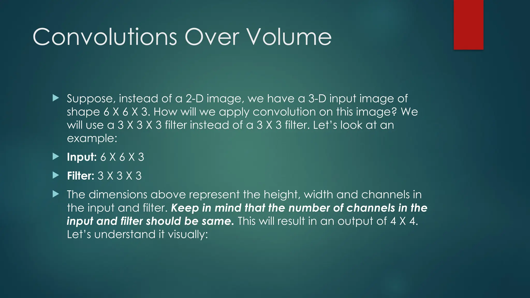
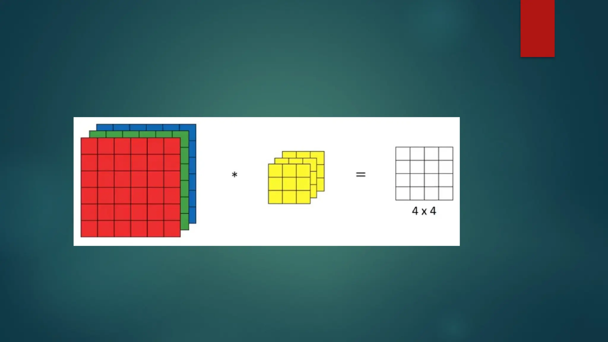
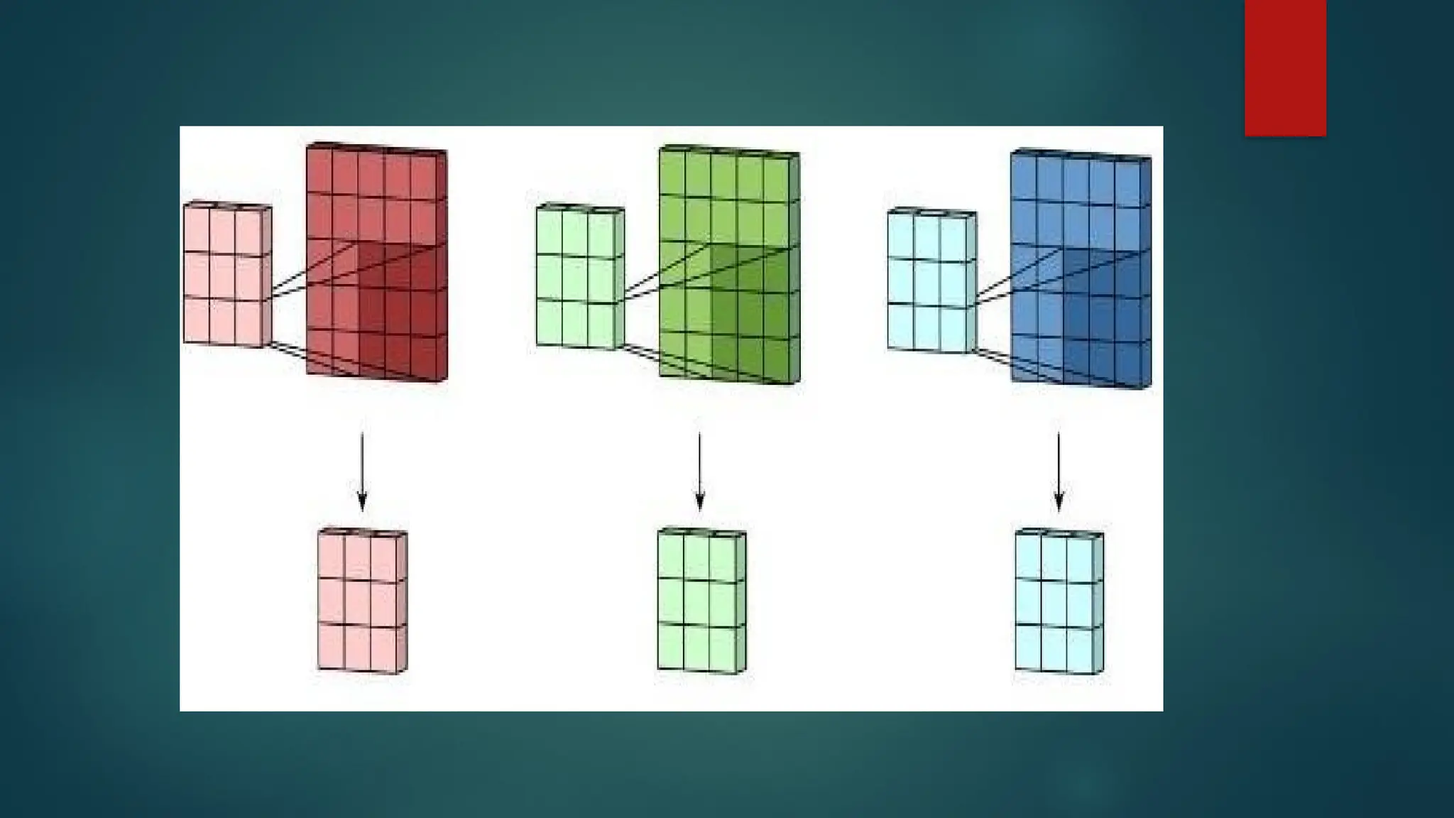
49. Convolutions Over Volume
 Suppose, instead of a 2-D image, we have a 3-D input image of
shape 6 X 6 X 3. How will we apply convolution on this image? We
will use a 3 X 3 X 3 filter instead of a 3 X 3 filter. Let’s look at an
example:
 Input: 6 X 6 X 3
 Filter: 3 X 3 X 3
 The dimensions above represent the height, width and channels in
the input and filter. Keep in mind that the number of channels in the
input and filter should be same. This will result in an output of 4 X 4.
Let’s understand it visually:

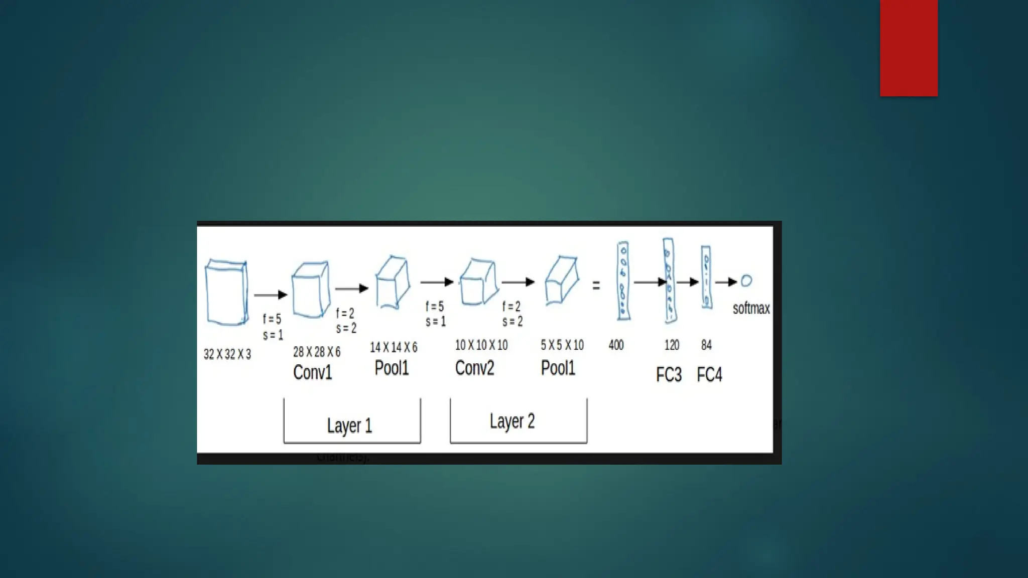
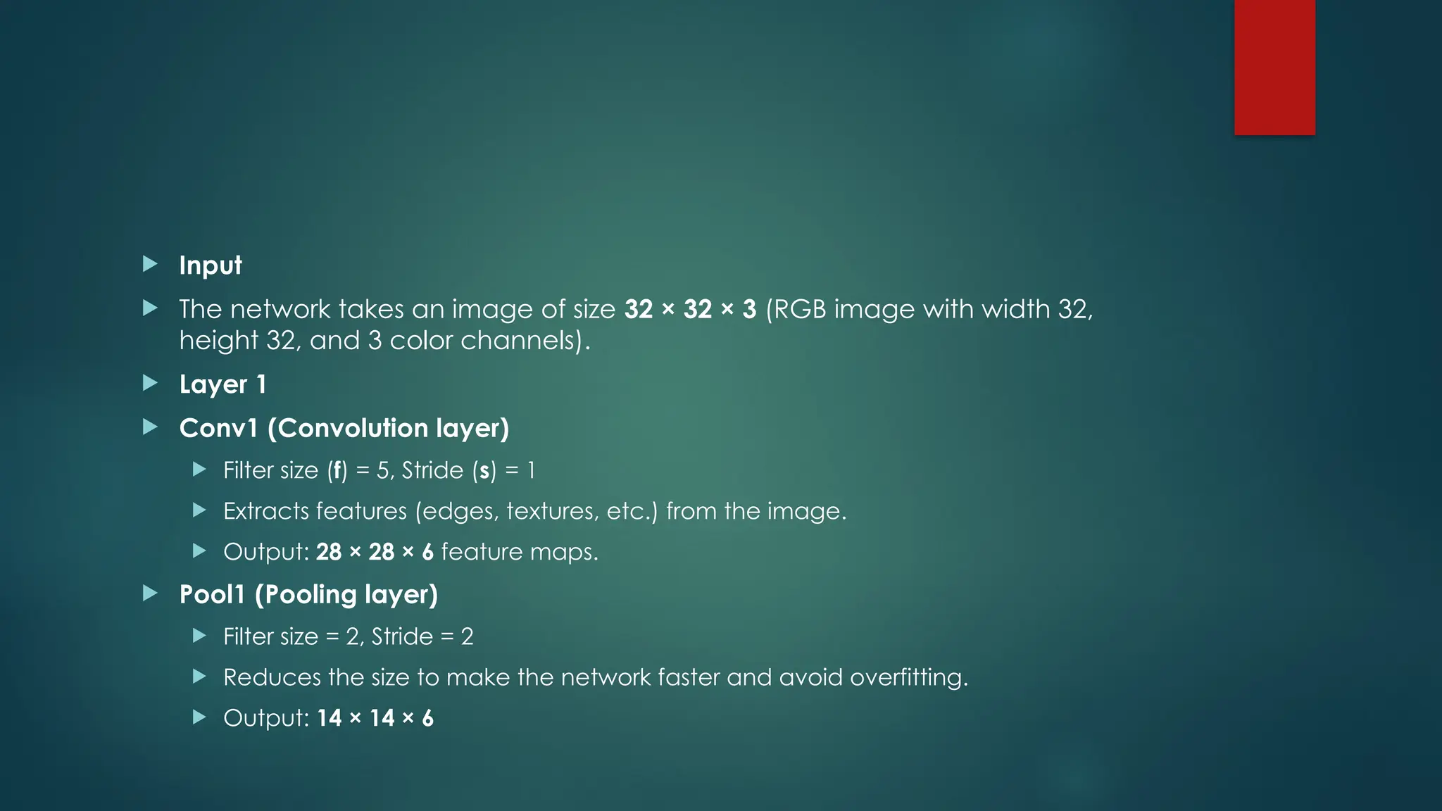
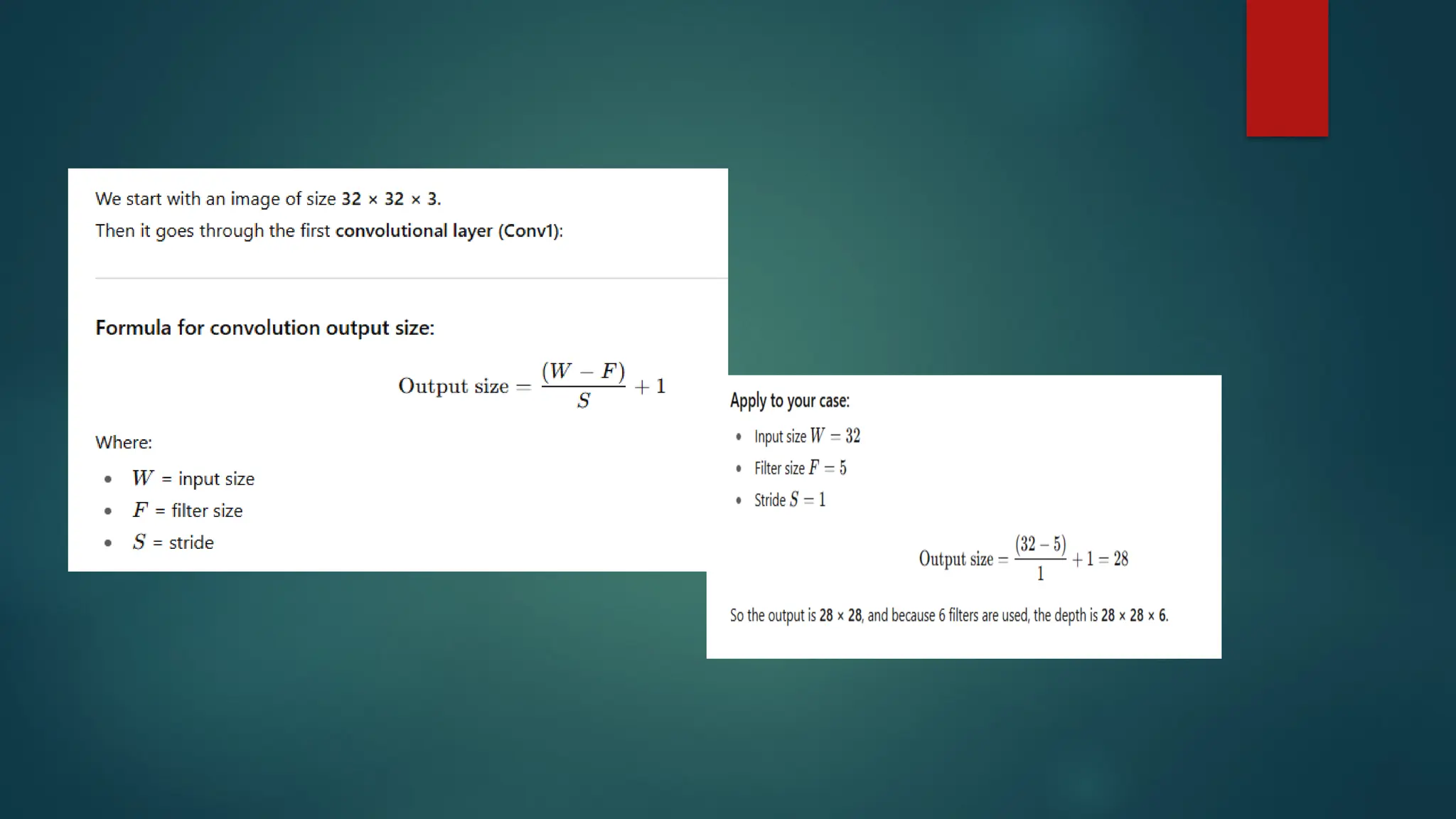
52.  Input
 The network takes an image of size 32 × 32 × 3 (RGB image with width 32,
height 32, and 3 color channels).
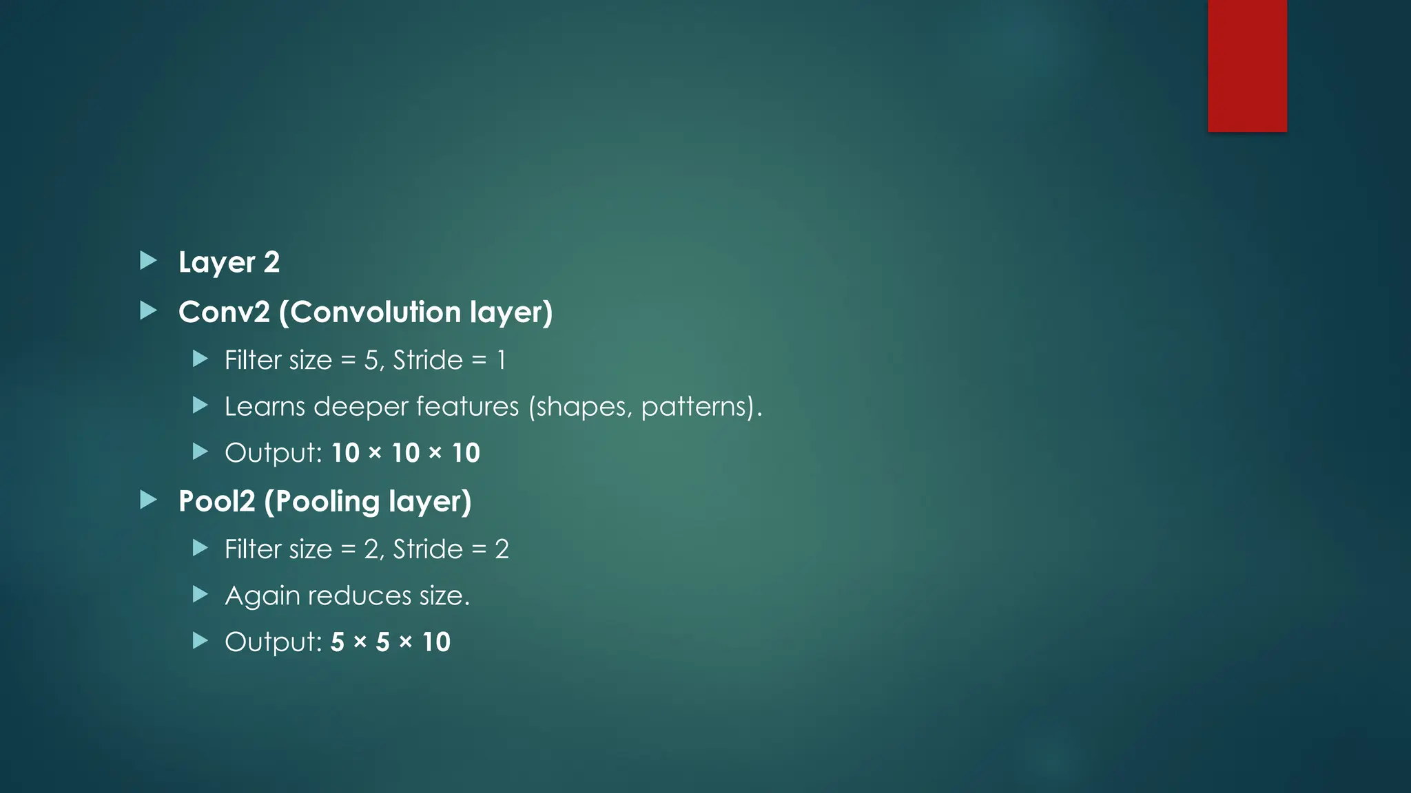
 Layer 1
 Conv1 (Convolution layer)
 Filter size (f) = 5, Stride (s) = 1
 Extracts features (edges, textures, etc.) from the image.
 Output: 28 × 28 × 6 feature maps.
 Pool1 (Pooling layer)
 Filter size = 2, Stride = 2
 Reduces the size to make the network faster and avoid overfitting.
 Output: 14 × 14 × 6

53.  Layer 2
 Conv2 (Convolution layer)
 Filter size = 5, Stride = 1
 Learns deeper features (shapes, patterns).
 Output: 10 × 10 × 10
 Pool2 (Pooling layer)
 Filter size = 2, Stride = 2
 Again reduces size.
 Output: 5 × 5 × 10

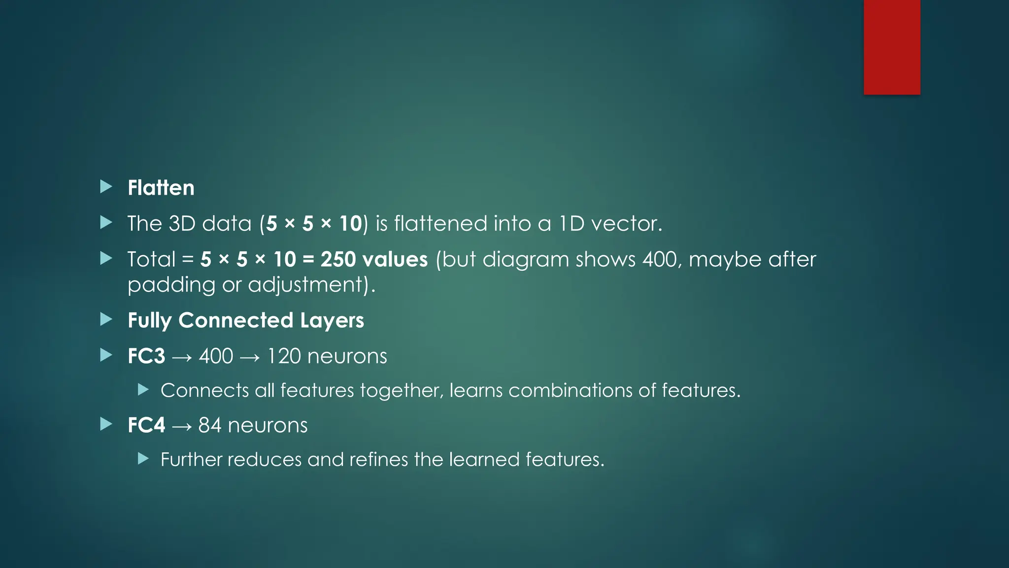
54.  Flatten
 The 3D data (5 × 5 × 10) is flattened into a 1D vector.
 Total = 5 × 5 × 10 = 250 values (but diagram shows 400, maybe after
padding or adjustment).
 Fully Connected Layers
 FC3 → 400 → 120 neurons
 Connects all features together, learns combinations of features.
 FC4 → 84 neurons
 Further reduces and refines the learned features.

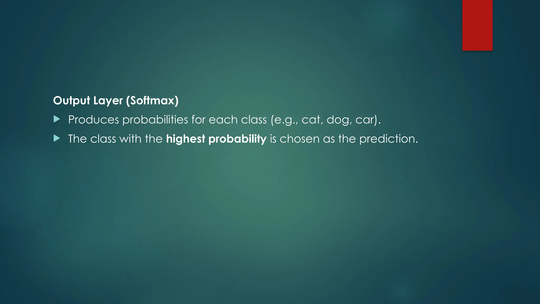
55. Output Layer (Softmax)
 Produces probabilities for each class (e.g., cat, dog, car).
 The class with the highest probability is chosen as the prediction.