Download as PDF, PPTX
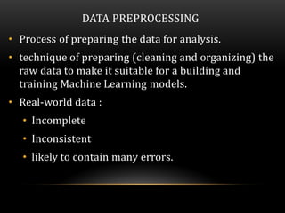
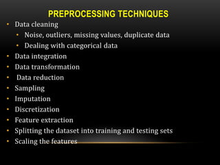
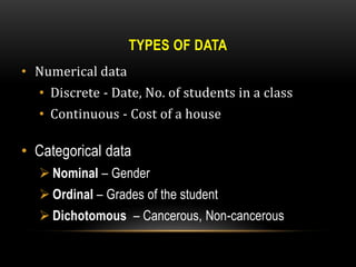
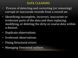
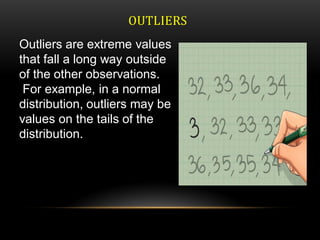

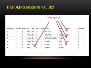
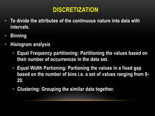
This document discusses various techniques for data preprocessing, which is the process of preparing raw data for analysis by cleaning, transforming, and reducing data. It describes methods for cleaning data by handling missing values, outliers, and duplicates. Techniques covered for transforming data include normalization, discretization, and handling categorical variables. The document also discusses sampling, feature selection, and other methods for reducing dimensions and selecting relevant features from datasets.


![[Deck] What's New in Spark-Iceberg Integration via DSV2.pptx](https://cdn.slidesharecdn.com/ss_thumbnails/deckwhatsnewinspark-icebergintegrationviadsv2-260210005337-25955b12-thumbnail.jpg?width=640&height=640&fit=bounds)


