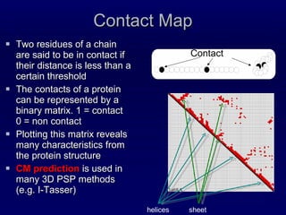
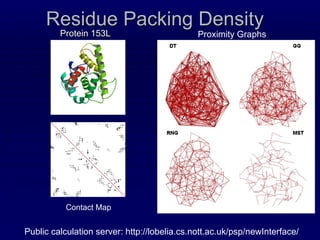
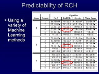
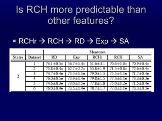
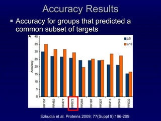
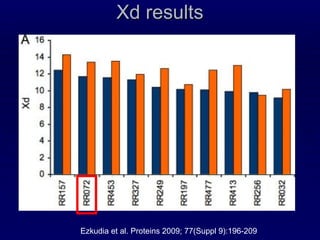
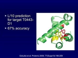
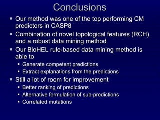
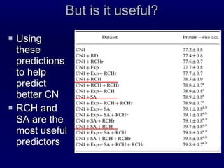
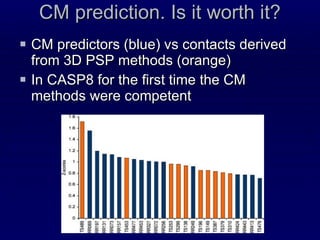
1. The document discusses a contact map prediction method that was one of the top performers in CASP8. It uses topological properties of proteins like recursive convex hulls along with machine learning to predict contacts. 2. The method was tested on CASP8 targets, achieving high accuracy scores. Analysis of the predictive rules provided insights into which features were most important. 3. While performance was good, there is still room for improvement, such as better ranking of predictions or using correlated mutations. The contact map prediction approach is valuable as in CASP8 it was competitive with methods using 3D structure prediction.

1. Data Mining Protein Structures' Topological Properties to Enhance Contact Map Predictions Dr. Jaume Bacardit School of Computer Science and School of Biosciences University of Nottingham [email_address] Weizmann Institute of Sciences, May 27 th , 2010

2. Preface General context of the talk is Protein Structure Prediction (PSP) Specifically, this talk describes our Contact Map (CM) prediction method that was one of the top predictors in the last edition of CASP CASP = Critical Assessment of Techniques for Protein Structure Prediction. Biannual community-wide experiment to assess the state-of-the-art in PSP The use of topological models of protein structure has contributed to better CM prediction

3. Roadmap Protein Structure Prediction (PSP) Topological properties of protein residues (TP) Our contact map predictor (CM) Contact Map Prediction at CASP9 (CASP) What insight can we extract from the method? (INS) PSP  TP  CM  CASP  INS

4. PROTEIN STRUCTURE AND CONTACT MAP PREDICTION PSP  TP  CM  CASP  INS

5. Protein Structure Prediction Protein Structure Prediction (PSP) aims to predict the 3D structure of a protein based on its primary sequence Primary Sequence 3D Structure

6. Why PSP? PSP remains, after many years, one of the main challenges in computational biology The function of a protein is determined by its structure Thus, algorithms for predicting a protein’s structure will aid Understanding a protein’s function and characterising its binding sites Producing antibodies for immunolocalisation And looking far beyond…. designing new proteins (better crops, more efficient drugs, etc.)

7. PSP: A family of problems There are several kinds of prediction problems within the scope of PSP The main one is to predict the 3D coordinates of all atoms of a protein (or at least the backbone) based on its primary sequence There are many structural properties of individual residues within a protein that can be predicted Secondary structure (SS), solvent accessibility (SA) Accurate predictions of these sub-problems are a stepping stone towards the general 3D problem

8. PSP sub-problems Secondary structure prediction The most usual way is to predict whether a residue belongs to an α helix a β sheet or is in coil state Solvent accessibility Predicting the relative surface of each amino acid which is exposed to the solvent Predicted as an absolute measure or partitioned in states (low/high)

9. TOPOLOGICAL PROPERTIES OF PROTEINS PSP  TP  CM  CASP  INS

10. Contact Map Two residues of a chain are said to be in contact if their distance is less than a certain threshold The contacts of a protein can be represented by a binary matrix. 1 = contact 0 = non contact Plotting this matrix reveals many characteristics from the protein structure CM prediction is used in many 3D PSP methods (e.g. I-Tasser) Contact helices sheets

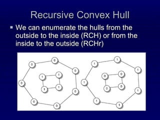
11. Recursive Convex Hull Structural feature that we have proposed recently [Stout, Bacardit, Hirst & Krasnogor, Bioinformatics 2008 24(7):916-923; ] We model a protein as a series of nested layers, assigning each residue to a different layer Strictly speaking each layer is a convex hull of points The convex hull of a point set is simple and fast to compute Recursive Convex Hull is computed by iteratively identifying the layers (hulls) of a protein

12. Recursive Convex Hull We can enumerate the hulls from the outside to the inside (RCH) or from the inside to the outside (RCHr)

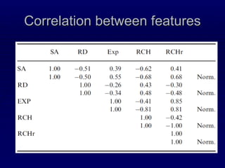
13. Relation of RCH to other structural properties Comparing Solvent Accessiblity Exposure [Ben-Shimon and Eisenstein;05] Residue depth [Chakravarti and Varadarajan;99] RCH/RCHr

14. Correlation between features

15. Proximity Graphs (PGs) DT ⊇ GG ⊇ RNG ⊇ MST Poupon: 2004 Delanuy Tessellation of a point set QHull: Barber, C.B., Dobkin, D.P., and Huhdanpaa, H.T., "The Quickhull algorithm for convex hulls," ACM Trans. on Mathematical Software , 22(4):469-483, Dec 1996

16. Proximity Graphs (PGs) DT ⊇ GG ⊇ RNG ⊇ MST Minimum Spanning Tree (MST) Search for shortest path in RNG Remove edges from DT if a sphere drawn between the vertices contains another vertex  Gabriel Graph (GG) Remove edges from GG if an sherical lune contains another vertex  Relative Neighbourhood Graph (RNG)

17. Residue Packing Density Protein 153L Proximity Graphs Contact Map Public calculation server: http://lobelia.cs.nott.ac.uk/psp/newInterface/

18. Predictability of RCH We predicted the RCH of a residue using a window of ±4 amino acids around it including: AA types of the residues Predicted secondary structure Average predicted RCH for the whole chain The distribution of RCH values was partitioned into 2, 3 and 5 states

19. Predictability of RCH Using a variety of Machine Learning methods

20. Is RCH more predictable than other features? RCHr  RCH  RD  Exp  SA

21. But is it useful? Using these predictions to help predict better CN RCH and SA are the most useful predictors

22. OUR CONTACT MAP PREDICTION METHOD PSP  TP  CM  CASP  INS

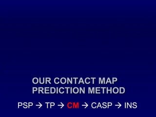
23. Steps Prediction of Secondary structure (using PSIPRED) Solvent Accessibility Recursive Convex Hull Coordination Number Integration of all these predictions plus other sources of information Final CM prediction (using BioHEL) Using BioHEL [Bacardit et al., 09]

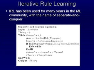
24. The BioHEL GBML System BIOinformatics-oriented Hiearchical Evolutionary Learning – BioHEL (Bacardit et al., 2007) BioHEL is a rule-based evolutionary learning system that employs the Iterative Rule Learning (IRL) paradigm First used in EC in Venturini’s SIA system (Venturini, 1993) Widely used for both Fuzzy and non-fuzzy evolutionary learning BioHEL inherits most of its components from GAssist [Bacardit, 04], a Pittsburgh evolutionary learning system

25. Iterative Rule Learning IRL has been used for many years in the ML community, with the name of separate-and-conquer

26. Characteristics of BioHEL A fitness function based on the Minimum-Description-Length (MDL) (Rissanen,1978) principle that tries to Evolve accurate rules Evolve high coverage rules Evolve rules with low complexity, as general as possible The Attribute List Knowledge representation Representation designed to efficiently handle high-dimensionality domains The ILAS windowing scheme Efficiency enhancement method, not all training points are used for each fitness computation An explicit default rule mechanism Generating more compact rule sets Ensembles for consensus prediction Easy system to boost robustness

27. Prediction of RCH, SA and CN We selected a set of 2811 protein chains from PDB-REPRDB with: A resolution less than 2Å Less than 30% sequence identify Without chain breaks nor non-standard residues 90% of this set was used for training (~490000 residues) 10% for test

28. How are these features predicted? Many of these features are due to local interactions of an amino acid and its immediate neighbours We predict them from the closest neighbours in the chain R i SS i R i+1 SS i+1 R i-1 SS i-1 R i+2 SS i+2 R i-2 SS i-2 R i+3 SS i+3 R i+4 SS i+4 R i-3 SS i-3 R i-4 SS i-4 R i-5 SS i-5 R i+5 SS i+5 R i-1 R i R i+1  SS i R i R i+1 R i+2  SS i+1 R i+1 R i+2 R i+3  SS i+2

29. Prediction of RCH, SA and CN All three features were predicted based on a window of ±4 residues around the target Evolutionary information (as a Position-Specific Scoring Matrix) is the basis of this local information Each residue characterised by a vector of 180 values The domain for all three features was partitioned into 5 states

30. Characterisation of the contact map problem Three types of input information were used Detailed information of three different windows of residues centered around The two target residues (2x) The middle point between them Information about the connecting segment between the two target residues and Global protein information. 1 2 3

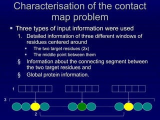
31. 1. Three windows of residues Two windows of ±4 residues around the two target amino-acids One window of ±2 residues around the middle point in the chain between the two targets [Punta and Rost, 05] Each position in all three windows contains: PSSM profile (from PSI-BLAST) Predicted SS, SA, RCH and CN

32. Description of connecting segment and the whole sequence 2. The segments are described by the distribution of Amino acid types Predicted SS, RCH, SA and CN [Punta and Rost, 05] 3. Other information Sequence length Separation between targets Contact propensity between the amino acid types of the targets [Shackelford and Karplus, 07]

33. Contact Map dataset The set of 2811 proteins was randomly halved Moreover, all proteins with more than 350 amino acids were discarded Still, the resulting training set contained more than 15.2 million instances and 631 attributes Less than 2% of those are actual contacts 36GB of disk space

34. Samples and ensembles 50 samples of 300K examples are generated from the training set with a ratio of 2:1 non-contacts/contacts BioHEL is run 25 times for each sample Prediction is done by a consensus of 1250 rule sets Confidence of prediction is computed based on the votes distribution in the ensemble. Whole training process takes about 289 CPU days (~5.5h/rule set) Training set x50 x25 Consensus Predictions Samples Rule sets

35. CONTACT MAP PREDICTION AT CASP9 PSP  TP  CM  CASP  INS

36. Contact Map prediction in CASP Contact Map is assessed using the 11 CASP targets in the Free Modelling category Also, only long-range contacts (with a minimum chain separation of 24 residues) are evaluated Predictor groups are asked to submit a list of predicted contacts and a confidence level for each prediction The assessors then rank the predictions for each protein and take a look at the top L/x ones, where L is the length of the protein and x={5,10}

37. Contact Map prediction in CASP From these L/x top ranked contacts two measures are computed Accuracy: TP/(TP+FP) Xd: difference between the distribution of predicted distance and a random distribution 22 groups participated in casp8, but not all of them sent enough predictions for L/10 or L/5

38. Accuracy Results Accuracy for groups that predicted a common subset of targets Ezkudia et al. Proteins 2009; 77(Suppl 9):196-209

39. Xd results Ezkudia et al. Proteins 2009; 77(Suppl 9):196-209

40. L/10 prediction for target T0443-D1 67% accuracy Ezkudia et al. Proteins 2009; 77(Suppl 9):196-209

41. WHAT INSIGHT CAN WE EXTRACT FROM THE METHOD? PSP  TP  CM  CASP  INS

42. Is all that information useful? Many different types of information were used to perform the prediction Is all of it relevant? As BioHEL generates human-readable sets of rules we can address this question

43. Rule generated by BioHEL Att PredSS_r1_1 is E,X and Att PredRCH_r1 is 4 Att PredCN_r1_-1 is 0,2,3,4,X and Att PredCN_r2_1 is 3,4 and Att AA_freq_central_P=0 and Att AA_freq_global_E is [0.02,0.10] and Att PSSM_r2_-1_Y is [-7,9.69] and Att PSSM_r2_0_I is [1.76,8] then contact 8 attributes in this rule out of 631 (in average 8.3 att/rule)

44. Understanding the rule sets Each rule set has in average 135 rules We have a total of 168470 rules Impossible to read all of them individually, but we can extract useful statistics For instance, how often was each attribute used in the rules?

45. Distribution of frequency of use of attributes All 631 attributes are actually used (min frequency=429) However, some of them are used much more frequently than others

46. Top 10 attributes The four kind of residue’s predictions are highly ranked Attribute Frequency Counts PredSS_r1_1 1.48% 18141 PredCN_r1 1.66% 20336 propensity 1.74% 21288 PredSS_r2 1.75% 21350 PredSS_r1 1.82% 22205 PredRCH_r2 1.87% 22856 PredRCH_r1 2.04% 24961 PredSA_r2 2.12% 25891 PredSA_r1 2.39% 29246 separation 4.17% 50951

47. Beyond individual attributes… We can also identify when certain pairs (or triplets) of attributes appear always together in rules Rules for alpha helices or beta sheets And not just take a look at the attributes, but also at the actual patterns of predicates

48. Conclusions Our method was one of the top performing CM predictors in CASP8 Combination of novel topological features (RCH) and a robust data mining method Our BioHEL rule-based data mining method is able to Generate competent predictions Extract explanations from the predictions Still a lot of room for improvement Better ranking of predictions Alternative formulation of sub-predictions Correlated mutations

49. CM prediction. Is it worth it? CM predictors (blue) vs contacts derived from 3D PSP methods (orange) In CASP8 for the first time the CM methods were competent

50. Acknowledgements Many thanks to the members of our Infobiotics team in CASP8 Prof. Natalio Krasnogor Prof. Jonathan Hirst Dr. Michael Stout The UK Engineering and Physical Sciences Research Council (EPSRC) under grant GR/T07534/01 The University of Nottingham’s High Performance Computing cluster