Courses_Advanced Statistics (14-15).pptx

RMCIII Quantitative Analysis
Basic and Advanced Statistics
Dr Matthew Carter

Session Outline
Lecture – Meeting Room (Morning)
Basic Statistics
Part 1: Research Design
Part 2: Descriptive Statistics
Lecture – Meeting Room (Afternoon)
Advanced Statistics
Part 1: Inferential Statistics
Part 2: Choosing a Statistical Test
Workshop – Computer Lab (Monday)
Worked examples using SPSS

Part 1: Inferential Statistics

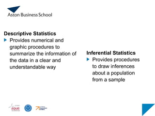
Descriptive Statistics
Provides numerical and
graphic procedures to
summarize the information of
the data in a clear and
understandable way
Inferential Statistics
Provides procedures
to draw inferences
about a population
from a sample

Inferential Statistics
Inferential statistics are used to draw conclusions about a
population by examining a sample.
POPULATION
Sample

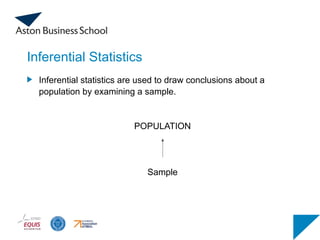
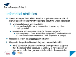
Inferential statistics
Select a sample from within the total population with the aim of
drawing an inference from this sample about the wider population
what population are we interested in
e.g. nursing staff turnover – population is nurses not other
healthcare staff
draw sample that is representative (or risk sampling error)
e.g. comparing doctors and nurses – population 2000 nurses and
500 doctors (4-to-1) then ensure same proportion in sample
Necessary to set up hypothesis in advance
Calculate the probability obtaining such as a relationship
If the calculated probability is small enough then it suggests
that the relationship observed is unlikely to have arisen by
chance so reflects a genuine relationship in the population

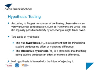
Hypothesis Testing
According to Popper no number of confirming observations can
verify universal generalization, such as ‘All swans are white’, yet
it is logically possible to falsify by observing a single black swan.
Two types of hypothesis
The null hypothesis, H0, is a statement that the thing being
studied produces no effect or makes no difference.
The alternative hypothesis, Ha, is a statement that the thing
being studied produces an effect or makes a difference.
Null hypothesis is framed with the intent of rejecting it.

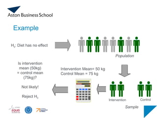
Example
H0: “This diet has no effect on people's weight."
Ha : “This diet has an effect on people's weight."

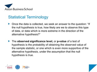
Statistical Terminology
Once the data is collected, we seek an answer to the question: “If
the null hypothesis is true, how likely are we to observe this type
of data, or data which is more extreme in the direction of the
alternative hypothesis?”
The observed significance level, or p-value of a test of
hypothesis is the probability of obtaining the observed value of
the sample statistic, or one which is even more supportive of the
alternative hypothesis, under the assumption that the null
hypothesis is true.

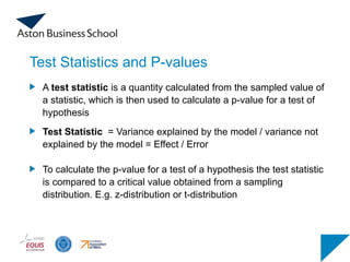
Test Statistics and P-values
A test statistic is a quantity calculated from the sampled value of
a statistic, which is then used to calculate a p-value for a test of
hypothesis
Test Statistic = Variance explained by the model / variance not
explained by the model = Effect / Error
To calculate the p-value for a test of a hypothesis the test statistic
is compared to a critical value obtained from a sampling
distribution. E.g. z-distribution or t-distribution

Example
Population
H0: Diet has no effect
Intervention Mean= 50 kg
Control Mean = 75 kg
Sample
Is intervention
mean (50kg)
= control mean
(75kg)?
Not likely!
Reject H0
Control
Intervention

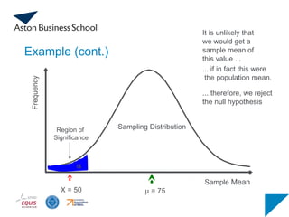
Example (cont.)
Sample Mean
m = 75
Sampling Distribution
It is unlikely that
we would get a
sample mean of
this value ...
... if in fact this were
the population mean.
... therefore, we reject
the null hypothesis
X = 50
Frequency
a
Region of
Significance

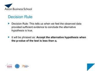
Decision Rule
Decision Rule: This tells us when we feel the observed data
provided sufficient evidence to conclude the alternative
hypothesis is true.
It will be phrased as: Accept the alternative hypothesis when
the p-value of the test is less than a.

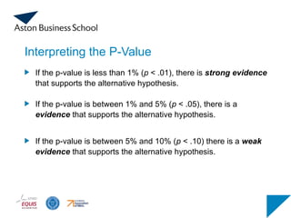
Interpreting the P-Value
If the p-value is less than 1% (p < .01), there is strong evidence
that supports the alternative hypothesis.
If the p-value is between 1% and 5% (p < .05), there is a
evidence that supports the alternative hypothesis.
If the p-value is between 5% and 10% (p < .10) there is a weak
evidence that supports the alternative hypothesis.

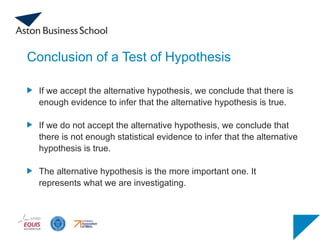
Conclusion of a Test of Hypothesis
If we accept the alternative hypothesis, we conclude that there is
enough evidence to infer that the alternative hypothesis is true.
If we do not accept the alternative hypothesis, we conclude that
there is not enough statistical evidence to infer that the alternative
hypothesis is true.
The alternative hypothesis is the more important one. It
represents what we are investigating.

Possible Errors
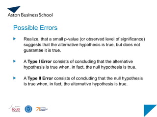
Realize, that a small p-value (or observed level of significance)
suggests that the alternative hypothesis is true, but does not
guarantee it is true.
A Type I Error consists of concluding that the alternative
hypothesis is true when, in fact, the null hypothesis is true.
A Type II Error consists of concluding that the null hypothesis
is true when, in fact, the alternative hypothesis is true.

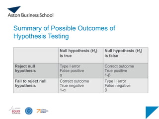
Summary of Possible Outcomes of
Hypothesis Testing
Null hypothesis (H0)
is true
Null hypothesis (H0)
is false
Reject null
hypothesis
Type I error
False positive
α
Correct outcome
True positive
1-β
Fail to reject null
hypothesis
Correct outcome
True negative
1-α
Type II error
False negative
β

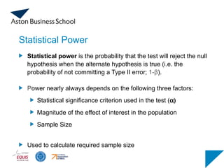
Statistical Power
Statistical power is the probability that the test will reject the null
hypothesis when the alternate hypothesis is true (i.e. the
probability of not committing a Type II error; 1-β).
Power nearly always depends on the following three factors:
Statistical significance criterion used in the test (a)
Magnitude of the effect of interest in the population
Sample Size
Used to calculate required sample size

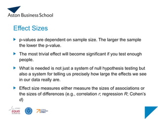
Effect Sizes
p-values are dependent on sample size. The larger the sample
the lower the p-value.
The most trivial effect will become significant if you test enough
people.
What is needed is not just a system of null hypothesis testing but
also a system for telling us precisely how large the effects we see
in our data really are.
Effect size measures either measure the sizes of associations or
the sizes of differences (e.g., correlation r; regression R; Cohen’s
d)

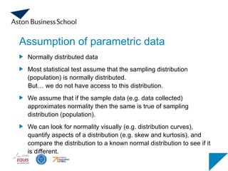
Assumption of parametric data
Normally distributed data
Most statistical test assume that the sampling distribution
(population) is normally distributed.
But… we do not have access to this distribution.
We assume that if the sample data (e.g. data collected)
approximates normality then the same is true of sampling
distribution (population).
We can look for normality visually (e.g. distribution curves),
quantify aspects of a distribution (e.g. skew and kurtosis), and
compare the distribution to a known normal distribution to see if it
is different.

Part 2: Choosing a Statistical Test

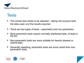
Tests
The correct test needs to be selected – taking into account both
the data used, and the results required.
There are two types of tests – parametric and non-parametric.
Most parametric tests require normally distributed data, at least in
the DV.
Non-parametric tests are more suitable for heavily skewed or
ordinal data.
Generally speaking, parametric tests are more useful than non-
parametric tests.

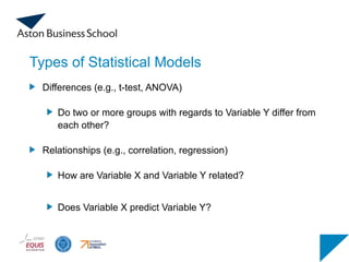
Types of Statistical Models
Differences (e.g., t-test, ANOVA)
Do two or more groups with regards to Variable Y differ from
each other?
Relationships (e.g., correlation, regression)
How are Variable X and Variable Y related?
Does Variable X predict Variable Y?

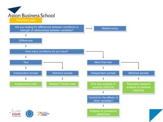
How many conditions do you have?
Are you testing for differences between conditions or
strength of relationships between variables?
Differences
Relationships
Two More than two
Independent sample
Independent t-test
Matched sample
Related / Paired t-test
Parametric data
Independent sample Matched sample
One way analysis of
variance (ANOVA)
Repeated measure
analysis of variance
(ANOVA)
Analysis of covariance
(ANCOVA)
Control for the effects of
other variables?

Key Statistics
Mean
Standard deviation
t-value
p-level

Key Statistics
Means
Standard Deviations
F-statistic
p-level
Post hoc comparison test

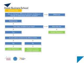
How many variables do you have?
Are you testing for differences between conditions or
strength of relationships between variables?
Relationships
Differences
Two
More than two
Do you want to control for the effects of other
variables?
Linear Regression
Yes
Pearson’s product
moment correlation
Parametric data
No
Multiple Regression

Correlation
Correlation analysis is used to measure strength of the
association (linear relationship) between two variables
Only concerned with strength of the relationship
No causal effect is implied

Scatter Plot Examples
IQ
Exam
grade
110 40
109 39
110 41
114 45
115 46
116 46
117 46
117 48
118 53
119 55
120 55
120 57
119 58
121 60
124 61
125 62
124 64
126 64
126 65
126 68
128 69
132 74
134 75
100 105 110 115 120 125 130 135 140
0
10
20
30
40
50
60
70
80
IQ
Exam
Grade
Linear relationship

Key Statistics
Correlation coefficient r
• |r| = .1 small effect
• |r| = .3 medium effect
• |r| = .5 large effect
p-value

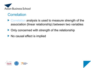
Correlation Coefficient
The sample correlation coefficient (Pearson product-moment
correlation) r is a measure of the strength of the
association between the two variables.
Sample correlation coefficient (algebraic):
(continued)
where:
r = sample correlation coefficient
n = sample size
x = value of the independent variable
y = value of the dependent variable
   
  




]
y)
(
)
y
][n(
x)
(
)
x
[n(
y
x
xy
n
r
2
2
2
2
(rho) is the linear correlation
coefficient for all paired data in
the population.

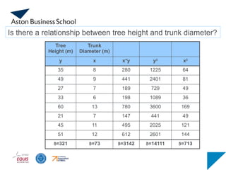
Tree
Height (m)
Trunk
Diameter (m)
y x x*y y2
x2
35 8 280 1225 64
49 9 441 2401 81
27 7 189 729 49
33 6 198 1089 36
60 13 780 3600 169
21 7 147 441 49
45 11 495 2025 121
51 12 612 2601 144
=321 =73 =3142 =14111 =713
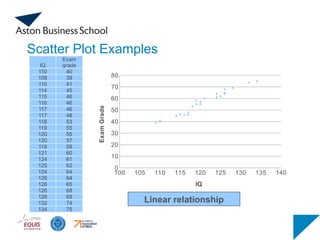
Is there a relationship between tree height and trunk diameter?

0
10
20
30
40
50
60
70
0 2 4 6 8 10 12 14
0.886
]
(321)
][8(14111)
(73)
[8(713)
(73)(321)
8(3142)
]
y)
(
)
y
][n(
x)
(
)
x
[n(
y
x
xy
n
r
2
2
2
2
2
2









   
  
Trunk Diameter, x
Tree
Height,
y
(continued)
r = 0.886 → strong positive
linear association between x and y
variance explained (r2) = - 0.886 *
0.886 = 0.785

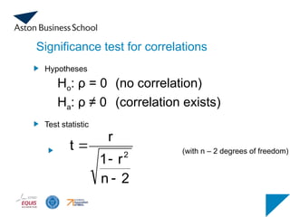
Significance test for correlations
Hypotheses
Ho: ρ = 0 (no correlation)
Ha: ρ ≠ 0 (correlation exists)
Test statistic
(with n – 2 degrees of freedom)
2
n
r
1
r
t
2




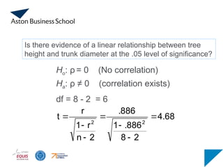
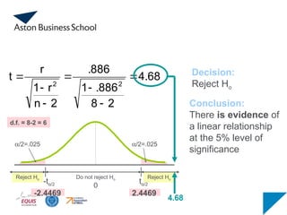
Is there evidence of a linear relationship between tree
height and trunk diameter at the .05 level of significance?
Ho: ρ = 0 (No correlation)
Ha: ρ ≠ 0 (correlation exists)
df = 8 - 2 = 6
4.68
2
8
.886
1
.886
2
n
r
1
r
t
2
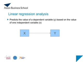
2








4.68
2
8
.886
1
.886
2
n
r
1
r
t
2
2







Conclusion:
There is evidence of
a linear relationship
at the 5% level of
significance
Decision:
Reject Ho
Reject Ho
Reject Ho
a/2=.025
-tα/2
Do not reject Ho
0
tα/2
a/2=.025
-2.4469 2.4469
4.68
d.f. = 8-2 = 6

Linear regression analysis
X Y
Predicts the value of a dependent variable (y) based on the value
of one independent variable (x)

Key Statistics
Unstandardized regression coefficient (b)
Standardized regression coefficient (β)
Standard error (s.e.)
t-statistic
Explained Variance (R2
)

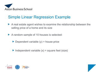
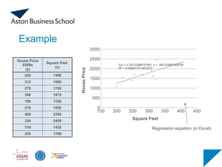
Simple Linear Regression Example
A real estate agent wishes to examine the relationship between the
selling price of a home and its size
A random sample of 10 houses is selected:
Dependent variable (y) = house price
Independent variable (x) = square feet (size)

150 200 250 300 350 400 450
0
500
1000
1500
2000
2500
3000
f(x) = 5.29132988757841 x + 199.033987208785
R² = 0.580817311872272
Square Feet
House
Price
House Price
£000s
(y)
Square Feet
(x)
245 1400
312 1600
279 1700
308 1875
199 1100
219 1550
405 2350
324 2450
319 1425
255 1700
Regression equation (in Excel)
Example

ε
x
β
β
y 1
0 


Linear component
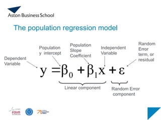
The population regression model
Population
y intercept
Population
Slope
Coefficient
Random
Error
term, or
residual
Dependent
Variable
Independent
Variable
Random Error
component

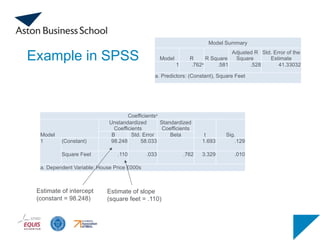
Model Summary
Model R R Square
Adjusted R
Square
Std. Error of the
Estimate
1 .762a
.581 .528 41.33032
a. Predictors: (Constant), Square Feet
Coefficientsa
Model
Unstandardized
Coefficients
Standardized
Coefficients
t Sig.
B Std. Error Beta
1 (Constant) 98.248 58.033 1.693 .129
Square Feet .110 .033 .762 3.329 .010
a. Dependent Variable: House Price £000s
Estimate of intercept
(constant = 98.248)
Estimate of slope
(square feet = .110)
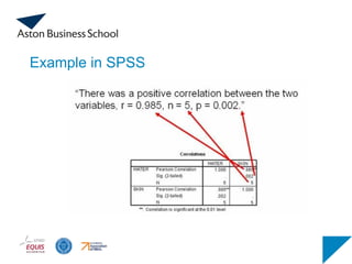
Example in SPSS

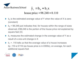
b0 is the estimated average value of Y when the value of X is zero
(constant)
b0 = 98.248 just indicates that, for houses within the range of sizes
observed, £98,248 is the portion of the house price not explained by
square feet (X)
b1 measures the estimated change in the average value of Y as a
result of a one-unit change in X
b1 = .110 tells us that the average value of a house increases
by .110 or £110 (as house price is in £000s), on average, for each
additional square foot
0.110
98.248
price
house 

x
b
b
ŷ 1
0
i 


Model Summary
Model R R Square
Adjusted R
Square
Std. Error of the
Estimate
1 .762a
.581 .528 41.33032
a. Predictors: (Constant), Square Feet
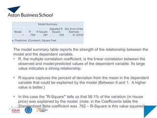
The model summary table reports the strength of the relationship between the
model and the dependent variable.
• R, the multiple correlation coefficient, is the linear correlation between the
observed and model-predicted values of the dependent variable. Its large
value indicates a strong relationship.
• R-square captures the percent of deviation from the mean in the dependent
variable that could be explained by the model (Between 0 and 1. A higher
value is better.)
• In this case the "R-Square"' tells us that 58.1% of the variation (in house
price) was explained by the model. (note: in the Coefficients table the
Standardised Beta coefficient was .762 – R-Square is this value squared)

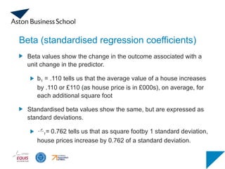
Beta (standardised regression coefficients)
Beta values show the change in the outcome associated with a
unit change in the predictor.
b1 = .110 tells us that the average value of a house increases
by .110 or £110 (as house price is in £000s), on average, for
each additional square foot
Standardised beta values show the same, but are expressed as
standard deviations.
1= 0.762 tells us that as square footby 1 standard deviation,
house prices increase by 0.762 of a standard deviation.

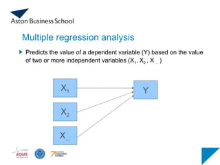
Multiple regression analysis
X1 Y
Predicts the value of a dependent variable (Y) based on the value
of two or more independent variables (X1, X2 , X … )
X2
X…

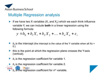
Multiple Regression analysis
If we have two X variables (X1 and X2) which we each think influence
variable Y, we can include both in a linear regression using the
following formula:
b0 is the intercept (the intercept is the value of the Y variable when all Xs =
0.)
this is the point at which the regression plane crosses the Y-axis
(vertical).
b1 is the regression coefficient for variable 1.
b2 is the regression coefficient for variable 2.
bn is the regression coefficient for nth
variable.
i
n
n X
b
X
b
X
b
b
y 





 
2
2
1
1
0

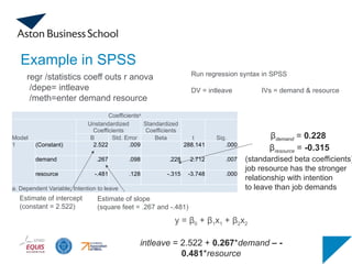
Example in SPSS
regr /statistics coeff outs r anova
/depe= intleave
/meth=enter demand resource
Run regression syntax in SPSS
DV = intleave IVs = demand & resource
Coefficientsa
Model
Unstandardized
Coefficients
Standardized
Coefficients
t Sig.
B Std. Error Beta
1 (Constant) 2.522 .009 288.141 .000
demand .267 .098 .228 2.712 .007
resource -.481 .128 -.315 -3.748 .000
a. Dependent Variable: Intention to leave
Estimate of intercept
(constant = 2.522)
Estimate of slope
(square feet = .267 and -.481)
y = β0 + β1x1 + β2x2
intleave = 2.522 + 0.267*demand – -
0.481*resource
βdemand = 0.228
βresource = -0.315
(standardised beta coefficients)
job resource has the stronger
relationship with intention
to leave than job demands

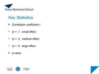
Mediation
A mediator is “[a variable] which represents the generative
mechanism through which the focal [independent] variable is able
to influence the dependent variable of interest” (Baron and
Kenny, 1986).
Independent
Variable (IV)
Mediator Dependent
Variable (DV)

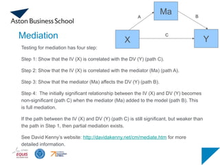
Mediation
Testing for mediation has four step:
Step 1: Show that the IV (X) is correlated with the DV (Y) (path C).
Step 2: Show that the IV (X) is correlated with the mediator (Ma) (path A).
Step 3: Show that the mediator (Ma) affects the DV (Y) (path B).
Step 4: The initially significant relationship between the IV (X) and DV (Y) becomes
non-significant (path C) when the mediator (Ma) added to the model (path B). This
is full mediation.
If the path between the IV (X) and DV (Y) (path C) is still significant, but weaker than
the path in Step 1, then partial mediation exists.
See David Kenny’s website: http://davidakenny.net/cm/mediate.htm for more
detailed information.
Ma
Y
X
A B
C

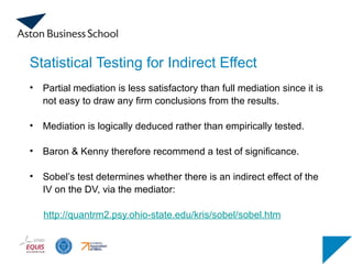
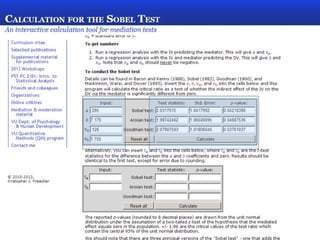
Statistical Testing for Indirect Effect
• Partial mediation is less satisfactory than full mediation since it is
not easy to draw any firm conclusions from the results.
• Mediation is logically deduced rather than empirically tested.
• Baron & Kenny therefore recommend a test of significance.
• Sobel’s test determines whether there is an indirect effect of the
IV on the DV, via the mediator:
http://quantrm2.psy.ohio-state.edu/kris/sobel/sobel.htm

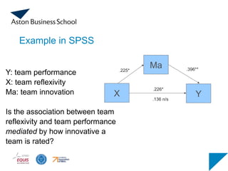
Example in SPSS
X Y
Ma
Y: team performance
X: team reflexivity
Ma: team innovation
Is the association between team
reflexivity and team performance
mediated by how innovative a
team is rated?
.226*
.225* .396**
.136 n/s

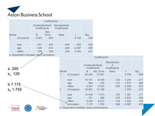
Coefficientsa
Model
Unstandardized
Coefficients
Standardized
Coefficients
t Sig.
B
Std.
Error Beta
1 (Constant) 4.003 .650 6.163 .000
size -.041 .440 -.009 -.093 .926
age -.040 .015 -.269 -2.687 .008
reflex .295 .126 .225 2.340 .021
a. Dependent Variable: team innovation
Coefficientsa
Model
Unstandardized
Coefficients
Standardize
d
Coefficients
t Sig.
B Std. Error Beta
1 (Constant) 45.284 12.051 3.758 .000
size 10.161 8.169 .126 1.244 .217
age .464 .276 .172 1.679 .096
reflex 5.347 2.337 .226 2.289 .024
2 (Constant) 16.561 13.198 1.255 .213
size 10.455 7.573 .130 1.381 .171
age .751 .266 .278 2.827 .006
reflex 3.233 2.227 .136 1.452 .150
innovation 7.175 1.755 .396 4.087 .000
a. Dependent Variable: team performance
a .295
sa .126
b 7.175
sb 1.755

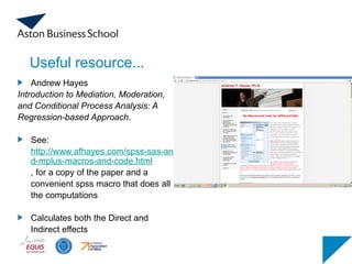
Useful resource...
Andrew Hayes
Introduction to Mediation, Moderation,
and Conditional Process Analysis: A
Regression-based Approach.
See:
http://www.afhayes.com/spss-sas-an
d-mplus-macros-and-code.html
, for a copy of the paper and a
convenient spss macro that does all
the computations
Calculates both the Direct and
Indirect effects

Moderator
A moderator “partitions a focal [independent] variable into
subgroups that establish its domains of maximal effectiveness in
regard to a given dependent variable” (Baron and Kenny, 1986).
Independent
Variable
Moderator
Dependent
Variable

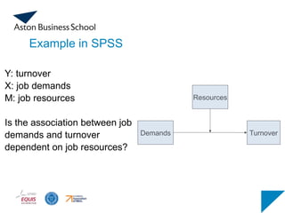
Example in SPSS
Y: turnover
X: job demands
M: job resources
Is the association between job
demands and turnover
dependent on job resources?
Demands
Resources
Turnover

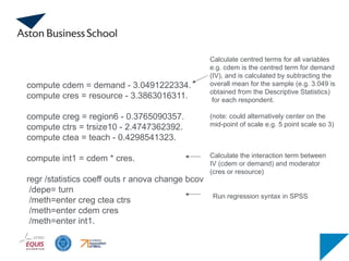
compute cdem = demand - 3.0491222334.
compute cres = resource - 3.3863016311.
compute creg = region6 - 0.3765090357.
compute ctrs = trsize10 - 2.4747362392.
compute ctea = teach - 0.4298541323.
compute int1 = cdem * cres.
regr /statistics coeff outs r anova change bcov
/depe= turn
/meth=enter creg ctea ctrs
/meth=enter cdem cres
/meth=enter int1.
Calculate centred terms for all variables
e.g. cdem is the centred term for demand
(IV), and is calculated by subtracting the
overall mean for the sample (e.g. 3.049 is
obtained from the Descriptive Statistics)
for each respondent.
(note: could alternatively center on the
mid-point of scale e.g. 5 point scale so 3)
Calculate the interaction term between
IV (cdem or demand) and moderator
(cres or resource)
Run regression syntax in SPSS

)
(
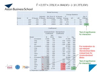
357
.
11
)
(
)
(
864
.
)
(
335
.
537
.
2
ˆ XM
M
X
Y 




For moderation do
not interpret
Standardised Beta
instead look for
Unstandardized
Betas
Test of significance
for interaction
Model Summary
Model R R Square
Adjusted
R Square
Std. Error of
the Estimate
Change Statistics
R Square
Change
F
Change df1 df2
Sig. F
Change
1 .484a
.234 .220 .51952 .234 16.381 3 161 .000
2 .493b
.243 .219 .51961 .009 .973 2 159 .380
3 .534c
.285 .258 .50663 .042 9.252 1 158 .003
Coefficientsa
Model
Unstandardized
Coefficients
Standardized
Coefficients
t Sig.
B
Std.
Error Beta
1 (Constant) 2.635 .064 41.054 .000
creg .649 .110 .416 5.919 .000
ctea .096 .110 .070 .867 .387
ctrs -.055 .019 -.229 -2.856 .005
2 (Constant) 2.606 .069 37.884 .000
creg .622 .114 .398 5.467 .000
ctea .060 .115 .044 .519 .604
ctrs -.045 .020 -.191 -2.229 .027
cdem .262 .459 .049 .571 .569
cres .877 .633 .125 1.385 .168
3 (Constant) 2.537 .071 35.835 .000
creg .537 .114 .344 4.694 .000
ctea .080 .113 .059 .714 .476
ctrs -.048 .020 -.201 -2.404 .017
cdem .335 .448 .062 .748 .456
cres .864 .617 .123 1.401 .163
int1 -11.357 3.734 -.213 -3.042 .003
a. Dependent Variable: turn
b0
b1
b2
b3
Test of significance
for interaction

Plotting the interaction
To interpret moderation results, use an Excel file to plot the
graphs (available at www.jeremydawson.co.uk/slopes.htm)
Follows procedure suggested by Aiken and West (1991)
need to calculate values for high (+1SD) and low (-1SD) X as
a function of high (+1SD) and low (-1SD) values on the
moderator M
The Excel file can also be used to test whether single slopes are
significant.

Adapted from Dawson, 2006
For further information on Excel sheets
see: www.jeremydawson.co.uk/slopes.htm

Moderated
Mediation/Mediated
Moderation

Integrating Mediation and Moderation
Edwards, J. R., & Lambert, L. S. (2007). Methods for integrating
moderation and mediation: A general analytical framework using
moderated path analysis. Psychological Methods, 12, 1-22.
www.afhayes.com/spss-sas-and-mplus-macros-and-code.html
Independent
Variable
Mediator
Dependent
Variable
Moderator

References
Field, A. (2009). Discovering statistics using SPSS. Sage.
Chapter 2 (Statistical Models)
Chapter 7 (Correlation)
Chapter 8 (Regression)
Chapter 9 (t-test)
Chapter 11 (ANOVA)
Chapter 10 (Moderation and Mediation)
Dawson, J.F. (2014). Moderation in Management Research:
What, Why, When and How. Journal of Business Psychology, 29,
1-19.

Courses_Advanced Statistics (14-15).pptx

More Related Content

Similar to Courses_Advanced Statistics (14-15).pptx

More from AstirLe

Recently uploaded

Courses_Advanced Statistics (14-15).pptx