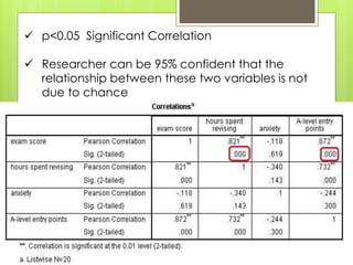
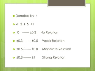
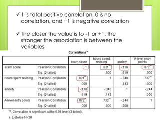
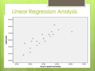
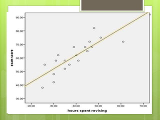
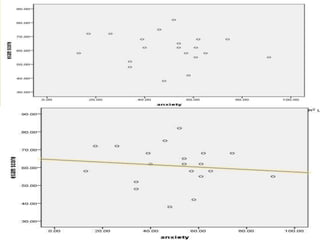
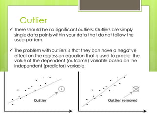
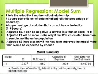
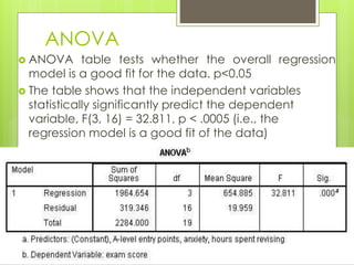
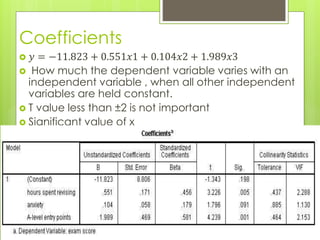
NYC Charter
School
Performance on
the 2012-13 State
Exams

1.

Bivariate
Correlations

2.

Linear Regression
Analysis

3.

Multiple
Regression
Analysis
Bivariate Correlations
 Bivariate

Correlation

 Paersone

Correlation or Co-efficient of
correlation

 Scale

level of measurement
 p<0.05 Significant Correlation
 Researcher can be 95% confident that the
relationship between these two variables is not
due to chance
 Denoted
 -1

by r

≤ r ≤ +1



0 ------- ±0.3

No Relation



±0.3 ------- ±0.5

Weak Relation



±0.5 ------- ±0.8

Moderate Relation



±0.8 ------- ±1

Strong Relation
 1 is total positive correlation, 0 is no
correlation, and −1 is negative correlation

 The closer the value is to -1 or +1, the
stronger the association is between the
variables
Linear Regression Analysis
Outlier
 There should be no significant outliers. Outliers are simply
single data points within your data that do not follow the
usual pattern.
 The problem with outliers is that they can have a negative
effect on the regression equation that is used to predict the
value of the dependent (outcome) variable based on the
independent (predictor) variable.
Multiple Regression: Model Sum

a. R tells the reliability & mathematical relationship.
1. R Square (co-efficient of determination) tells the percentage of
accuracy.
2. Also percentage of variation that can not be controlled i.e.
3. (1-R Square)
i.
Adjusted R2, It can be negative & always less than or equal to R
ii. Adjusted R2 will be more useful only if the R2 is calculated based on
a sample, not the entire population
iii. Adjusted R2 increases only if the new term improves the model more
than would be expected by chance
ANOVA
 ANOVA

table tests whether the overall regression
model is a good fit for the data. p<0.05
 The table shows that the independent variables
statistically significantly predict the dependent
variable, F(3, 16) = 32.811, p < .0005 (i.e., the
regression model is a good fit of the data)
Coefficients
𝑦 = −11.823 + 0.551𝑥1 + 0.104𝑥2 + 1.989𝑥3
 How much the dependent variable varies with an
independent variable , when all other independent
variables are held constant.
 T value less than ±2 is not important
 Significant value of x


Correlation & Linear Regression

  • 1.
    NYC Charter School Performance on the2012-13 State Exams 1. Bivariate Correlations 2. Linear Regression Analysis 3. Multiple Regression Analysis
  • 2.
    Bivariate Correlations  Bivariate Correlation Paersone Correlation or Co-efficient of correlation  Scale level of measurement
  • 3.
     p<0.05 SignificantCorrelation  Researcher can be 95% confident that the relationship between these two variables is not due to chance
  • 4.
     Denoted  -1 byr ≤ r ≤ +1  0 ------- ±0.3 No Relation  ±0.3 ------- ±0.5 Weak Relation  ±0.5 ------- ±0.8 Moderate Relation  ±0.8 ------- ±1 Strong Relation
  • 5.
     1 istotal positive correlation, 0 is no correlation, and −1 is negative correlation  The closer the value is to -1 or +1, the stronger the association is between the variables
  • 6.
  • 9.
    Outlier  There shouldbe no significant outliers. Outliers are simply single data points within your data that do not follow the usual pattern.  The problem with outliers is that they can have a negative effect on the regression equation that is used to predict the value of the dependent (outcome) variable based on the independent (predictor) variable.
  • 10.
    Multiple Regression: ModelSum a. R tells the reliability & mathematical relationship. 1. R Square (co-efficient of determination) tells the percentage of accuracy. 2. Also percentage of variation that can not be controlled i.e. 3. (1-R Square) i. Adjusted R2, It can be negative & always less than or equal to R ii. Adjusted R2 will be more useful only if the R2 is calculated based on a sample, not the entire population iii. Adjusted R2 increases only if the new term improves the model more than would be expected by chance
  • 11.
    ANOVA  ANOVA table testswhether the overall regression model is a good fit for the data. p<0.05  The table shows that the independent variables statistically significantly predict the dependent variable, F(3, 16) = 32.811, p < .0005 (i.e., the regression model is a good fit of the data)
  • 12.
    Coefficients 𝑦 = −11.823+ 0.551𝑥1 + 0.104𝑥2 + 1.989𝑥3  How much the dependent variable varies with an independent variable , when all other independent variables are held constant.  T value less than ±2 is not important  Significant value of x 