deep learning

1. Deep Learning
Convolutional and Pooling Layers
Dr. Ahsen Tahir
.The slides in part have been modified from Ian Good Fellow book slides and Alex’s Dive in to Deep Learning book slides

2. Convolutional Networks

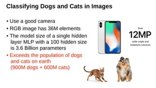
3. Classifying Dogs and Cats in Images
• Use a good camera
• RGB image has 36M elements
• The model size of a single hidden
layer MLP with a 100 hidden size
is 3.6 Billion parameters
• Exceeds the population of dogs
and cats on earth
(900M dogs + 600M cats)

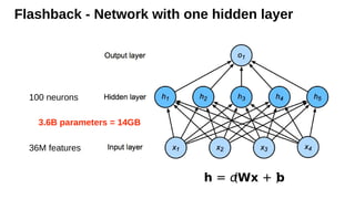
4. Flashback - Network with one hidden layer
36M features
100 neurons
h = σ
(Wx + b
)
3.6B parameters = 14GB

8. Convolution

10. 2-D Convolution (Cross Correlation)
(vdumoulin@ Github)
0 × 0 + 1 × 1 + 3 × 2 + 4 × 3 = 19,
1 × 0 + 2 × 1 + 4 × 2 + 5 × 3 = 25,
3 × 0 + 4 × 1 + 6 × 2 + 7 × 3 = 37,
4 × 0 + 5 × 1 + 7 × 2 + 8 × 3 = 43.

15. • Translation
Invariance
• Locality
Two Principles

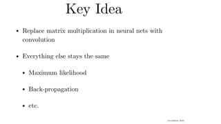
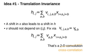
16. Idea #1 - Translation Invariance
• A shift in x also leads to a shift in h
• v should not depend on (i,j). Fix via vi, j,a,b= v
a,b
hi, j=∑
a,b
va,b
xi+a,j+b
hi, j=∑
a,b
vi, j,a,b
xi+a,j+b
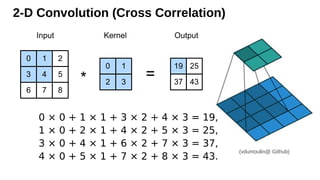
That’s a 2-D convolution
cross-correlation

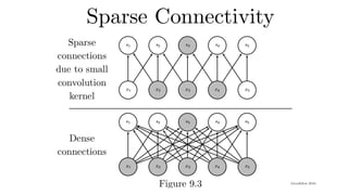
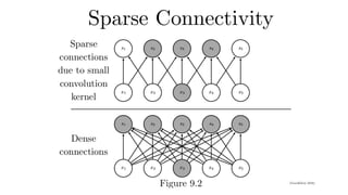
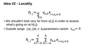
17. Idea #2 - Locality
• We shouldn’t look very far from x(i,j) in order to assess
what’s going on at h(i,j)
• Outside range parameters vanish
hi, j=
∑
a,b
va,bxi+a,j+b
|a|,|b| > Δ va,b= 0
hi, j=
Δ
∑
a=−Δ
Δ
∑
b=−Δ
va,b xi+a,j+b

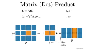
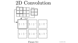
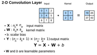
18. 2-D Convolution Layer
• input matrix
• kernel matrix
• b: scalar bias
• output matrix
• W and b are learnable parameters
Y = X ⋆ W + b
X : nh
× nw
W : kh
× kw
Y : (n
h
− kh
+ 1) × (n
w
− k
w
+ 1)

19. Examples
Edge Detection
Sharpen
Gaussian Blur
(wikipedia)

20. Examples
(Rob Fergus)

21. Gabor filters
@medium

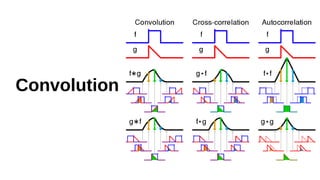
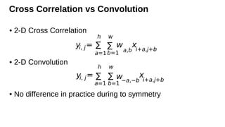
24. Cross Correlation vs Convolution
• 2-D Cross Correlation
• 2-D Convolution
• No difference in practice during to symmetry
yi, j=
h
∑
a=1
w
∑
b=1
w
a,b
xi+a,j+b
yi, j=
h
∑
a=1
w
∑
b=1
w−a,−b
x
i+a,j+b

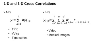
25. 1-D and 3-D Cross Correlations
yi =
h
∑
a=1
waxi+a yi, j,k=
h
∑
a=1
w
∑
b=1
d
∑
c=1
w
a,b,c
x
i+a,j+b,k+c
• 1-D
• Text
• Voice
• Time series
• 3-D
• Video
• Medical images

26. courses.d2l.ai/berkeley-stat-157
Padding and Stride

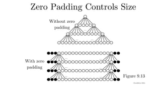
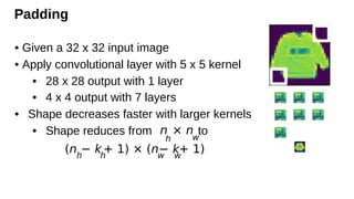
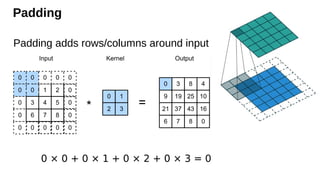
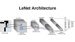
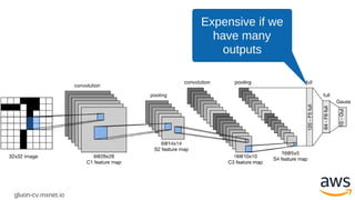
28. Padding
• Given a 32 x 32 input image
• Apply convolutional layer with 5 x 5 kernel
• 28 x 28 output with 1 layer
• 4 x 4 output with 7 layers
• Shape decreases faster with larger kernels
• Shape reduces from to
n
h
× n
w
(nh
− kh
+ 1) × (nw
− k
w
+ 1)

29. Padding
Padding adds rows/columns around input
0 × 0 + 0 × 1 + 0 × 2 + 0 × 3 = 0

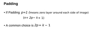
30. Padding
• If Padding
• A common choice is
(n − k
+ 2p + 1)
p=1 (means zero layer around each side of image)
2p= k − 1

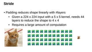
31. Stride
• Padding reduces shape linearly with #layers
• Given a 224 x 224 input with a 5 x 5 kernel, needs 44
layers to reduce the shape to 4 x 4
• Requires a large amount of computation

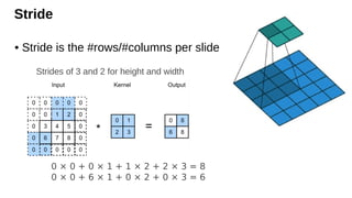
32. Stride
• Stride is the #rows/#columns per slide
Strides of 3 and 2 for height and width
0 × 0 + 0 × 1 + 1 × 2 + 2 × 3 = 8
0 × 0 + 6 × 1 + 0 × 2 + 0 × 3 = 6

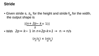
33. Stride
• Given stride s, for the height and stride for the width,
the output shape is
• With
sh
sw
2p= k− 1 in n+2p-k+1 → n → n/s
(n
h
/s
h
) × (n
w
/s
w
)
(n − k+ 1)
+ 2p
s
⌊ ⌋

34. courses.d2l.ai/berkeley-stat-157
Multiple Input and
Output Channels

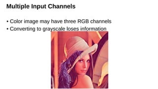
35. Multiple Input Channels
• Color image may have three RGB channels
• Converting to grayscale loses information

36. Multiple Input Channels
• Color image may have three RGB channels
• Converting to grayscale loses information

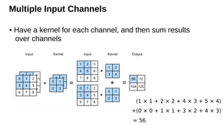
37. Multiple Input Channels
• Have a kernel for each channel, and then sum results
over channels
(1 × 1 + 2 × 2 + 4 × 3 + 5 × 4)
+(0 × 0 + 1 × 1 + 3 × 2 + 4 × 3)
= 56

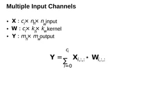
38. Multiple Input Channels
• input
• kernel
• output
X : ci
× nh
× nw
W : ci
× kh
× kw
Y : mh
× mw
Y =
ci
∑
i=0
Xi,:,:⋆ Wi,:,:

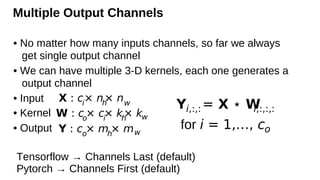
39. Multiple Output Channels
• No matter how many inputs channels, so far we always
get single output channel
• We can have multiple 3-D kernels, each one generates a
output channel
• Input
• Kernel
• Output
X : ci
× nh
× nw
W : co
× ci
× kh
× kw
Y : co
× mh
× mw
Yi,:,:= X ⋆ W
i,:,:,:
for i = 1,…, co
Tensorflow → Channels Last (default)
Pytorch → Channels First (default)

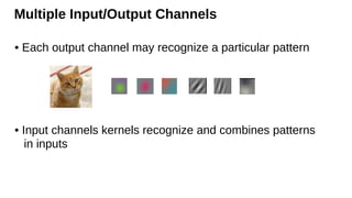
40. Multiple Input/Output Channels
• Each output channel may recognize a particular pattern
• Input channels kernels recognize and combines patterns
in inputs

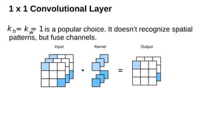
41. 1 x 1 Convolutional Layer
is a popular choice. It doesn’t recognize spatial
patterns, but fuse channels.
kh= kw
= 1

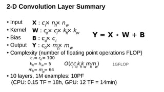
42. 2-D Convolution Layer Summary
• Input
• Kernel
• Bias
• Output
• Complexity (number of floating point operations FLOP)
• 10 layers, 1M examples: 10PF
(CPU: 0.15 TF = 18h, GPU: 12 TF = 14min)
X : ci
× nh
× nw
W : co
× ci
× kh
× kw
Y : co× mh
× mw
Y = X ⋆ W + B
B : co
× ci
O(c
i
c
o
k
h
k
w
m
h
m
w
)
ci = co= 100
kh= hw= 5
mh= mw
= 64
1GFLOP

43. courses.d2l.ai/berkeley-stat-157
Pooling Layer

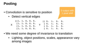
44. Pooling
• Convolution is sensitive to position
• Detect vertical edges
• We need some degree of invariance to translation
• Lighting, object positions, scales, appearance vary
among images
X Y
0 output with
1 pixel shift

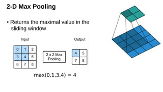
45. 2-D Max Pooling
• Returns the maximal value in the
sliding window
max(0,1,3,4) = 4

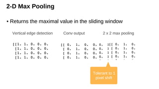
46. 2-D Max Pooling
• Returns the maximal value in the sliding window
Conv output 2 x 2 max pooling
Vertical edge detection
Tolerant to 1
pixel shift

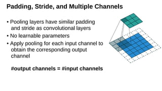
47. Padding, Stride, and Multiple Channels
• Pooling layers have similar padding
and stride as convolutional layers
• No learnable parameters
• Apply pooling for each input channel to
obtain the corresponding output
channel
#output channels = #input channels

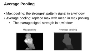
48. Average Pooling
• Max pooling: the strongest pattern signal in a window
• Average pooling: replace max with mean in max pooling
• The average signal strength in a window
Max pooling Average pooling

49. LeNet Architecture

50. courses.d2l.ai/berkeley-stat-157
Handwritten Digit
Recognition

51. courses.d2l.ai/berkeley-stat-157
MNIST
• Centered and scaled
• 50,000 training data
• 10,000 test data
• 28 x 28 images
• 10 classes

52. courses.d2l.ai/berkeley-stat-157
Y. LeCun, L.
Bottou, Y. Bengio,
P. Haffner, 1998
Gradient-based
learning applied to
document
recognition

53. courses.d2l.ai/berkeley-stat-157
Y. LeCun, L.
Bottou, Y. Bengio,
P. Haffner, 1998
Gradient-based
learning applied to
document
recognition

54. gluon-cv.mxnet.io
Expensive if we
have many
outputs

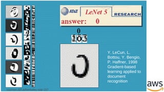
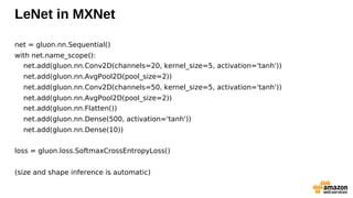
55. LeNet in MXNet
net = gluon.nn.Sequential()
with net.name_scope():
net.add(gluon.nn.Conv2D(channels=20, kernel_size=5, activation='tanh'))
net.add(gluon.nn.AvgPool2D(pool_size=2))
net.add(gluon.nn.Conv2D(channels=50, kernel_size=5, activation='tanh'))
net.add(gluon.nn.AvgPool2D(pool_size=2))
net.add(gluon.nn.Flatten())
net.add(gluon.nn.Dense(500, activation='tanh'))
net.add(gluon.nn.Dense(10))
loss = gluon.loss.SoftmaxCrossEntropyLoss()
(size and shape inference is automatic)

56. courses.d2l.ai/berkeley-stat-157
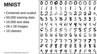
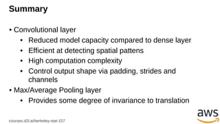
Summary
• Convolutional layer
• Reduced model capacity compared to dense layer
• Efficient at detecting spatial pattens
• High computation complexity
• Control output shape via padding, strides and
channels
• Max/Average Pooling layer
• Provides some degree of invariance to translation