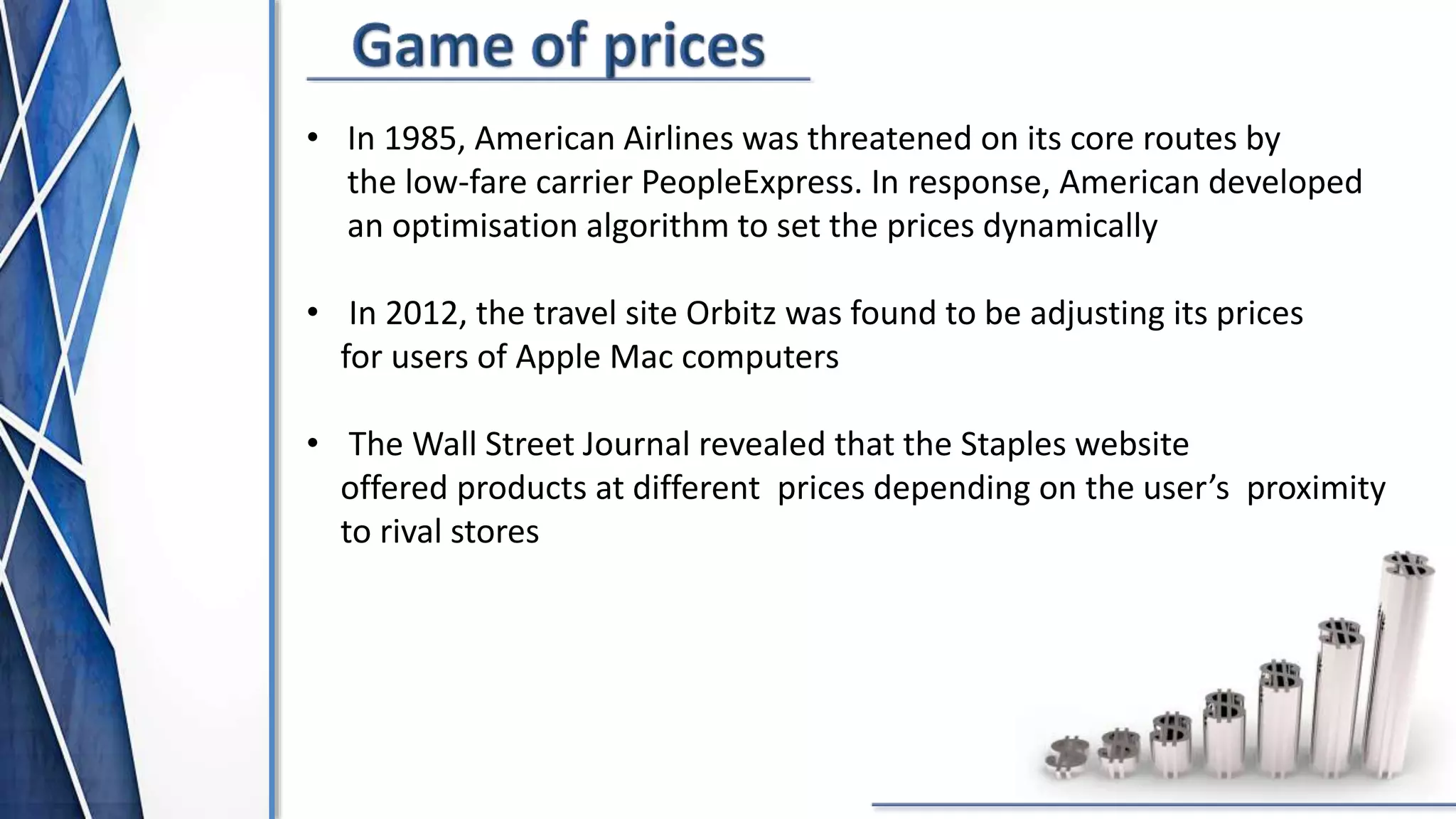
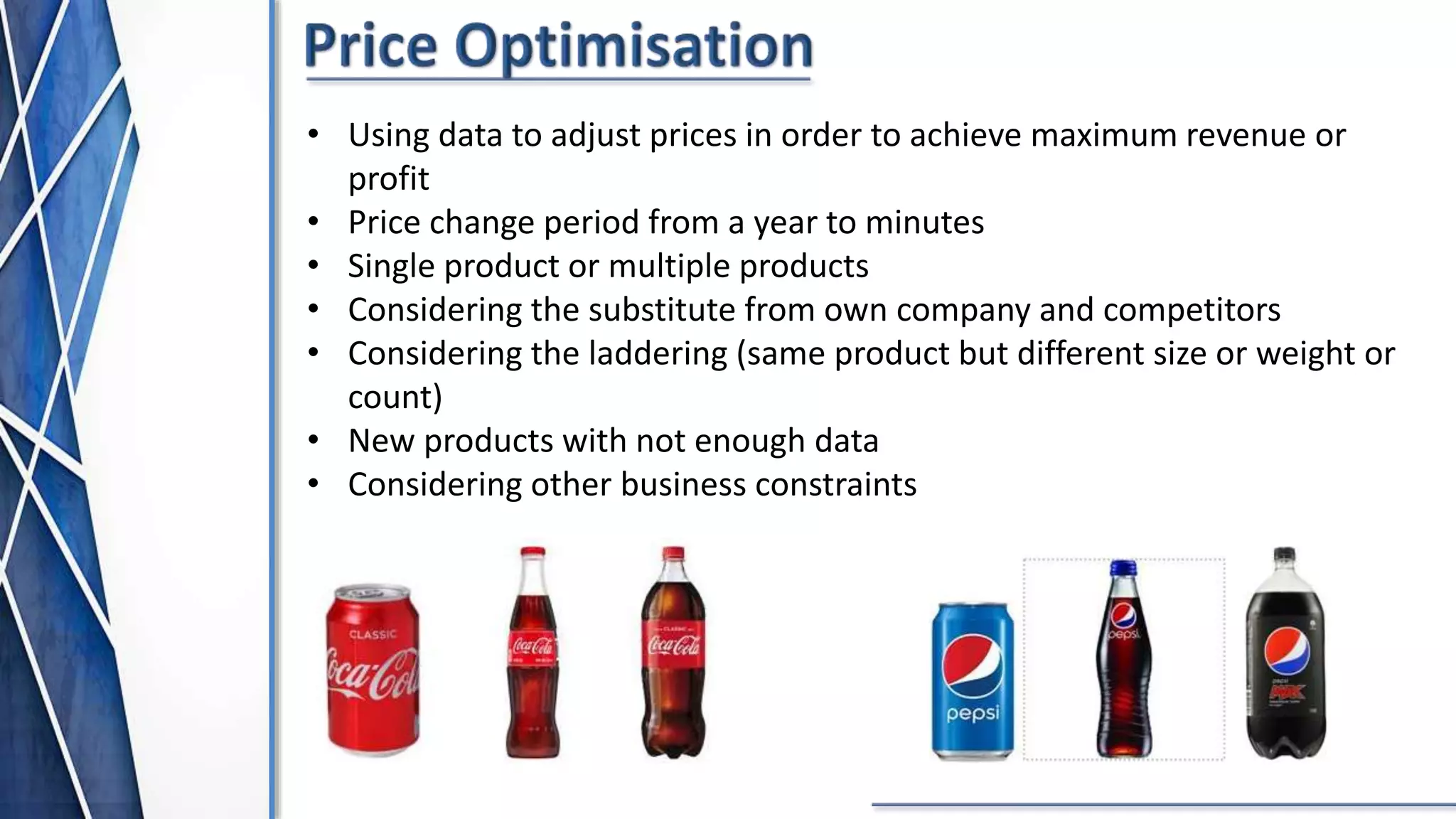
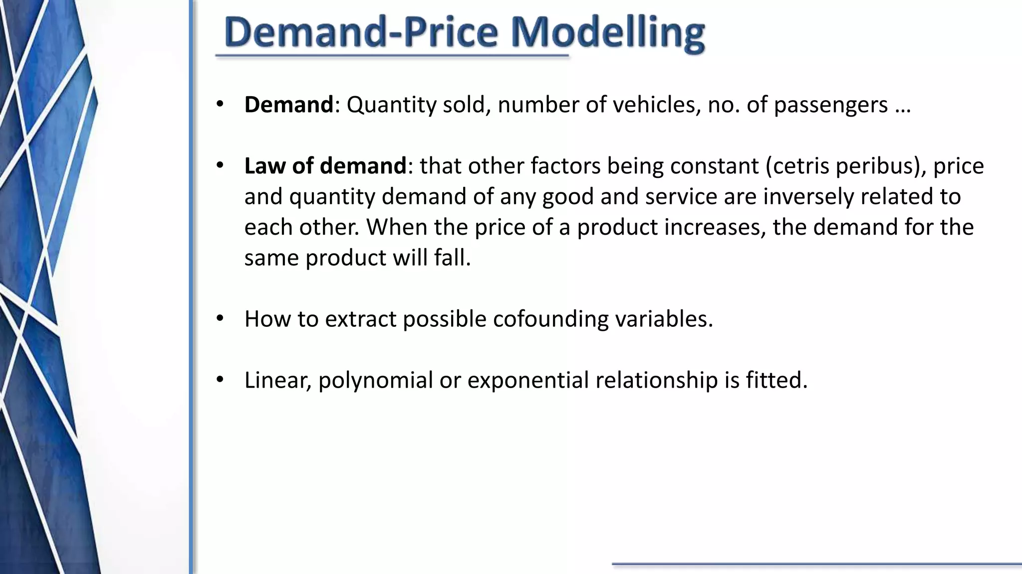
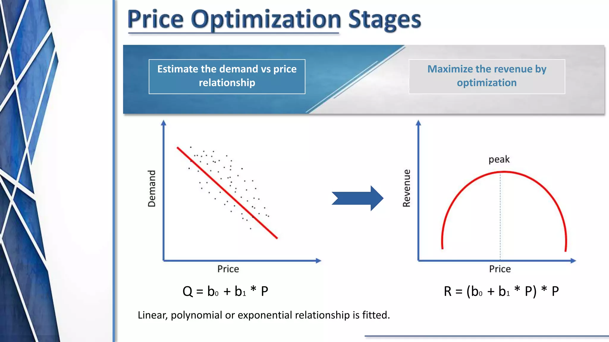
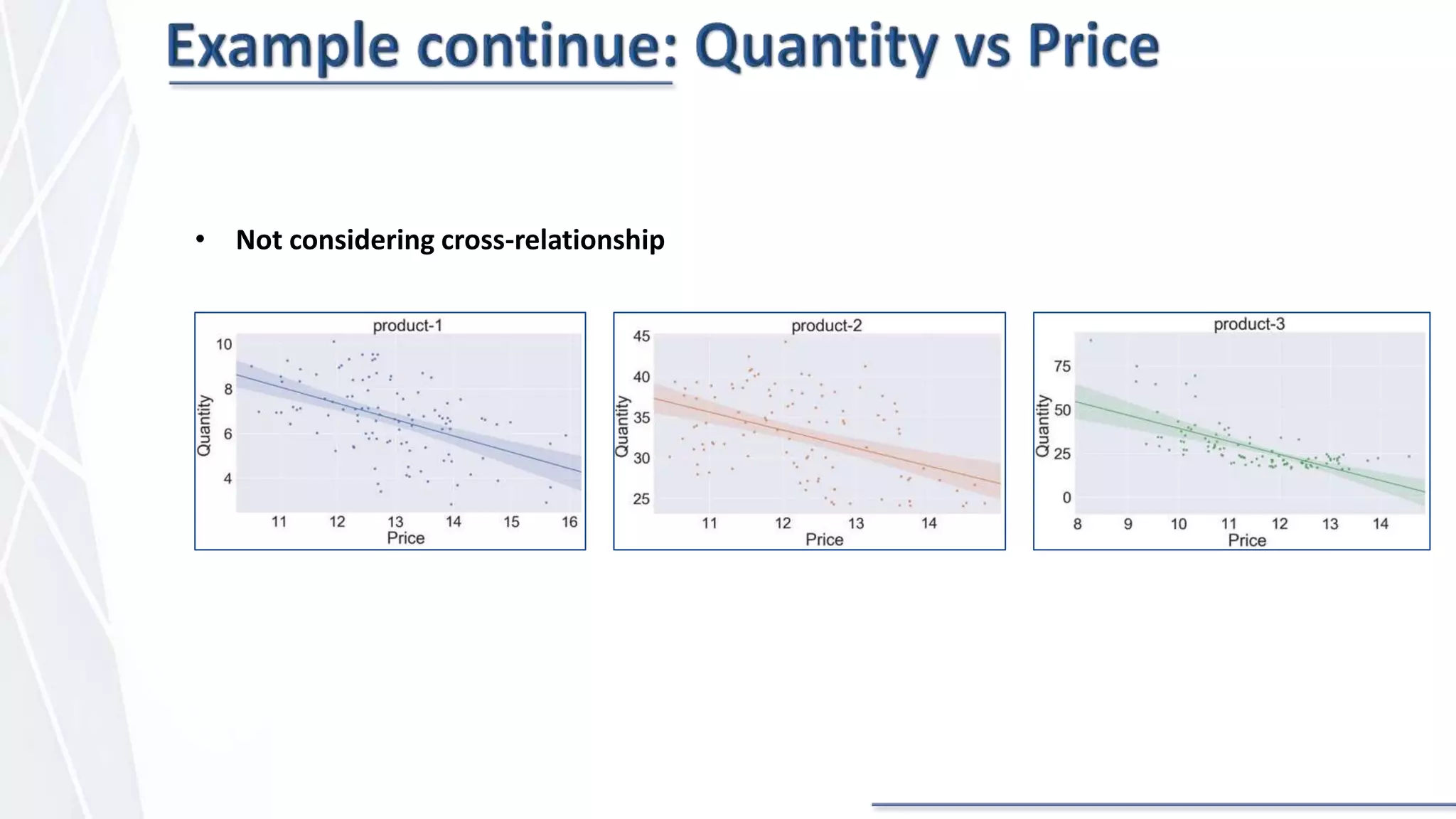
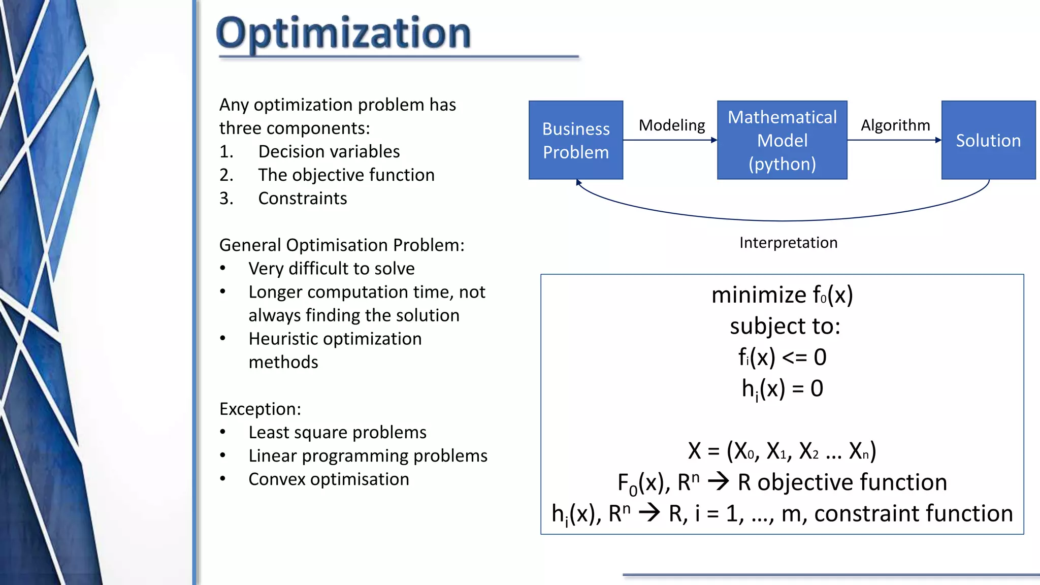
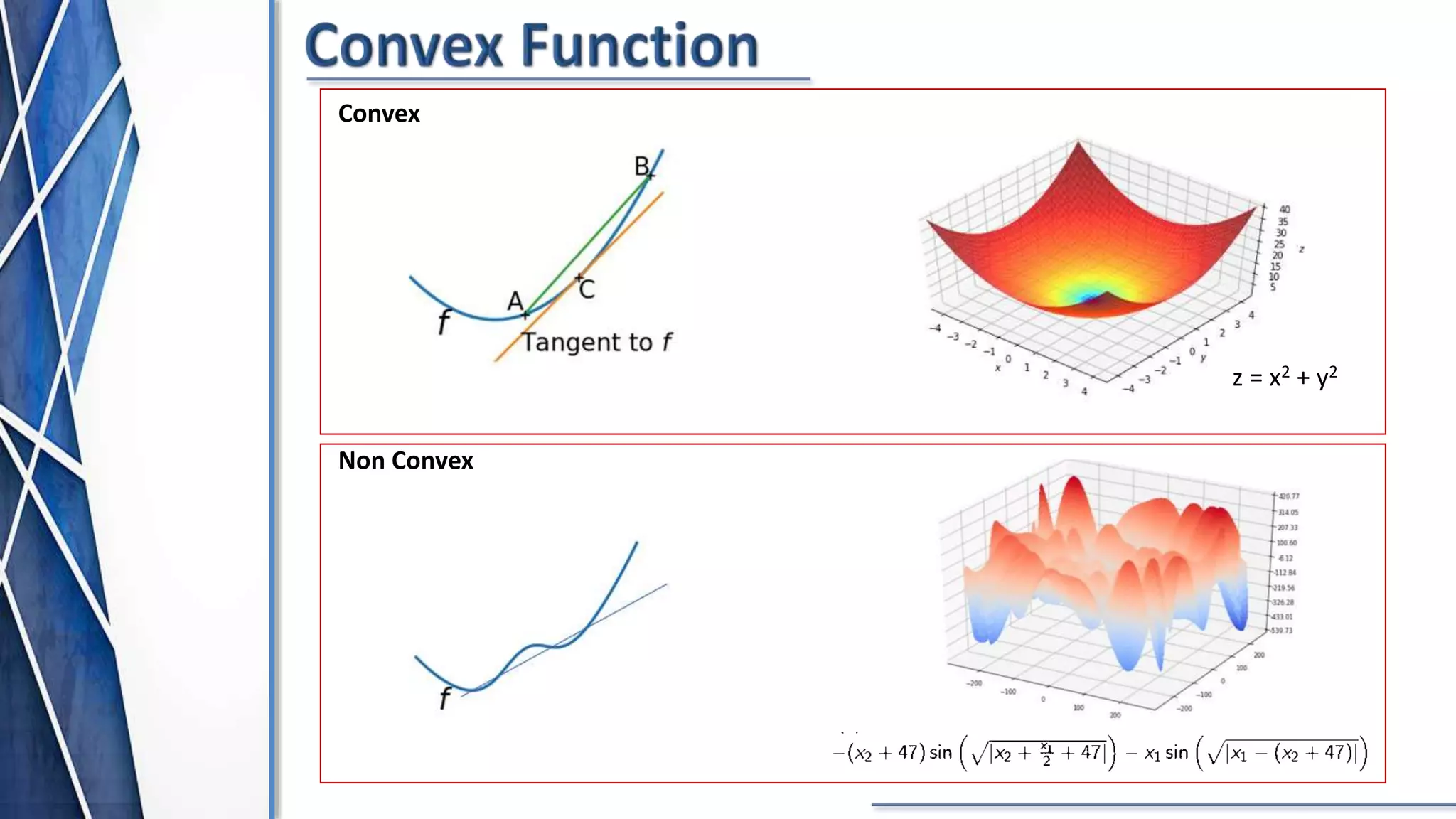
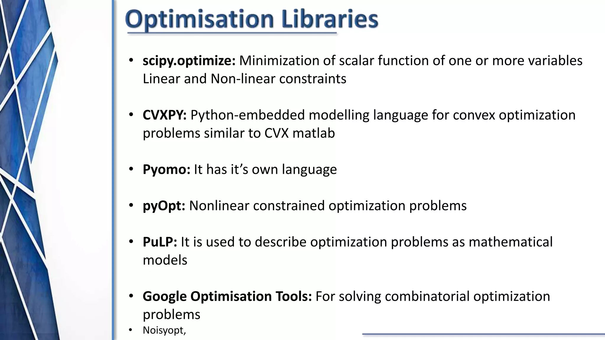
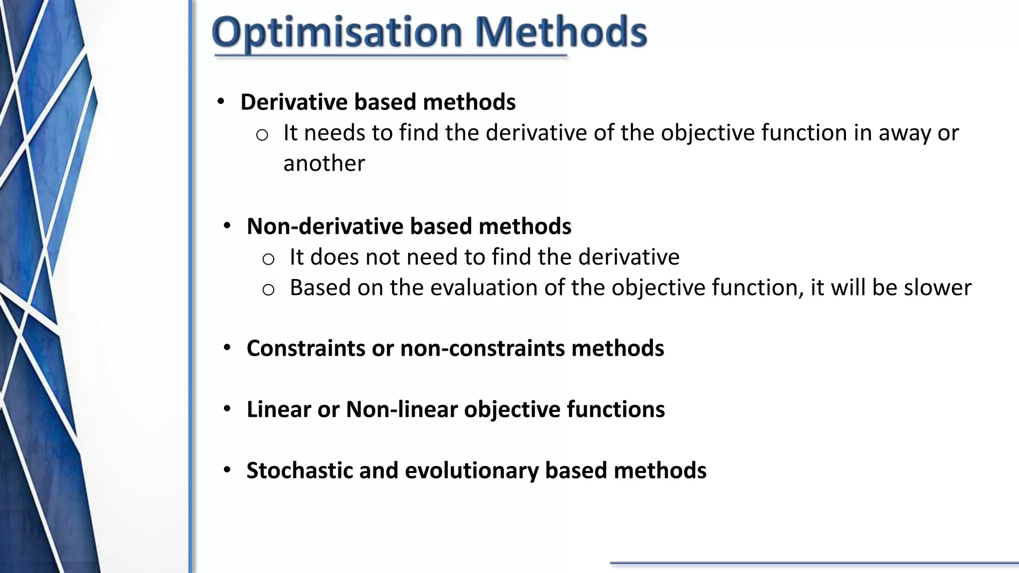
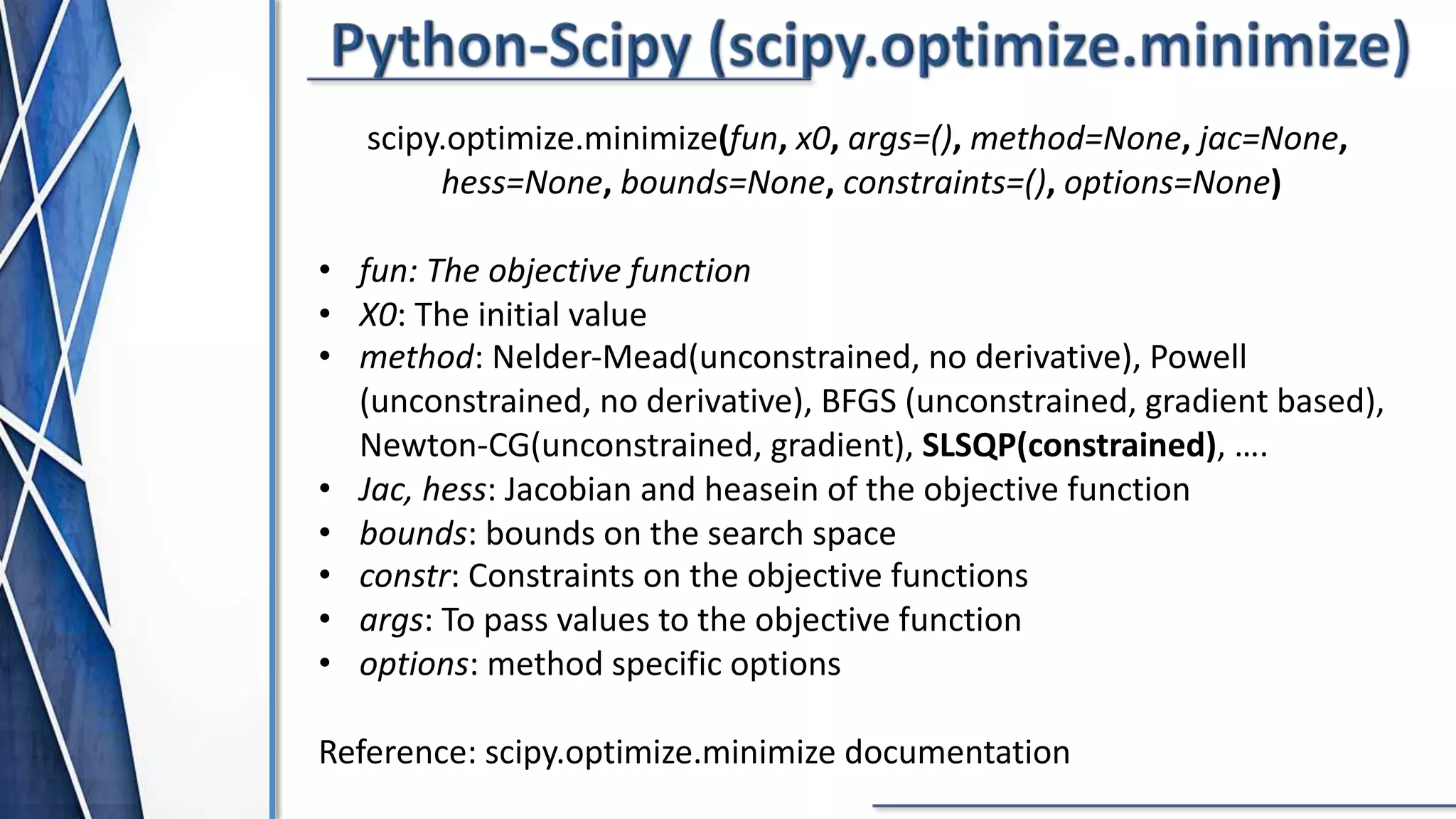
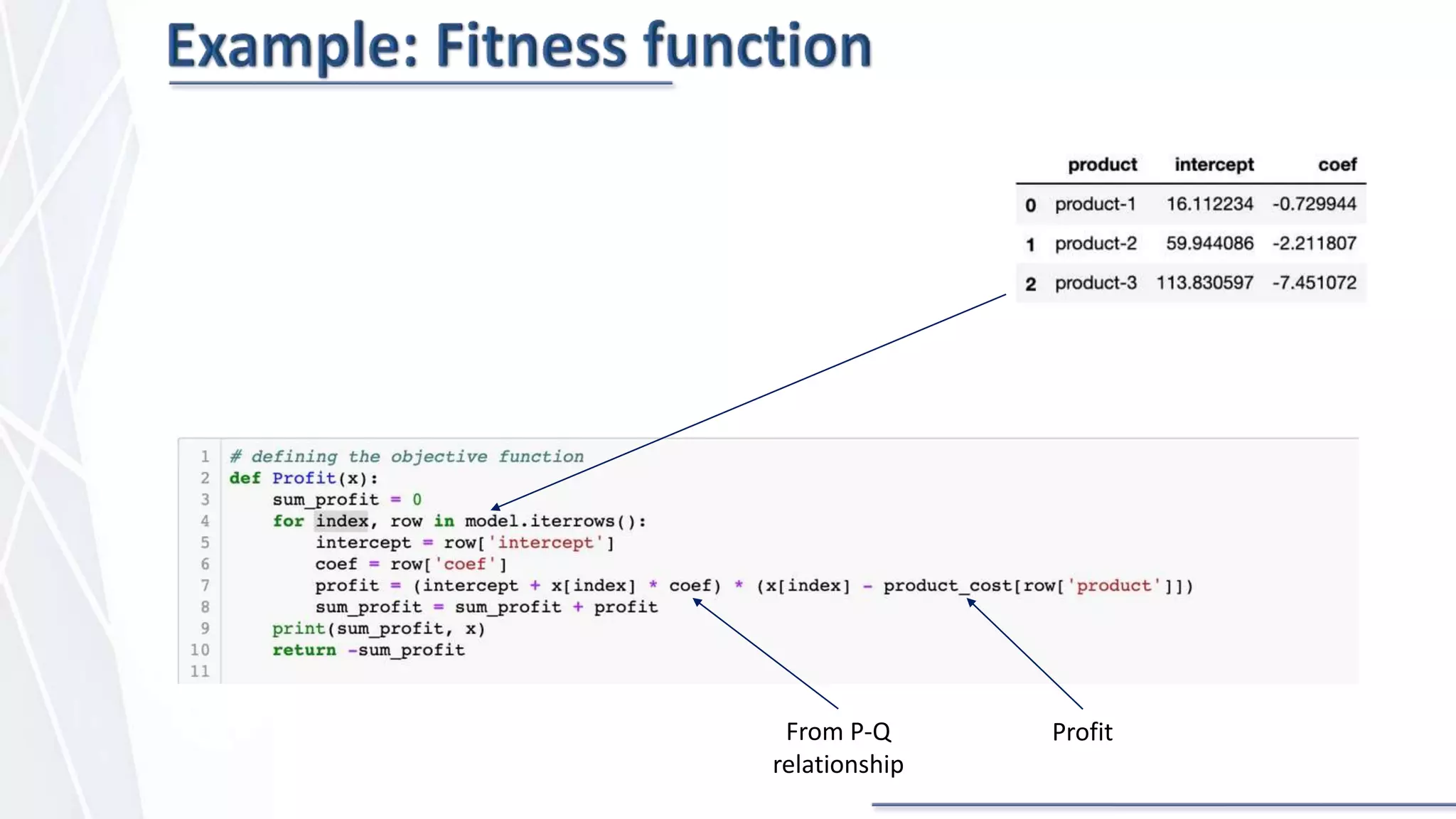
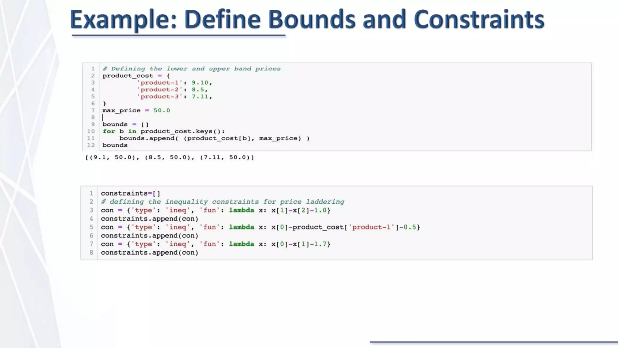
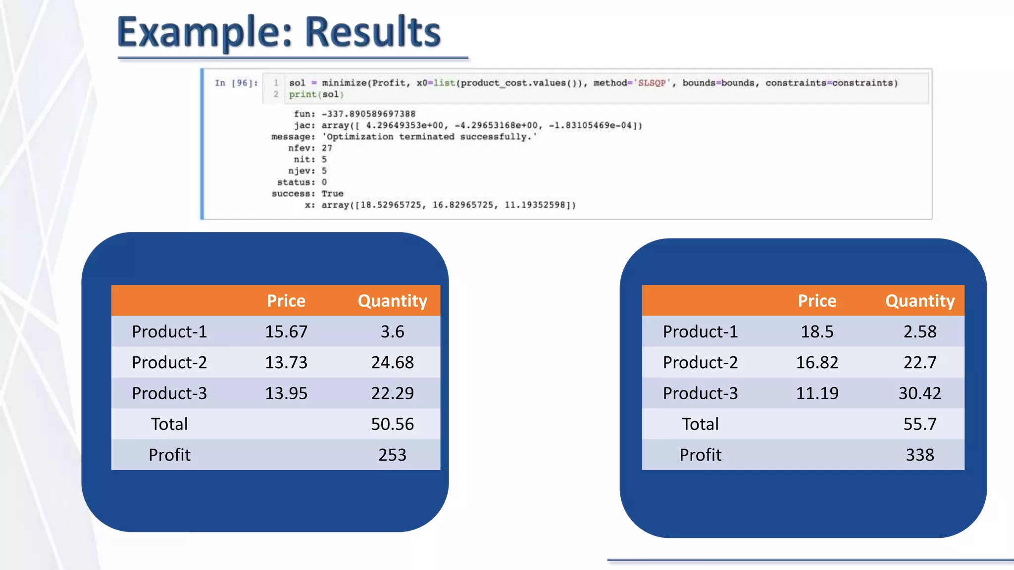
The document discusses price optimization with Python. It describes how companies like American Airlines and Orbitz have used algorithms to dynamically set prices. The key aspects of price optimization are discussed, including maximizing revenue by estimating demand curves and fitting relationships. Different optimization techniques in Python are also covered, such as scipy.optimize and constraint methods like SLSQP. Overall the document provides an overview of using Python for price optimization problems.

1. Price Optimisation with Python
Ammar Mohemmed
21/07/2019

2. • In 1985, American Airlines was threatened on its core routes by
the low-fare carrier PeopleExpress. In response, American developed
an optimisation algorithm to set the prices dynamically
• In 2012, the travel site Orbitz was found to be adjusting its prices
for users of Apple Mac computers
• The Wall Street Journal revealed that the Staples website
offered products at different prices depending on the user’s proximity
to rival stores

3. • Using data to adjust prices in order to achieve maximum revenue or
profit
• Price change period from a year to minutes
• Single product or multiple products
• Considering the substitute from own company and competitors
• Considering the laddering (same product but different size or weight or
count)
• New products with not enough data
• Considering other business constraints

4. • Demand: Quantity sold, number of vehicles, no. of passengers …
• Law of demand: that other factors being constant (cetris peribus), price
and quantity demand of any good and service are inversely related to
each other. When the price of a product increases, the demand for the
same product will fall.
• How to extract possible cofounding variables.
• Linear, polynomial or exponential relationship is fitted.

5. Estimate the demand vs price
relationship
Maximize the revenue by
optimization
Q = b0 + b1 * P R = (b0 + b1 * P) * P
Linear, polynomial or exponential relationship is fitted.

6. • Is a phenomenon in probability and statistics, in which a trend appears
in several different groups of data but disappears or reverses when
these groups are combined (Wikipedia)

7. Quantity increases with price, but difference of quantity decreases
Quantity
Quantity vs. price Quantity difference vs. price
Quantity
difference

8. Objective function:
Profit – Q1*(P1-C1) + Q2*(P2-C2) + Q3*(P3-C3)
• Variables: P1, P2, P3
• Constraints:
 Product-2 price higher than Product-3 by 1
 Product-1 higher than its cost by 0.5
 Product-1 higher than product-2 by 1.7
• Bounds:
 Max price: 50
 Min price: product cost

9. • Not considering cross-relationship

10. Any optimization problem has
three components:
1. Decision variables
2. The objective function
3. Constraints
General Optimisation Problem:
• Very difficult to solve
• Longer computation time, not
always finding the solution
• Heuristic optimization
methods
Exception:
• Least square problems
• Linear programming problems
• Convex optimisation
Business
Problem
Mathematical
Model
(python)
Solution
Modeling Algorithm
Interpretation
minimize f0(x)
subject to:
fi(x) <= 0
hi(x) = 0
X = (X0, X1, X2 … Xn)
F0(x), Rn  R objective function
hi(x), Rn  R, i = 1, …, m, constraint function

11. Convex
Non Convex
z = x2 + y2

12. • Derivative: Measures the sensitivity to change of the function value
(output value) with respect to a change in it’s argument (input value).
• Gradient: is a multi-variable generalization of the derivative. Points in
the direction of greatest increase of a function.
• Jacobian matrix: The first derivative of a vector-values function.
• Hessian matrix: is a square matrix of second-order partial derivative of
a scalar-valued function.

13. • scipy.optimize: Minimization of scalar function of one or more variables
Linear and Non-linear constraints
• CVXPY: Python-embedded modelling language for convex optimization
problems similar to CVX matlab
• Pyomo: It has it’s own language
• pyOpt: Nonlinear constrained optimization problems
• PuLP: It is used to describe optimization problems as mathematical
models
• Google Optimisation Tools: For solving combinatorial optimization
problems
• Noisyopt,

14. • Derivative based methods
o It needs to find the derivative of the objective function in away or
another
• Non-derivative based methods
o It does not need to find the derivative
o Based on the evaluation of the objective function, it will be slower
• Constraints or non-constraints methods
• Linear or Non-linear objective functions
• Stochastic and evolutionary based methods

15. scipy.optimize.minimize(fun, x0, args=(), method=None, jac=None,
hess=None, bounds=None, constraints=(), options=None)
• fun: The objective function
• X0: The initial value
• method: Nelder-Mead(unconstrained, no derivative), Powell
(unconstrained, no derivative), BFGS (unconstrained, gradient based),
Newton-CG(unconstrained, gradient), SLSQP(constrained), ….
• Jac, hess: Jacobian and heasein of the objective function
• bounds: bounds on the search space
• constr: Constraints on the objective functions
• args: To pass values to the objective function
• options: method specific options
Reference: scipy.optimize.minimize documentation
scipy.optimize.minimize(fun, x0, args=(), method=None, jac=None,
hess=None, bounds=None, constraints=(), options=None)
• fun: The objective function
• X0: The initial value
• method: Nelder-Mead(unconstrained, no derivative), Powell
(unconstrained, no derivative), BFGS (unconstrained, gradient based),
Newton-CG(unconstrained, gradient), SLSQP(constrained), ….
• Jac, hess: Jacobian and heasein of the objective function
• bounds: bounds on the search space
• constr: Constraints on the objective functions
• args: To pass values to the objective function
• options: method specific options
Reference: scipy.optimize.minimize documentation

16. From P-Q
relationship
Profit

18. Price Quantity
Product-1 18.5 2.58
Product-2 16.82 22.7
Product-3 11.19 30.42
Total 55.7
Profit 338
Proposed Prices and Quantities
Price Quantity
Product-1 15.67 3.6
Product-2 13.73 24.68
Product-3 13.95 22.29
Total 50.56
Profit 253
Last Week Prices and Quantities

19. • Stochastic Gradient Optimization
• Bayesian optimization​
• ADAM optimization​
• Evolutionary strategies​
• Enforcement learning​
• ……….

20. Questions and Answers