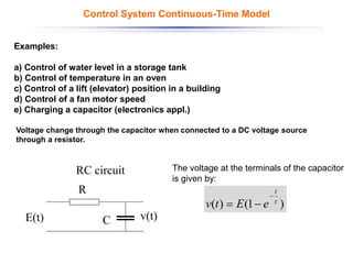
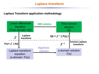
The document discusses control systems and their components, introducing block diagrams as a means to represent cause-and-effect relationships in dynamic systems. It explains the role of MATLAB and Simulink in modeling, simulation, and analysis, highlighting their utility in managing control system design and implementation. Furthermore, it details Laplace transforms as a mathematical tool for analyzing system behavior, providing methodologies for transforming time domain equations into the s-domain for easier solutions.
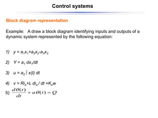
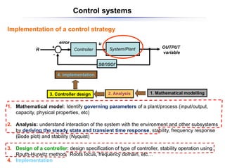
![Example 1. Generate a plot of 𝑦 𝑥 = 𝑒−0.7𝑥
sin(𝜔𝑥)
where ω = 15 rad/s, and 0<x<15. Use the colon notation to generate the x vector in increments
of 0.1.
Solution.
>> x = [0 : 0.1 : 15];
>> w = 15;
>> y = exp(– 0.7*x).*sin(w*x);
>> plot(x, y)
>> title(‘y(x) = e^-^0^.^7^x sinomega x’)
>> xlabel(‘x’)
>> ylabel(‘y)’](https://image.slidesharecdn.com/controlsystems-2-250112234421-b72a68f6/85/control-systems-block-representation-and-first-order-systems-9-320.jpg)
![t ≥ to
t < 0
0
)
(
=
= a
t
f
s
a
s
ae
dt
e
a
dt
e
t
f
t
f
L
st
st
st
=
−
=
=
=
−
−
−
0
0
0
)
(
)
(
)]
(
[
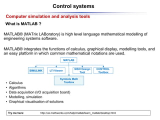
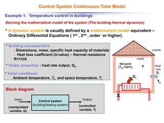
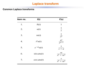
1) Step signal (Heaviside)
a
f(t)
t
f(t)
t
a
0
t
0
0
)]
(
[ 0
st
t
st
e
s
a
s
e
a
t
t
f
L −
−
=
−
=
−
−
=
=
0
st
dt
e
)
t
(
f
)
s
(
F
)]
t
(
f
[
L
L
2) Delayed step signal (Heaviside)
Laplace transform
Example of common signals
a
t
f =
)
(
L
L](https://image.slidesharecdn.com/controlsystems-2-250112234421-b72a68f6/85/control-systems-block-representation-and-first-order-systems-23-320.jpg)
![2
0
st
0
st
0
st
s
a
dt
e
s
a
s
ate
dt
ate
)]
t
(
r
[
L =
−
−
−
=
=
−
−
−
0
t
,
at
)
t
(
r
=
f(t)
t
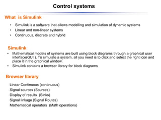
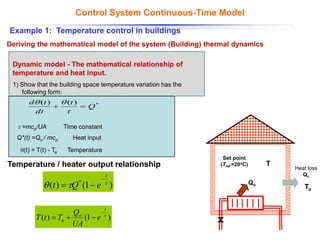
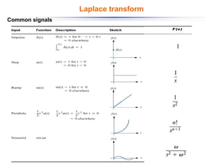
Laplace transform
Examples
3) Ramp signal
L
−
=
=
0
st
dt
e
)
t
(
f
)
s
(
F
)]
t
(
f
[
L
L](https://image.slidesharecdn.com/controlsystems-2-250112234421-b72a68f6/85/control-systems-block-representation-and-first-order-systems-24-320.jpg)
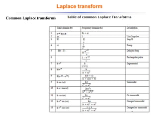
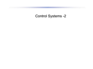
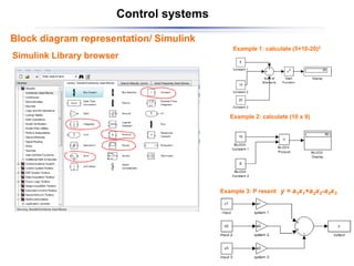
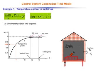
![Linearity properties of Laplace transform
)]
t
(
f
[
L
)
s
(
F 1
1 =
)]
t
(
f
[
L
)
s
(
F 2
2 =
ts
tan
Cons
c
,
c 2
1 =
)
(
.
)
(
.
)]
(
[
.
)]
(
[
.
)]
(
.
)
(
.
[
2
2
1
1
2
2
1
1
2
2
1
1
s
F
c
s
F
c
t
f
L
c
t
f
L
c
t
f
c
t
f
c
L
+
=
+
=
+
Laplace transform
L L L](https://image.slidesharecdn.com/controlsystems-2-250112234421-b72a68f6/85/control-systems-block-representation-and-first-order-systems-28-320.jpg)
![)
0
(
)
0
(
)
(
.
)]
(
[
]
[
)]
(
"
[ '
2
..
2
2
+
+
−
−
=
=
= f
sf
s
F
s
t
f
dt
f
d
t
f
Derivatives
)
0
(
f
)
s
(
F
.
s
)]
t
(
f
[
L
]
dt
df
[
L
)]
t
(
'
f
[
L +
•
−
=
=
=
)
1
(
)
1
(
2
1
)
0
(
.....
)
0
(
)
0
(
)
(
]
)
(
[
−
−
−
−
−
−
=
n
n
n
n
n
n
f
f
s
f
s
s
F
s
dt
t
df
)
1
i
(
n
1
i
i
n
n
)
n
(
)
0
(
f
.
s
)
s
(
F
s
]
)
t
(
f
[
L
−
=
−
−
=
Laplace transform
L L L
L L
L
L
L](https://image.slidesharecdn.com/controlsystems-2-250112234421-b72a68f6/85/control-systems-block-representation-and-first-order-systems-29-320.jpg)
![ =
t
0
s
)
s
(
F
]
du
)
u
(
f
[
L
Integral
Laplace transform
L](https://image.slidesharecdn.com/controlsystems-2-250112234421-b72a68f6/85/control-systems-block-representation-and-first-order-systems-30-320.jpg)