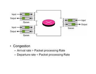
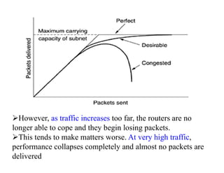
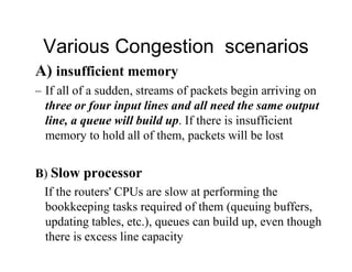
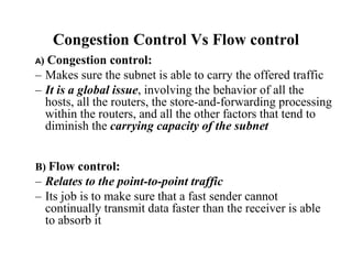
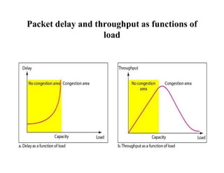
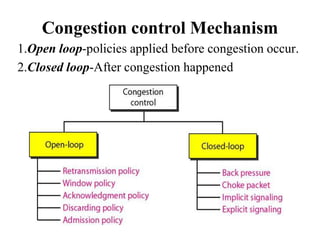
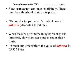
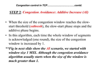
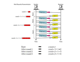
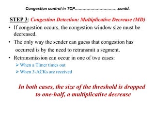
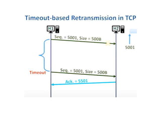
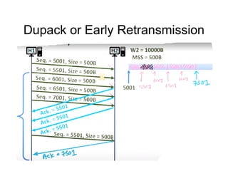
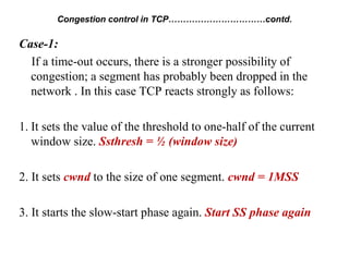
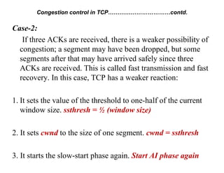
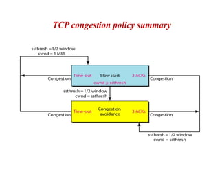
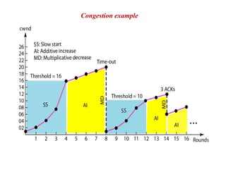
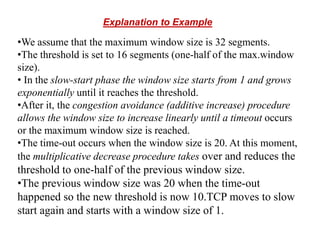
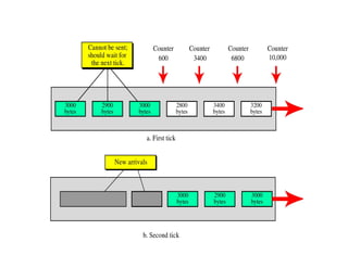
Top Rated Pune Call Girls Budhwar Peth ⟟ 6297143586 ⟟ Call Me For Genuine Se...
congestion control data communication.pdf
1. CONGESTION
• When too many packets are present in a part of the
network, performance degrades as router is not able
to clear up the traffic, this situation is called
congestion.
• congestion in a network may occur if the load on
the network (the number of packets sent to the
network) is greater than the capacity of the network
(the number of packets a network can handle)
2.
3. However, as traffic increases too far, the routers are no
longer able to cope and they begin losing packets.
This tends to make matters worse. At very high traffic,
performance collapses completely and almost no packets are
delivered
4. Various Congestion scenarios
A) insufficient memory
– If all of a sudden, streams of packets begin arriving on
three or four input lines and all need the same output
line, a queue will build up. If there is insufficient
memory to hold all of them, packets will be lost
B) Slow processor
If the routers' CPUs are slow at performing the
bookkeeping tasks required of them (queuing buffers,
updating tables, etc.), queues can build up, even though
there is excess line capacity
5. Congestion Control Vs Flow control
A) Congestion control:
– Makes sure the subnet is able to carry the offered traffic
– It is a global issue, involving the behavior of all the
hosts, all the routers, the store-and-forwarding processing
within the routers, and all the other factors that tend to
diminish the carrying capacity of the subnet
B) Flow control:
– Relates to the point-to-point traffic
– Its job is to make sure that a fast sender cannot
continually transmit data faster than the receiver is able
to absorb it
6. Congestion Control Vs Flow control…..contd..
• If Optical Network is there it can support
1000GBPS.
• A super computer generating the packets at a
rate 1Gbps, to a Personal computer in the
network ,
• In this case flow control will be required a
Network do not oppose the flow as it support
it,
• So Network do not have a congestion
problem.
9. General Principles of Congestion Control
(Open loop systems)
These systems are designed to minimize
congestion in the first place, rather than letting
it happen and reacting after the fact
Tools for implementing open-loop control
include deciding when to accept new traffic,
deciding when to discard packets and which
ones, and making scheduling decisions at
various points in the network
10. General Principles of Congestion Control
(Close loop systems)
Closed loop solutions are based on the concept of a
feedback loop
This approach has three parts when applied to
congestion control:
1)Monitor the system to detect when and where
congestion occurs
2)Pass this information to places where action
can be taken
3)Adjust system operation to correct the problem
11. General Principles of Congestion Control
(Close Loop systems)
Monitoring the system: A variety of metrics can be used to
monitor the subnet for congestion, among these are:
• The percentage of all packets discarded for lack of buffer
space
• The average queue lengths
• The number of packets that time out and are retransmitted
• The average packet delay
• The standard deviation of packet delay
In all cases, rising numbers indicate growing congestion.
12. General Principles of Congestion Control
(Close Loop systems)
The Feedback Loop: To transfer the information
about the congestion from the point where it is
detected to the point where something can be done
about it
1)One way is for the router detecting the congestion to send
a packet to the traffic source or sources, announcing the
problem
2)Other possibility is to send a bit or field reserved in every
packet for routers to fill in whenever congestion gets
above some threshold level
3)Third approach is to have hosts or routers periodically
send probe packets out to explicitly ask about congestion.
This information can then be used to route traffic around
problem areas
13. General Principles of Congestion Control
(Close Loop systems)
Adjust system operation :
Two possible solutions:
1)Increase the resources
2) Decrease the load
14. Closed loop methods
1.Back pressure: Congested node stops receiving
packets & inform the source to slow down,& increase
pressure on previous node & so on.
15. 2. Choke Packet : Congested node send a
choke packet directly to source, & ask him to
slow down or stop transmitting Packets
16. 3.Implicit signaling:
• There is no direct signaling between congested
node & source.
• The source suggest that there is congestion in
network by observing e.g that no ACK received
for many packets sent, & it slows down itself.
4.Explicit Signaling:
• Involves direct signaling between source &
congested node.
• However unlike choke packet no separate packet
is formed for this purpose. A bit in the packet
moving in forward/backward can be used as
warning bit.
17. Congestion control in TCP
• Sender window: Sender window size is determined by
two factors:
A) rwnd: Receiver window size (available buffer capacity
at receiver)
B) cwnd: Congestion window size (size determined by
network condition depending on current network
scenario and capabilities)
Sender window size = Min (rwnd, cwnd)
18. Congestion control in TCP……………………………contd.
In TCP congestion control take place in 3 steps:
STEP 1:Slow start (SS): Exponential Increase
• SS algorithm is based on the idea that the size of the
congestion window (cwnd) starts with one maximum
segment size (MSS).
• The MSS is determined during connection establishment
by using an option of the same name in TCP header.
• The size of the window increases one MSS each time an
acknowledgment is received.
• As the name implies, the window starts slowly, but grows
exponentially.
19. **Round refers to ACK of the whole
window segment
.
**in Fig 1 MSS =1 Byte and
Assumed that rwnd>cwnd and each
segment is ACK separately
20. • Slow start cannot continue indefinitely. There
must be a threshold to stop this phase.
• The sender keeps track of a variable named
ssthresh (slow-start threshold).
• When the size of window in bytes reaches this
threshold, slow start stops and the next phase
starts.
• In most implementations the value of ssthresh is
65,535 bytes.
Congestion control in TCP……………………………contd
21. STEP 2: Congestion Avoidance: Additive Increase (AI)
• When the size of the congestion window reaches the slow-
start threshold (ssthresh), the slow-start phase stops and the
additive phase begins.
• In this algorithm, each time the whole window of segments
is acknowledged (one round), the size of the congestion
window is increased by 1.
**Fig in next slide show the AI scenario, we started with
window size 1 MSS. Although the congestion avoidance
algorithm usually starts when the size of the window is
much greater than 1.
Congestion control in TCP……………………………contd.
22.
23. STEP 3: Congestion Detection: Multiplicative Decrease (MD)
• If congestion occurs, the congestion window size must be
decreased.
• The only way the sender can guess that congestion has
occurred is by the need to retransmit a segment.
• Retransmission can occur in one of two cases:
When a Timer times out
When 3-ACKs are received
In both cases, the size of the threshold is dropped
to one-half, a multiplicative decrease
Congestion control in TCP……………………………contd.
26. Case-1:
If a time-out occurs, there is a stronger possibility of
congestion; a segment has probably been dropped in the
network . In this case TCP reacts strongly as follows:
1. It sets the value of the threshold to one-half of the current
window size. Ssthresh = ½ (window size)
2. It sets cwnd to the size of one segment. cwnd = 1MSS
3. It starts the slow-start phase again. Start SS phase again
Congestion control in TCP……………………………contd.
27. Case-2:
If three ACKs are received, there is a weaker possibility of
congestion; a segment may have been dropped, but some
segments after that may have arrived safely since three
ACKs are received. This is called fast transmission and fast
recovery. In this case, TCP has a weaker reaction:
1. It sets the value of the threshold to one-half of the current
window size. ssthresh = ½ (window size)
2. It sets cwnd to the size of one segment. cwnd = ssthresh
3. It starts the slow-start phase again. Start AI phase again
Congestion control in TCP……………………………contd.
30. Explanation to Example
•We assume that the maximum window size is 32 segments.
•The threshold is set to 16 segments (one-half of the max.window
size).
• In the slow-start phase the window size starts from 1 and grows
exponentially until it reaches the threshold.
•After it, the congestion avoidance (additive increase) procedure
allows the window size to increase linearly until a timeout occurs
or the maximum window size is reached.
•The time-out occurs when the window size is 20. At this moment,
the multiplicative decrease procedure takes over and reduces the
threshold to one-half of the previous window size.
•The previous window size was 20 when the time-out
happened so the new threshold is now 10.TCP moves to slow
start again and starts with a window size of 1.
31. • TCP moves to additive increase when the new
threshold is reached.
• When the window size is 12, a 3-ACKs event
happens. The multiplicative decrease procedure
takes over again.
• The threshold is set to 6 and TCP goes to the
additive increase phase this time with with
window size 6.
• It remains in this phase until another time-out or
another 3-ACKs happen.
33. FLOW: A stream of packets from a source to a
destination is called a flow.
We can informally define quality of service
(QoS) as something a flow seeks to attain
34. 1.Reliability :Lack of reliability means losing a
packet or acknowledgement.
2.Delay
Delay is the time required for a packet to traverse a
network from source to destination.
Components of delay include:
• Propagation delay
• Transmission delay
• Store-and-forward delay
35. 3.Jitter:
Jitter is a measure of variation in delay from packet
to packet (belonging to same flow) over a period of
time.
The primary source of jitter is variation in the store-
and-forward time, resulting from network load
36. 4. Bandwidth
Number of bits per time unit.
1
1
Different Applications need different bandwidths e.g.
multimedia applications need more BW than a application
involving Text file
40. b). Priority queuing
•A priority queue can provide better QoS than the FIFO
queue because higher priority traffic, such as multimedia, can
reach the destination with less delay.
•Starvation
41. c). Weighted fair Queuing
Higher priority class will have more weight
42. 2.Traffic shaping
Traffic shaping is a mechanism to control the
amount and rate of traffic sent to the network.
• Two techniques can shape traffic:
1. Leaky bucket
2. Token bucket
44. • A leaky bucket algorithm shapes bursty traffic
into fixed-rate traffic by averaging the data rate.
• The rate at which the water leaks does not depend
on the rate at which the water is input to the bucket
• The input rate can vary, but the output rate remains
constant.
45. • Since output rate is fixed sudden high volume of
traffic can fill the bucket & data may be lost
• It does not credit an idle host.
• E.g if a host is not sending for a while, its bucket
becomes empty. Now if the host has bursty data, the
leaky bucket allows only an average rate.
• The time when the host was idle is not taken into
account.
46. 2.Token Bucket
• The token bucket allows bursty traffic at a regulated
maximum rate.
• On each clock system sends ‘n’ token to bucket, one
token is removed for every byte sent.
• If n=100, & system is idle for 10 ticks, bucket
collects 1000 tokens, now host can use all tokens in
one go by sending 1000bytes of data in on tick.
47.
48.
49. 3.Resource reservation
• Reserving resources beforehand, can improve
QOS.
• Resources as :
– Buffer
– Bandwidth
– CPU Time etc.
• Example is Integrated Services
– Integrated Services is a flow-based QoS model
designed for IP
50. 4.Admission control
• Admission control refers to the mechanism used by
a router, or a switch, to accept or reject a flow,
based on predefined parameters called flow
specifications.
• Before a router accepts a flow for processing, it
checks the flow specifications to see if its capacity
(in terms of bandwidth, buffer size, CPU speed, etc.)
and its previous commitments to other flows can
handle the new flow.