Computer_vision-photometric_image_formation.pdf

EECS 4422/5323 Computer Vision J. Elder
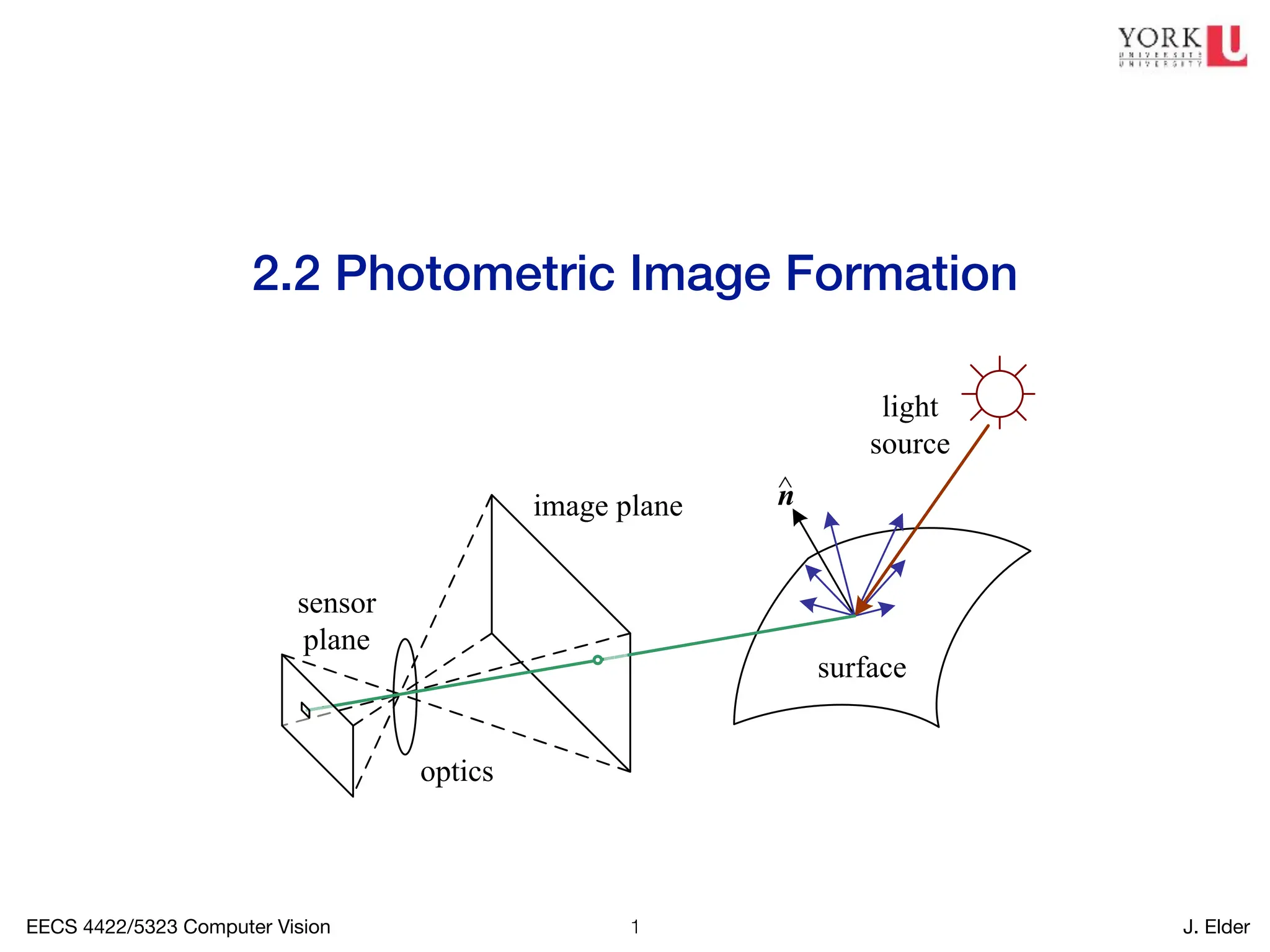
2.2 Photometric Image Formation
!1
2.2 Photometric image formation 61
n
^
surface
light
source
image plane
sensor
plane
optics
Figure 2.14 A simplified model of photometric image formation. Light is emitted by on
or more light sources and is then reflected from an object’s surface. A portion of this light i

Illumination
!2
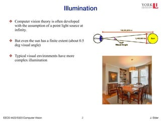
❖ Computer vision theory is often developed
with the assumption of a point light source at
infinity.
❖ But even the sun has a finite extent (about 0.5
deg visual angle)
❖ Typical visual environments have more
complex illumination

Measuring the Light Field
!3
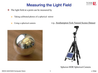
❖ The light field at a point can be measured by
๏ Taking calibrated photos of a spherical mirror
๏ Using a spherical camera
Spheron HDR Spherical Camera
e.g., Southampton-York Natural Scenes Dataset

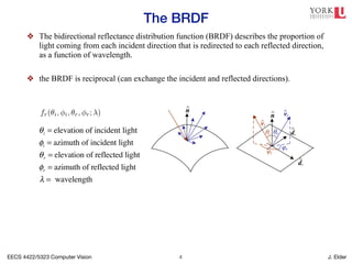
The BRDF
!4
❖ The bidirectional reflectance distribution function (BRDF) describes the proportion of
light coming from each incident direction that is redirected to each reflected direction,
as a function of wavelength.
❖ the BRDF is reciprocal (can exchange the incident and reflected directions).
els can be used to compute the global illumination corresponding to a
flectance Distribution Function (BRDF)
el of light scattering is the bidirectional reflectance distribution func-
e to some local coordinate frame on the surface, the BRDF is a four-
hat describes how much of each wavelength arriving at an incident
in a reflected direction v̂r (Figure 2.15b). The function can be written
of the incident and reflected directions relative to the surface frame as
fr(✓i, i, ✓r, r; ). (2.81)
al, i.e., because of the physics of light transport, you can interchange
and still get the same answer (this is sometimes called Helmholtz
neral models of light transport exist, including some that model spatial variation along
tering, and atmospheric effects—see Section 12.7.1—(Dorsey, Rushmeier, and Sillion
ensch et al. 2008).
θi = elevation of incident light
φi = azimuth of incident light
θr = elevation of reflected light
φr = azimuth of reflected light
λ = wavelength
62 Computer Vision: Algorithms and Applications (September 3, 2010 dra
n
^
vi
dx
n
^ vr
^
dy
^
θi
φi
φr
θr
^
^
(a) (b)
Figure 2.15 (a) Light scatters when it hits a surface. (b) The bidirectional reflectan
distribution function (BRDF) f(✓i, i, ✓r, r) is parameterized by the angles that the inc
dent, v̂i, and reflected, v̂r, light ray directions make with the local surface coordinate fram
( ˆ
dx, ˆ
dy, n̂).
2.2.2 Reflectance and shading
When light hits an object’s surface, it is scattered and reflected (Figure 2.15a). Many differe

The BRDF
!5
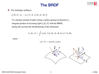
❖ For isotropic surfaces:
62 Computer Vision: Algorithms and Applications (September 3, 2010 d
n
^
vi
dx
n
^ vr
^
dy
^
θi
φi
φr
θr
^
^
(a) (b)
Figure 2.15 (a) Light scatters when it hits a surface. (b) The bidirectional reflect
distribution function (BRDF) f(✓i, i, ✓r, r) is parameterized by the angles that the
surfaces are isotropic, i.e., there are no preferred directions on the surface as far
ansport is concerned. (The exceptions are anisotropic surfaces such as brushed
) aluminum, where the reflectance depends on the light orientation relative to the
of the scratches.) For an isotropic material, we can simplify the BRDF to
fr(✓i, ✓r, | r i|; ) or fr(v̂i, v̂r, n̂; ), (2.82)
quantities ✓i, ✓r and r i can be computed from the directions v̂i, v̂r, and n̂.
culate the amount of light exiting a surface point p in a direction v̂r under a given
ondition, we integrate the product of the incoming light Li(v̂i; ) with the BRDF
hors call this step a convolution). Taking into account the foreshortening factor
we obtain
Lr(v̂r; ) =
Z
Li(v̂i; )fr(v̂i, v̂r, n̂; ) cos+
✓i dv̂i, (2.83)
cos+
✓i = max(0, cos ✓i). (2.84)
t sources are discrete (a finite number of point light sources), we can replace the
ith a summation,
Lr(v̂r; ) =
X
i
Li( )fr(v̂i, v̂r, n̂; ) cos+
✓i. (2.85)
s for a given surface can be obtained through physical modeling (Torrance and
967; Cook and Torrance 1982; Glassner 1995), heuristic modeling (Phong 1975), or
mpirical observation (Ward 1992; Westin, Arvo, and Torrance 1992; Dana, van Gin-
yar et al. 1999; Dorsey, Rushmeier, and Sillion 2007; Weyrich, Lawrence, Lensch
To calculate amount of light exiting a surface point p in direction v̂r ,
integrate product of incoming light Li v̂i;λ
( ) with the BRDF,
taking into account the foreshortening of the illuminant:
as light transport is concerned. (The exceptions are anisotropic surfaces such as brushed
(scratched) aluminum, where the reflectance depends on the light orientation relative to the
direction of the scratches.) For an isotropic material, we can simplify the BRDF to
fr(✓i, ✓r, | r i|; ) or fr(v̂i, v̂r, n̂; ), (2.82)
since the quantities ✓i, ✓r and r i can be computed from the directions v̂i, v̂r, and n̂.
To calculate the amount of light exiting a surface point p in a direction v̂r under a given
lighting condition, we integrate the product of the incoming light Li(v̂i; ) with the BRDF
(some authors call this step a convolution). Taking into account the foreshortening factor
cos+
✓i, we obtain
Lr(v̂r; ) =
Z
Li(v̂i; )fr(v̂i, v̂r, n̂; ) cos+
✓i dv̂i, (2.83)
where
cos+
✓i = max(0, cos ✓i). (2.84)
If the light sources are discrete (a finite number of point light sources), we can replace the
integral with a summation,
Lr(v̂r; ) =
X
i
Li( )fr(v̂i, v̂r, n̂; ) cos+
✓i. (2.85)
BRDFs for a given surface can be obtained through physical modeling (Torrance and
Sparrow 1967; Cook and Torrance 1982; Glassner 1995), heuristic modeling (Phong 1975), or
through empirical observation (Ward 1992; Westin, Arvo, and Torrance 1992; Dana, van Gin-
neken, Nayar et al. 1999; Dorsey, Rushmeier, and Sillion 2007; Weyrich, Lawrence, Lensch
et al. 2008).6
Typical BRDFs can often be split into their diffuse and specular components,

Diffuse (Lambertian, Matte) Reflection
!6
❖ The diffuse component of the BRDF scatters light
uniformly, giving rise to Lambertian shading.
❖ Colour of reflected light greatly influenced by material
❖ The amount of light reflected still depends upon the
incident elevation angle due to the foreshortening factor
flection, as well as darkening in the grooves and creases due to reduced
nterreflections. (Photo courtesy of the Caltech Vision Lab, http://www.
rchive.html.)
attered uniformly in all directions, i.e., the BRDF is constant,
fd(v̂i, v̂r, n̂; ) = fd( ), (2.86)
depends on the angle between the incident light direction and the surface
ecause the surface area exposed to a given amount of light becomes larger
coming completely self-shadowed as the outgoing surface normal points
(Figure 2.17a). (Think about how you orient yourself towards the sun or
imum warmth and how a flashlight projected obliquely against a wall is
pointing directly at it.) The shading equation for diffuse reflection can
) =
X
i
Li( )fd( ) cos+
✓i =
X
i
Li( )fd( )[v̂i · n̂]+
, (2.87)
[v̂i · n̂]+
= max(0, v̂i · n̂). (2.88)
omponent of a typical BRDF is specular (gloss or highlight) reflection,
ngly on the direction of the outgoing light. Consider light reflecting off a
gure 2.17b). Incident light rays are reflected in a direction that is rotated
COMP 557 12 - Lighting, Material, Shading
We now move to third part of the course where we will be concerned mostly with w
values to put at each pixel in an image. We will begin with a few simple models o
surface reflectance. I discussed these qualitatively, and then gave a more detailed
description of the model.
mirror
glossy
LIGHTING MATERIAL
parallel
ambient
point
spot
ambient
diffuse
(OpenGL
2.2 Photometric image formation
vi•n = 1
^ ^
0 < vi•n < 1
^ ^
vi•n < 0
^ ^
vi•n = 0
^ ^
(a)
While light is scattered uniformly in all directions, i.e., the BRDF is constant,
fd(v̂i, v̂r, n̂; ) = fd( ), (2.86)
he amount of light depends on the angle between the incident light direction and the surface
normal ✓i. This is because the surface area exposed to a given amount of light becomes larger
at oblique angles, becoming completely self-shadowed as the outgoing surface normal points
away from the light (Figure 2.17a). (Think about how you orient yourself towards the sun or
fireplace to get maximum warmth and how a flashlight projected obliquely against a wall is
ess bright than one pointing directly at it.) The shading equation for diffuse reflection can
hus be written as
Ld(v̂r; ) =
X
i
Li( )fd( ) cos+
✓i =
X
i
Li( )fd( )[v̂i · n̂]+
, (2.87)
where
[v̂i · n̂]+
= max(0, v̂i · n̂). (2.88)
Specular reflection
The second major component of a typical BRDF is specular (gloss or highlight) reflection,
which depends strongly on the direction of the outgoing light. Consider light reflecting off a
mirrored surface (Figure 2.17b). Incident light rays are reflected in a direction that is rotated
by 180 around the surface normal n̂. Using the same notation as in Equations (2.29–2.30),
archive.html.)
scattered uniformly in all directions, i.e., the BRDF is constant,
fd(v̂i, v̂r, n̂; ) = fd( ), (2.86)
t depends on the angle between the incident light direction and the surface
because the surface area exposed to a given amount of light becomes larger
becoming completely self-shadowed as the outgoing surface normal points
ht (Figure 2.17a). (Think about how you orient yourself towards the sun or
aximum warmth and how a flashlight projected obliquely against a wall is
ne pointing directly at it.) The shading equation for diffuse reflection can
r; ) =
X
i
Li( )fd( ) cos+
✓i =
X
i
Li( )fd( )[v̂i · n̂]+
, (2.87)
[v̂i · n̂]+
= max(0, v̂i · n̂). (2.88)
n
component of a typical BRDF is specular (gloss or highlight) reflection,
ongly on the direction of the outgoing light. Consider light reflecting off a
Figure 2.17b). Incident light rays are reflected in a direction that is rotated
e surface normal n̂. Using the same notation as in Equations (2.29–2.30),
where
Johann Heinrich Lambert (1728–1777)

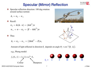
Specular (Mirror) Reflection
!7
❖ Specular reflection direction: 180 deg rotation
around surface normal.
vi•n = 1
^ ^
0 < vi•n < 1
^ ^
vi•n < 0
^ ^
vi•n = 0
^ ^
vi
v┴
n
^
v║ -v┴
si
180°
v║
^
^
(a) (b)
Figure 2.17 (a) The diminution of returned light caused by foreshortening depends on v̂i ·n̂,
the cosine of the angle between the incident light direction v̂i and the surface normal n̂. (b)
Mirror (specular) reflection: The incident light ray direction v̂i is reflected onto the specular
direction ŝi around the surface normal n̂.
we can compute the specular reflection direction ŝi as
ŝi = vk v? = (2n̂n̂T
I)vi. (2.89)
to be a set of uni-axial transforms, they can always be represented using
d transformations.
ntial twist)
presented by a rotation axis n̂ and an angle ✓, or equivalently by a 3D
gure 2.5 shows how we can compute the equivalent rotation. First, we
onto the axis n̂ to obtain
vk = n̂(n̂ · v) = (n̂n̂T
)v, (2.29)
nent of v that is not affected by the rotation. Next, we compute the
al of v from n̂,
v? = v vk = (I n̂n̂T
)v. (2.30)
metimes referred to as gimbal lock.
epresented by a rotation axis n̂ and an angle ✓, or equivalently by a 3D
igure 2.5 shows how we can compute the equivalent rotation. First, we
onto the axis n̂ to obtain
vk = n̂(n̂ · v) = (n̂n̂T
)v, (2.29)
onent of v that is not affected by the rotation. Next, we compute the
ual of v from n̂,
v? = v vk = (I n̂n̂T
)v. (2.30)
sometimes referred to as gimbal lock.
vi•n < 0
^ ^
v┴
v║ -v┴
180°
(a) (b)
The diminution of returned light caused by foreshortening depends on v̂i ·n̂,
angle between the incident light direction v̂i and the surface normal n̂. (b)
reflection: The incident light ray direction v̂i is reflected onto the specular
nd the surface normal n̂.
he specular reflection direction ŝi as
ŝi = vk v? = (2n̂n̂T
I)vi. (2.89)
of light reflected in a given direction v̂r thus depends on the angle ✓s =
tween the view direction v̂r and the specular direction ŝi. For example, the
del uses a power of the cosine of the angle,
fs(✓s; ) = ks( ) coske
✓s, (2.90)
reflection: The incident light ray direction v̂i is reflected onto the specular
nd the surface normal n̂.
he specular reflection direction ŝi as
ŝi = vk v? = (2n̂n̂T
I)vi. (2.89)
of light reflected in a given direction v̂r thus depends on the angle ✓s =
tween the view direction v̂r and the specular direction ŝi. For example, the
del uses a power of the cosine of the angle,
✓s, (2.90)
e and Sparrow (1967) micro-facet model uses a Gaussian,
fs(✓s; ) = ks( ) exp( c2
s✓2
s). (2.91)
ke (or inverse Gaussian widths cs) correspond to more specular surfaces
lights, while smaller exponents better model materials with softer gloss.
❖ Recall:
❖ Thus
Amount of light reflected in direction v̂r depends on angle θs = cos−1
v̂r ⋅ŝi
( ).
e.g., Phong model:
vi•n < 0
^ ^
v┴
v║ -v┴
180°
(a) (b)
he diminution of returned light caused by foreshortening depends on v̂i ·n̂,
ngle between the incident light direction v̂i and the surface normal n̂. (b)
eflection: The incident light ray direction v̂i is reflected onto the specular
the surface normal n̂.
e specular reflection direction ŝi as
ŝi = vk v? = (2n̂n̂T
I)vi. (2.89)
light reflected in a given direction v̂r thus depends on the angle ✓s =
ween the view direction v̂r and the specular direction ŝi. For example, the
el uses a power of the cosine of the angle,
✓s, (2.90)
and Sparrow (1967) micro-facet model uses a Gaussian,
f (✓ ; ) = k ( ) exp( c2
✓2
). (2.91)
ke =
Colour Sharpness

Phong Shading
!8
❖ The full Phong model combines diffuse and specular components contributed by the
main illuminant with an ambient term that attempts to account for all other light
incident upon the surface from other parts of the scene (sky, walls, etc.)
Bui Tuong Phong (1942-1975)
blue sky. In the Phong model, the ambient term does not depend on surface orientation, but
depends on the color of both the ambient illumination La( ) and the object ka( ),
fa( ) = ka( )La( ). (2.92)
Putting all of these terms together, we arrive at the Phong shading model,
Lr(v̂r; ) = ka( )La( ) + kd( )
X
i
Li( )[v̂i · n̂]+
+ ks( )
X
i
Li( )(v̂r · ŝi)ke
. (2.93)
Figure 2.18 shows a typical set of Phong shading model components as a function of the
angle away from the surface normal (in a plane containing both the lighting direction and the
viewer).
Typically, the ambient and diffuse reflection color distributions ka( ) and kd( ) are the
same, since they are both due to sub-surface scattering (body reflection) inside the surface
material (Shafer 1985). The specular reflection distribution ks( ) is often uniform (white),
since it is caused by interface reflections that do not change the light color. (The exception
to this are metallic materials, such as copper, as opposed to the more common dielectric
materials, such as plastics.)
The ambient illumination La( ) often has a different color cast from the direct light
sources Li( ), e.g., it may be blue for a sunny outdoor scene or yellow for an interior lit
with candles or incandescent lights. (The presence of ambient sky illumination in shadowed
areas is what often causes shadows to appear bluer than the corresponding lit portions of a
scene). Note also that the diffuse component of the Phong model (or of any shading model)
depends on the angle of the incoming light source v̂ , while the specular component depends
Ambient Diffuse Specular
NB: I can’t make sense of Fig. 2.18: please ignore.
ka λ
( ) ! kd λ
( ) (both due to sub-surface scatter).
ks λ
( ) ! constant, thus specularity assumes colour of illuminant.
❖ Typically:
La λ
( )≠ Li λ
( )

Ray Tracing
!9
❖ The Phong model assumes a finite number of discrete light sources.
❖ Light emitted by these sources bounces off the surface and into the camera.
❖ In reality, some of these sources may be shadowed by other objects, and the surface is
generally also illuminated by inter-reflections (multiple bounces)
❖ Two approaches, depending on nature of scene:
๏ If mostly specular, use ray tracing:
✦ Follow each ray from camera across multiple bounces toward light sources
๏ If mostly matte, use radiosity:
✦ Model light interchanged between all pairs of surface patches, and then solve as linear system
with light sources as forcing function.
5
Relationship between shadows and interreflections. Though historically ignored,
the interaction of light with objects results in a number of subtle illumination effects
which may be useful cues for surface attributes and relations. As noted above, cast
shadows are effective in determining the 3D layout of a scene, and other studies are
finding shadows play a role in object recognition [1,2,6] Interreflection is another effect
that is closely related to shadows [7]. Consider the intersection of two surfaces (figure
3).

Optics
!10
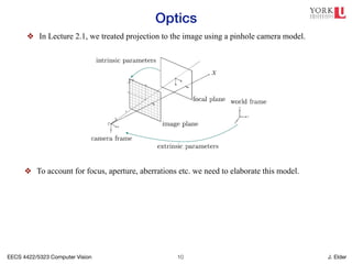
❖ In Lecture 2.1, we treated projection to the image using a pinhole camera model.
❖ To account for focus, aperture, aberrations etc. we need to elaborate this model.

Thin Lens Model
!11
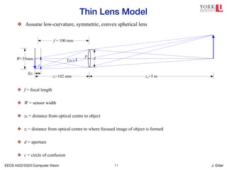
❖ f = focal length
❖ W = sensor width
❖ z0 = distance from optical centre to object
❖ zi = distance from optical centre to where focused image of object is formed
❖ d = aperture
❖ c = circle of confusion
zi=102 mm
f = 100 mm
W=35mm
zo=5 m
f.o.v.
c
Δzi
P d
Figure 2.19 A thin lens of focal length f focuses the light from a plane a distance zo in front
of the lens at a distance zi behind the lens, where 1
zo
+ 1
zi
= 1
f . If the focal plane (vertical
gray line next to c) is moved forward, the images are no longer in focus and the circle of
confusion c (small thick line segments) depends on the distance of the image plane motion
zi relative to the lens aperture diameter d. The field of view (f.o.v.) depends on the ratio
between the sensor width W and the focal length f (or, more precisely, the focusing distance
zi, which is usually quite close to f).
ration, we need to develop a more sophisticated model, which is where the study of optics
comes in (Möller 1988; Hecht 2001; Ray 2002).
❖ Assume low-curvature, symmetric, convex spherical lens

Lens Equation
!12
❖ If the sensor plane does not lie at zi, a point on the object
will be imaged as a blurred disk ( the circle of confusion c).
❖ Allowable depth variation that limits this blur to an
acceptable level called the depth of field.
❖ Depth of field increases with larger apertures and longer
viewing distances.
zi=102 mm
f = 100 mm
W=35mm
zo=5 m
f.o.v.
c
Δzi
P d
Figure 2.19 A thin lens of focal length f focuses the light from a plane a distance zo in front
of the lens at a distance zi behind the lens, where 1
zo
+ 1
zi
= 1
f . If the focal plane (vertical
gray line next to c) is moved forward, the images are no longer in focus and the circle of
confusion c (small thick line segments) depends on the distance of the image plane motion
zi relative to the lens aperture diameter d. The field of view (f.o.v.) depends on the ratio
between the sensor width W and the focal length f (or, more precisely, the focusing distance
zi, which is usually quite close to f).
ration, we need to develop a more sophisticated model, which is where the study of optics
comes in (Möller 1988; Hecht 2001; Ray 2002).
Figure 2.19 shows a diagram of the most basic lens model, i.e., the thin lens composed
of a single piece of glass with very low, equal curvature on both sides. According to the
ose to f).
a more sophisticated model, which is where the study of optics
cht 2001; Ray 2002).
agram of the most basic lens model, i.e., the thin lens composed
with very low, equal curvature on both sides. According to the
ved using simple geometric arguments on light ray refraction), the
stance to an object zo and the distance behind the lens at which a
can be expressed as
1
zo
+
1
zi
=
1
f
, (2.96)
ength of the lens. If we let zo ! 1, i.e., we adjust the lens (move
ects at infinity are in focus, we get zi = f, which is why we can
th f as being equivalent (to a first approximation) to a pinhole a
ane (Figure 2.10), whose field of view is given by (2.60).
ved away from its proper in-focus setting of zi (e.g., by twisting
objects at zo are no longer in focus, as shown by the gray plane in
mis-focus is measured by the circle of confusion c (shown as short
the gray plane).7
The equation for the circle of confusion can be
gles; it depends on the distance of travel in the focal plane zi
distance zi and the diameter of the aperture d (see Exercise 2.4).
Note that lim
z0→∞
zi = f .
70 Computer Vision: Algorithms and Application
(a)
Figure 2.20 Regular and zoom lens depth of field
The allowable depth variation in the scene that limits the circle
able number is commonly called the depth of field and is a functio
and the aperture, as shown diagrammatically by many lens markin
depth of field depends on the aperture diameter d, we also have to
the commonly displayed f-number, which is usually denoted as f
f/# = N =
f
d
,
where the focal length f and the aperture diameter d are measu
millimeters).
The usual way to write the f-number is to replace the # in f/
f-number (f-stop) = f / d.

Chromatic Aberration
!13
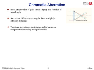
❖ Index of refraction of glass varies slightly as a function of
wavelength.
❖ As a result, different wavelengths focus at slightly
different distances.
❖ To reduce aberrations, most photographic lenses are
compound lenses using multiple elements.

Computer_vision-photometric_image_formation.pdf

More Related Content

Similar to Computer_vision-photometric_image_formation.pdf

Recently uploaded

Computer_vision-photometric_image_formation.pdf