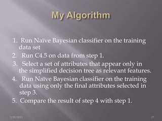
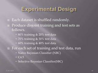
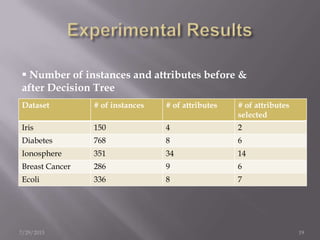
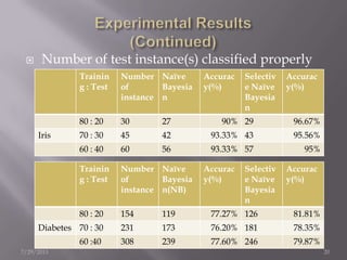
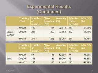
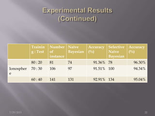
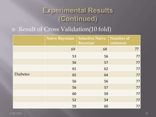
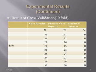
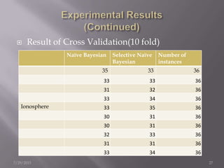
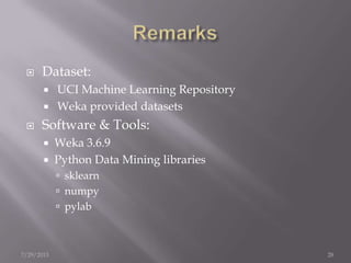
2. Abstract of the work
Why we need it?
Naïve Bayesian Classifier
Definition
Algorithm
Gaussian Distribution
Decision Tree
Definition
Algorithm
7/29/2013 2
3. Information Gain
My Algorithm
Experimental Design
Experimental Result
Remarks
7/29/2013 3
4. Apply Naïve Bayesian.
Based on information gain create decision tree
& select attributes.
Apply Naïve Bayesian with the selected
attributes.
Minimize the time & space need to analysis.
Can work with continuous data stream.
7/29/2013 4
5. 1. Now-a-days data volume of internet
user is getting larger.
2. Machine learning is getting harder
day by day.
3. Pre-processing of data may be a
solution for it.
4. Using the necessary data only can
make the learning process faster
7/29/2013 5
6. 5. A better technique can make the process more
organized using only necessary data
6. Cut off all un-important attributes from data set.
7. Dataset become compact in terms of attributes
and calculation becomes fast.
8. Get better performance than past on behalf of
time and space.
7/29/2013 6
7. Naïve Bayesian Classifier
Gaussian Distribution
Decision Tree
Information Gain
7/29/2013 7
8. The Naïve Bayesian classifier(NB) is a
straightforward and frequently used method
for supervised learning.
It provides a flexible way for dealing with any
number of attributes or classes
It’s based on statistical probability theory.
7/29/2013 8
9. It is the asymptotically fastest learning
algorithm that examines all its training input.
It has been demonstrated to perform
surprisingly well in a very wide variety of
problems in spite of the simplistic nature of the
model.
Furthermore, small amounts of bad data, or
“noise,” do not perturb the results by much.
7/29/2013 9
10. There are classes, say Ck for the data to be
classified into.
Each class has a probability P(Ck) that
represents the prior probability of classifying
an attribute into Ck.
For n attribute values, vj, the goal of
classification is clearly to find the conditional
probability P(Ck | v1 ∧ v2 ∧ … ∧ vn).
7/29/2013 10
11. By Bayes’ rule, this probability is equivalent to
7/29/2013 11
12. The mathematical function for calculating the
probability density of Gaussian distribution at a
particular point X is:
where µ is the mean and σ is the standard deviation of
the continues-valued attribute X
7/29/2013 12
13. 1. Decision trees are one of the most
popular methods used for inductive
inference.
2. The basic algorithm for decision tree
induction is a greedy algorithm that
constructs decision trees in a top-down
recursive divide-and-conquer manner.
3. The main concept of selecting an
attribute and constructing a decision tree
is Information Gain(IG)
7/29/2013 13
14. The basic idea behind any decision tree
algorithm is as follows:
Choose the best attribute(s) to split the remaining
instances and make that attribute a decision node
using Information Gain
Repeat this process for recursively for each child
Stop when:
All the instances have the same target attribute value
There are no more attributes
There are no more instances
7/29/2013 14
15. Leave At
Stall? Accident?
10 AM 9 AM
8 AM
Long
Long
Short Medium Long
No Yes No Yes
If we leave at
9 AM and
there is no
accident
happened on
the road, what
will our
commute time
be?
16. The critical step in decision trees is the selection of
the best test attribute.
The information gain measure is used to select the
test attribute at each node in the tree.
The expected information needed to classify a
given sample is given by
where pk is the probability that an arbitrary sample
belongs to class Ck and is estimated by sk / s.
7/29/2013 16
17. 1. Run Naïve Bayesian classifier on the training
data set
2. Run C4.5 on data from step 1.
3. Select a set of attributes that appear only in
the simplified decision tree as relevant features.
4. Run Naïve Bayesian classifier on the training
data using only the final attributes selected in
step 3.
5. Compare the result of step 4 with step 1.
7/29/2013 17
18. Each dataset is shuffled randomly.
Produce disjoint training and test sets as
follows.
80% training & 20% test data
70% training & 30% test data
60% training & 40% test data
For each set of training and test data, run
Naïve Bayesian Classifier (NBC)
C4.5
Selective Bayesian Classifier(SBC)
7/29/2013 18
19. Dataset # of instances # of attributes # of attributes
selected
Iris 150 4 2
Diabetes 768 8 6
Ionosphere 351 34 14
Breast Cancer 286 9 6
Ecoli 336 8 7
7/29/2013 19
Number of instances and attributes before &
after Decision Tree
20. Number of test instance(s) classified properly
7/29/2013 20
Trainin
g : Test
Number
of
instance
Naïve
Bayesia
n
Accurac
y(%)
Selectiv
e Naïve
Bayesia
n
Accurac
y(%)
80 : 20 30 27 90% 29 96.67%
Iris 70 : 30 45 42 93.33% 43 95.56%
60 : 40 60 56 93.33% 57 95%
Trainin
g : Test
Number
of
instance
Naïve
Bayesia
n(NB)
Accurac
y(%)
Selectiv
e Naïve
Bayesia
n
Accurac
y(%)
80 : 20 154 119 77.27% 126 81.81%
Diabetes 70 : 30 231 173 76.20% 181 78.35%
60 :40 308 239 77.60% 246 79.87%