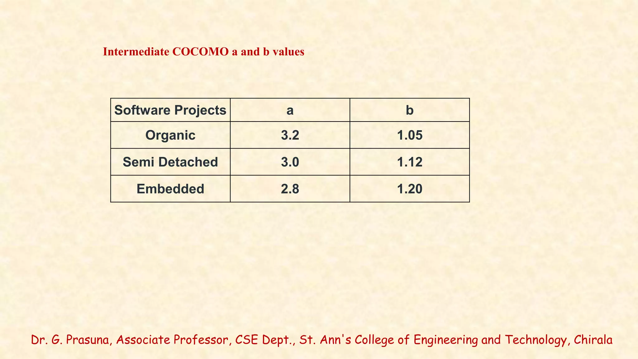
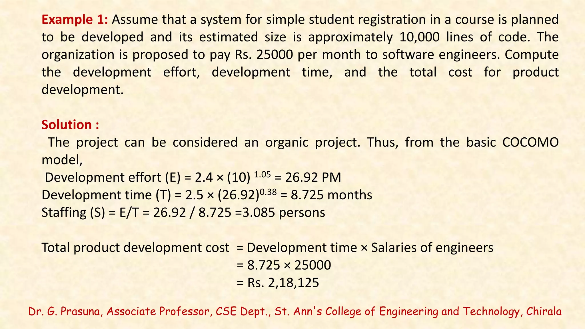
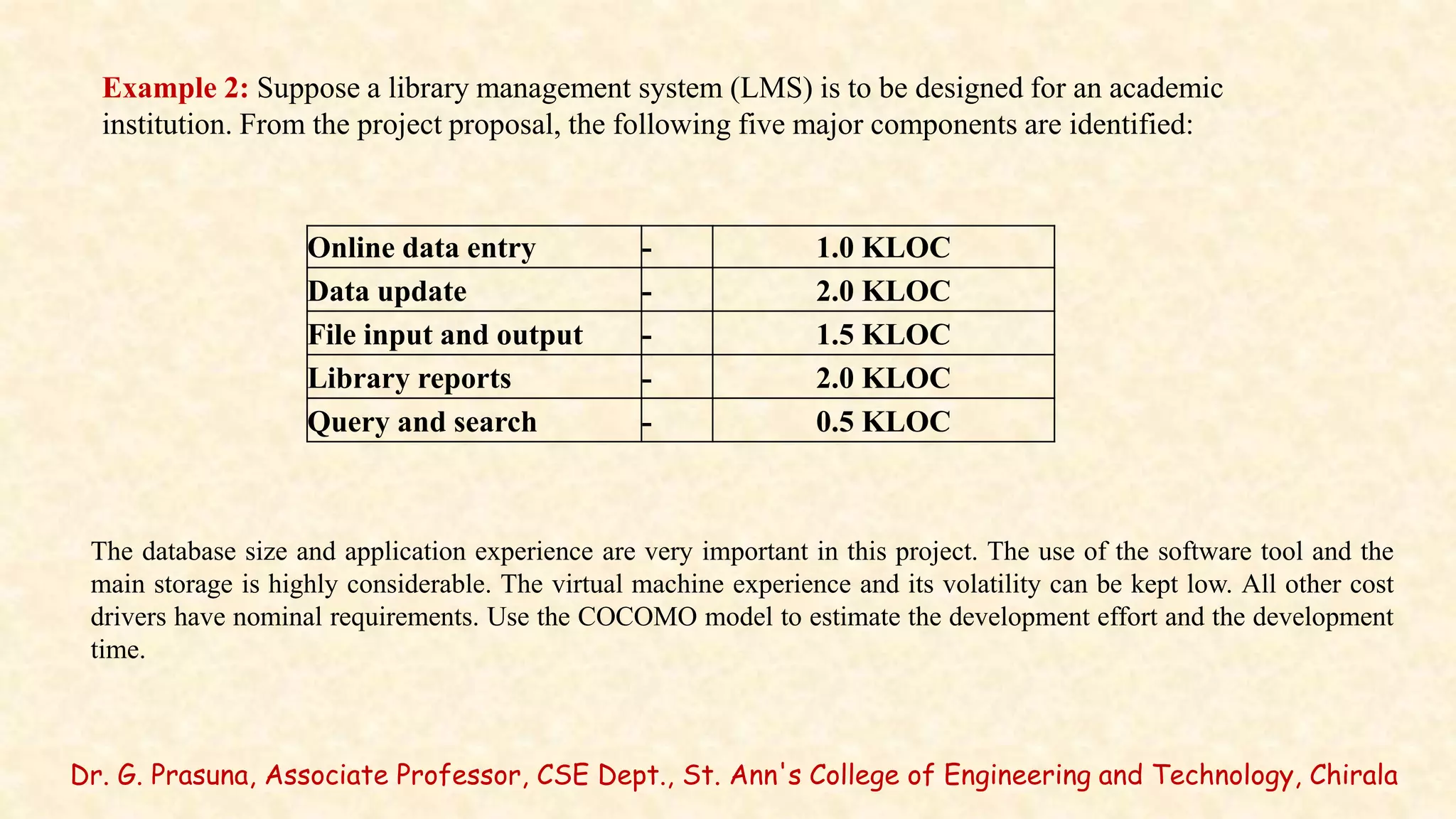
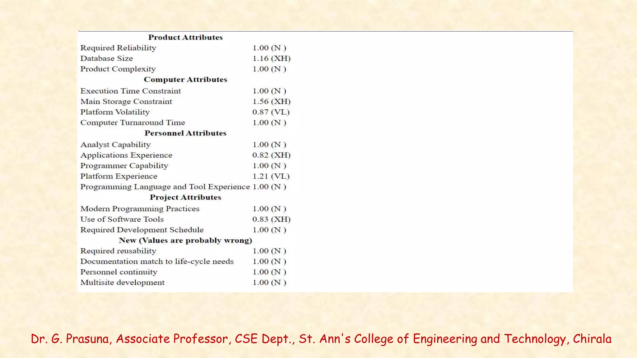
Dr. G. Prasuna, Associate Professor, CSE Dept., St. Ann's College of Engineering and Technology, Chirala
SOFTWARE ENGINEERING LAB
JNTUK R20
Exercise 5: COCOMO Model
Ex-5 Consider any application, using COCOMO
model, estimate the effort.
Dr. G. Prasuna, Associate Professor, CSE Dept., St. Ann's College of Engineering and Technology, Chirala
Exercise 5: Consider any application, using COCOMO model,
estimate the effort.
AIM: Estimating Effort using COCOMO model
Dr. G. Prasuna, Associate Professor, CSE Dept., St. Ann's College of Engineering and Technology, Chirala
COCOMO Model
COCOMO (COnstructive COst MOdel) is an algorithmic cost estimation technique proposed
by Boehm, which works in a bottom-up manner.
It is designed to provide some mathematical equations to estimate software projects.
These mathematical equations are based on historical data and use project size in the form of
KLOC.
The COCOMO model uses a multivariable size estimation model for effort estimation.
A multivariable model depends on several variables, such as development environment, user
involvement, memory constraints, technique used, etc.
COCOMO estimation is a family of hierarchical models, which includes
•Basic,
•Intermediate, and
•Detailed COCOMO models.
Each of the models initially estimates efforts based on the total estimated KLOC.
Dr. G. Prasuna, Associate Professor, CSE Dept., St. Ann's College of Engineering and Technology, Chirala
Basic COCOMO Model
The basic COCOMO model estimates effort in a function of the estimated KLOC in the
proposed project.
The basic COCOMO model is very simple, quick, and applicable to small to medium organic-
type projects. It is given as follows:
Development effort (E) = a × (KLOC) b Development time (T) = c × (E) d
Where a, b, c, and d are constants and these values are determined from the historical data
of the past projects.
The development time (T) is calculated from the initial development effort (E).
Dr. G. Prasuna, Associate Professor, CSE Dept., St. Ann's College of Engineering and Technology, Chirala
Boehm’s definition of Organic, Semid-detached, and Embedded systems are
elaborated below:
Organic: A development project can be considered as organic type, if the
project deals with developing a well understood application program.
Semidetached: A development project can be considered as Semidetached type,
if the
development consists of a mixture of experience and inexperience in developing
the project.
Embedded: A development project can be considered as embedded-type, if the
software being developed is strongly coupled to complex hardware.
Dr. G. Prasuna, Associate Professor, CSE Dept., St. Ann's College of Engineering and Technology, Chirala
The values of a, b, c and d for organic, semidetached, and embedded-type
projects are shown in Table.
Software Projects a b c d
Organic 2.4 1.05 2.5 0.38
Semi Detached 3.0 1.12 2.5 0.35
Embedded 3.6 1.20 2.5 0.32
Dr. G. Prasuna, Associate Professor, CSE Dept., St. Ann's College of Engineering and Technology, Chirala
Intermediate COCOMO Model
Boehm has introduced 15 cost drivers, considering the various aspects of product development
environment. These cost drivers are used to adjust the project complexity for estimation of effort and these are
termed as effort adjustment factors (EAF).
These cost drivers are classified as computer attributes, product attributes, project attributes, and
personnel attributes.
The intermediate COCOMO model computes software development effort as a function of the program size
and a set of cost drivers.
The intermediate COCOMO model estimates the initial effort using the basic COCOMO model. Then the
EAF is calculated as the product of 15 cost drivers.
Total effort is determined by multiplying the initial effort with the total value of EAF. The computation steps
are summarized below.
Development effort (E):
Initial effort (Ei) = a × (KLOC) b
EAF= EAF1 × EAF 2 ×... × EAF n
Total development effort (E)= Ei× EAF
Development time (T) = c * (E)d
Dr. G. Prasuna, Associate Professor, CSE Dept., St. Ann's College of Engineering and Technology, Chirala
(iii) Personnel attributes –
• Analyst capability
• Software engineering capability
• Applications experience
• Virtual machine experience
• Programming language experience
(iv) Project attributes –
• Use of software tools
• Application of software engineering methods
• Required development schedule
Intermediate Model utilizes 15 such drivers for cost estimation. Classification of Cost
Drivers and their attributes:
Dr. G. Prasuna, Associate Professor, CSE Dept., St. Ann's College of Engineering and Technology, Chirala
Cost Drivers Very Low Low Nominal High Very High
Product Attributes
Required Software Reliability 0.75 0.88 1.00 1.15 1.40
Size of Application Database 0.94 1.00 1.08 1.16
Complexity of The Product 0.70 0.85 1.00 1.15 1.30
Hardware Attributes
Runtime Performance Constraints 1.00 1.11 1.30
Memory Constraints 1.00 1.06 1.21
Volatility of the virtual machine environment 0.87 1.00 1.15 1.30
Required turnabout time 0.94 1.00 1.07 1.15
Personnel attributes
Analyst capability 1.46 1.19 1.00 0.86 0.71
Applications experience 1.29 1.13 1.00 0.91 0.82
Software engineer capability 1.42 1.17 1.00 0.86 0.70
Virtual machine experience 1.21 1.10 1.00 0.90
Programming language experience 1.14 1.07 1.00 0.95
Project Attributes
Application of software engineering methods 1.24 1.10 1.00 0.91 0.82
Use of software tools 1.24 1.10 1.00 0.91 0.83
Required development schedule 1.23 1.08 1.00 1.04 1.10
Dr. G. Prasuna, Associate Professor, CSE Dept., St. Ann's College of Engineering and Technology, Chirala
Software Projects a b
Organic 3.2 1.05
Semi Detached 3.0 1.12
Embedded 2.8 1.20
Intermediate COCOMO a and b values
Dr. G. Prasuna, Associate Professor, CSE Dept., St. Ann's College of Engineering and Technology, Chirala
Example 1: Assume that a system for simple student registration in a course is planned
to be developed and its estimated size is approximately 10,000 lines of code. The
organization is proposed to pay Rs. 25000 per month to software engineers. Compute
the development effort, development time, and the total cost for product
development.
Solution :
The project can be considered an organic project. Thus, from the basic COCOMO
model,
Development effort (E) = 2.4 × (10) 1.05 = 26.92 PM
Development time (T) = 2.5 × (26.92)0.38 = 8.725 months
Staffing (S) = E/T = 26.92 / 8.725 =3.085 persons
Total product development cost = Development time × Salaries of engineers
= 8.725 × 25000
= Rs. 2,18,125
Dr. G. Prasuna, Associate Professor, CSE Dept., St. Ann's College of Engineering and Technology, Chirala
OUTPUT:
Dr. G. Prasuna, Associate Professor, CSE Dept., St. Ann's College of Engineering and Technology, Chirala
Example 2: Suppose a library management system (LMS) is to be designed for an academic
institution. From the project proposal, the following five major components are identified:
Online data entry - 1.0 KLOC
Data update - 2.0 KLOC
File input and output - 1.5 KLOC
Library reports - 2.0 KLOC
Query and search - 0.5 KLOC
The database size and application experience are very important in this project. The use of the software tool and the
main storage is highly considerable. The virtual machine experience and its volatility can be kept low. All other cost
drivers have nominal requirements. Use the COCOMO model to estimate the development effort and the development
time.
Dr. G. Prasuna, Associate Professor, CSE Dept., St. Ann's College of Engineering and Technology, Chirala
Solution: The LMS project can be considered an organic category project. The total
size of the modules is 7 KLOC. The development effort and development time can
be calculated as follows:
Development effort
Initial effort (Ei) = 3.2 × (7) 1.05=3.2*7.71=24.672 PM
EAF = 1.16*0.82*0.83*1.21*1.21*0.87 =1.0056
Total Effort (E) = 24.672*1.0056 =24.81 PM
Development time (T) = 2.5 × (E)0.38 month =2.5 *(24.81) 0.38 month
=2.5 *3.388 =8.47 months
Staffing (S) = E/T = 24.81 / 8.47 = 2.929 persons.
Dr. G. Prasuna, Associate Professor, CSE Dept., St. Ann's College of Engineering and Technology, Chirala
THANK YOU

COCOMO Model For Effort Estimation

  • 1.
    Dr. G. Prasuna,Associate Professor, CSE Dept., St. Ann's College of Engineering and Technology, Chirala SOFTWARE ENGINEERING LAB JNTUK R20 Exercise 5: COCOMO Model Ex-5 Consider any application, using COCOMO model, estimate the effort.
  • 2.
    Dr. G. Prasuna,Associate Professor, CSE Dept., St. Ann's College of Engineering and Technology, Chirala Exercise 5: Consider any application, using COCOMO model, estimate the effort. AIM: Estimating Effort using COCOMO model
  • 3.
    Dr. G. Prasuna,Associate Professor, CSE Dept., St. Ann's College of Engineering and Technology, Chirala COCOMO Model COCOMO (COnstructive COst MOdel) is an algorithmic cost estimation technique proposed by Boehm, which works in a bottom-up manner. It is designed to provide some mathematical equations to estimate software projects. These mathematical equations are based on historical data and use project size in the form of KLOC. The COCOMO model uses a multivariable size estimation model for effort estimation. A multivariable model depends on several variables, such as development environment, user involvement, memory constraints, technique used, etc. COCOMO estimation is a family of hierarchical models, which includes •Basic, •Intermediate, and •Detailed COCOMO models. Each of the models initially estimates efforts based on the total estimated KLOC.
  • 4.
    Dr. G. Prasuna,Associate Professor, CSE Dept., St. Ann's College of Engineering and Technology, Chirala Basic COCOMO Model The basic COCOMO model estimates effort in a function of the estimated KLOC in the proposed project. The basic COCOMO model is very simple, quick, and applicable to small to medium organic- type projects. It is given as follows: Development effort (E) = a × (KLOC) b Development time (T) = c × (E) d Where a, b, c, and d are constants and these values are determined from the historical data of the past projects. The development time (T) is calculated from the initial development effort (E).
  • 5.
    Dr. G. Prasuna,Associate Professor, CSE Dept., St. Ann's College of Engineering and Technology, Chirala Boehm’s definition of Organic, Semid-detached, and Embedded systems are elaborated below: Organic: A development project can be considered as organic type, if the project deals with developing a well understood application program. Semidetached: A development project can be considered as Semidetached type, if the development consists of a mixture of experience and inexperience in developing the project. Embedded: A development project can be considered as embedded-type, if the software being developed is strongly coupled to complex hardware.
  • 6.
    Dr. G. Prasuna,Associate Professor, CSE Dept., St. Ann's College of Engineering and Technology, Chirala The values of a, b, c and d for organic, semidetached, and embedded-type projects are shown in Table. Software Projects a b c d Organic 2.4 1.05 2.5 0.38 Semi Detached 3.0 1.12 2.5 0.35 Embedded 3.6 1.20 2.5 0.32
  • 7.
    Dr. G. Prasuna,Associate Professor, CSE Dept., St. Ann's College of Engineering and Technology, Chirala Intermediate COCOMO Model Boehm has introduced 15 cost drivers, considering the various aspects of product development environment. These cost drivers are used to adjust the project complexity for estimation of effort and these are termed as effort adjustment factors (EAF). These cost drivers are classified as computer attributes, product attributes, project attributes, and personnel attributes. The intermediate COCOMO model computes software development effort as a function of the program size and a set of cost drivers. The intermediate COCOMO model estimates the initial effort using the basic COCOMO model. Then the EAF is calculated as the product of 15 cost drivers. Total effort is determined by multiplying the initial effort with the total value of EAF. The computation steps are summarized below. Development effort (E): Initial effort (Ei) = a × (KLOC) b EAF= EAF1 × EAF 2 ×... × EAF n Total development effort (E)= Ei× EAF Development time (T) = c * (E)d
  • 8.
    Dr. G. Prasuna,Associate Professor, CSE Dept., St. Ann's College of Engineering and Technology, Chirala (iii) Personnel attributes – • Analyst capability • Software engineering capability • Applications experience • Virtual machine experience • Programming language experience (iv) Project attributes – • Use of software tools • Application of software engineering methods • Required development schedule Intermediate Model utilizes 15 such drivers for cost estimation. Classification of Cost Drivers and their attributes:
  • 9.
    Dr. G. Prasuna,Associate Professor, CSE Dept., St. Ann's College of Engineering and Technology, Chirala Cost Drivers Very Low Low Nominal High Very High Product Attributes Required Software Reliability 0.75 0.88 1.00 1.15 1.40 Size of Application Database 0.94 1.00 1.08 1.16 Complexity of The Product 0.70 0.85 1.00 1.15 1.30 Hardware Attributes Runtime Performance Constraints 1.00 1.11 1.30 Memory Constraints 1.00 1.06 1.21 Volatility of the virtual machine environment 0.87 1.00 1.15 1.30 Required turnabout time 0.94 1.00 1.07 1.15 Personnel attributes Analyst capability 1.46 1.19 1.00 0.86 0.71 Applications experience 1.29 1.13 1.00 0.91 0.82 Software engineer capability 1.42 1.17 1.00 0.86 0.70 Virtual machine experience 1.21 1.10 1.00 0.90 Programming language experience 1.14 1.07 1.00 0.95 Project Attributes Application of software engineering methods 1.24 1.10 1.00 0.91 0.82 Use of software tools 1.24 1.10 1.00 0.91 0.83 Required development schedule 1.23 1.08 1.00 1.04 1.10
  • 10.
    Dr. G. Prasuna,Associate Professor, CSE Dept., St. Ann's College of Engineering and Technology, Chirala Software Projects a b Organic 3.2 1.05 Semi Detached 3.0 1.12 Embedded 2.8 1.20 Intermediate COCOMO a and b values
  • 11.
    Dr. G. Prasuna,Associate Professor, CSE Dept., St. Ann's College of Engineering and Technology, Chirala Example 1: Assume that a system for simple student registration in a course is planned to be developed and its estimated size is approximately 10,000 lines of code. The organization is proposed to pay Rs. 25000 per month to software engineers. Compute the development effort, development time, and the total cost for product development. Solution : The project can be considered an organic project. Thus, from the basic COCOMO model, Development effort (E) = 2.4 × (10) 1.05 = 26.92 PM Development time (T) = 2.5 × (26.92)0.38 = 8.725 months Staffing (S) = E/T = 26.92 / 8.725 =3.085 persons Total product development cost = Development time × Salaries of engineers = 8.725 × 25000 = Rs. 2,18,125
  • 12.
    Dr. G. Prasuna,Associate Professor, CSE Dept., St. Ann's College of Engineering and Technology, Chirala OUTPUT:
  • 13.
    Dr. G. Prasuna,Associate Professor, CSE Dept., St. Ann's College of Engineering and Technology, Chirala Example 2: Suppose a library management system (LMS) is to be designed for an academic institution. From the project proposal, the following five major components are identified: Online data entry - 1.0 KLOC Data update - 2.0 KLOC File input and output - 1.5 KLOC Library reports - 2.0 KLOC Query and search - 0.5 KLOC The database size and application experience are very important in this project. The use of the software tool and the main storage is highly considerable. The virtual machine experience and its volatility can be kept low. All other cost drivers have nominal requirements. Use the COCOMO model to estimate the development effort and the development time.
  • 14.
    Dr. G. Prasuna,Associate Professor, CSE Dept., St. Ann's College of Engineering and Technology, Chirala Solution: The LMS project can be considered an organic category project. The total size of the modules is 7 KLOC. The development effort and development time can be calculated as follows: Development effort Initial effort (Ei) = 3.2 × (7) 1.05=3.2*7.71=24.672 PM EAF = 1.16*0.82*0.83*1.21*1.21*0.87 =1.0056 Total Effort (E) = 24.672*1.0056 =24.81 PM Development time (T) = 2.5 × (E)0.38 month =2.5 *(24.81) 0.38 month =2.5 *3.388 =8.47 months Staffing (S) = E/T = 24.81 / 8.47 = 2.929 persons.
  • 15.
    Dr. G. Prasuna,Associate Professor, CSE Dept., St. Ann's College of Engineering and Technology, Chirala
  • 16.
    Dr. G. Prasuna,Associate Professor, CSE Dept., St. Ann's College of Engineering and Technology, Chirala
  • 17.
    Dr. G. Prasuna,Associate Professor, CSE Dept., St. Ann's College of Engineering and Technology, Chirala
  • 18.
    Dr. G. Prasuna,Associate Professor, CSE Dept., St. Ann's College of Engineering and Technology, Chirala
  • 19.
    Dr. G. Prasuna,Associate Professor, CSE Dept., St. Ann's College of Engineering and Technology, Chirala THANK YOU