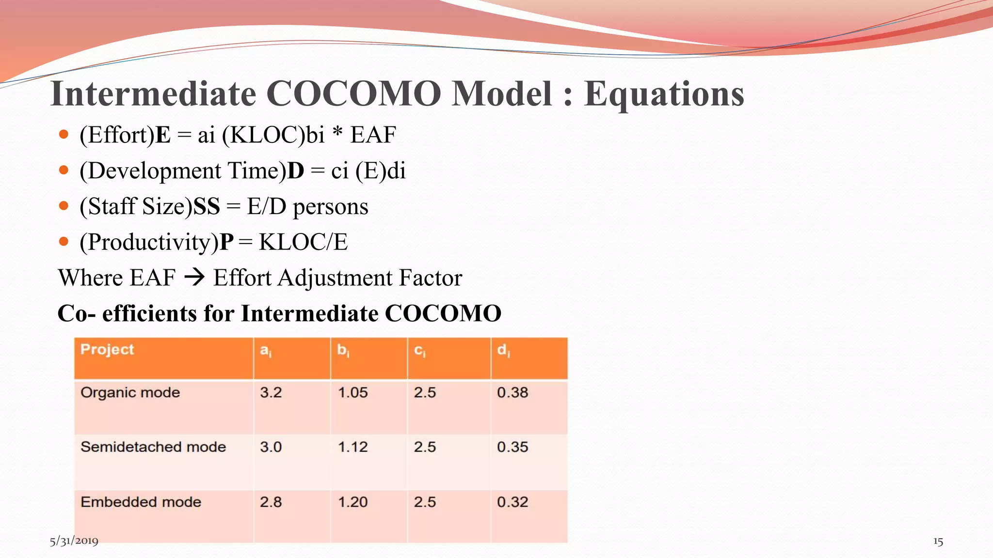
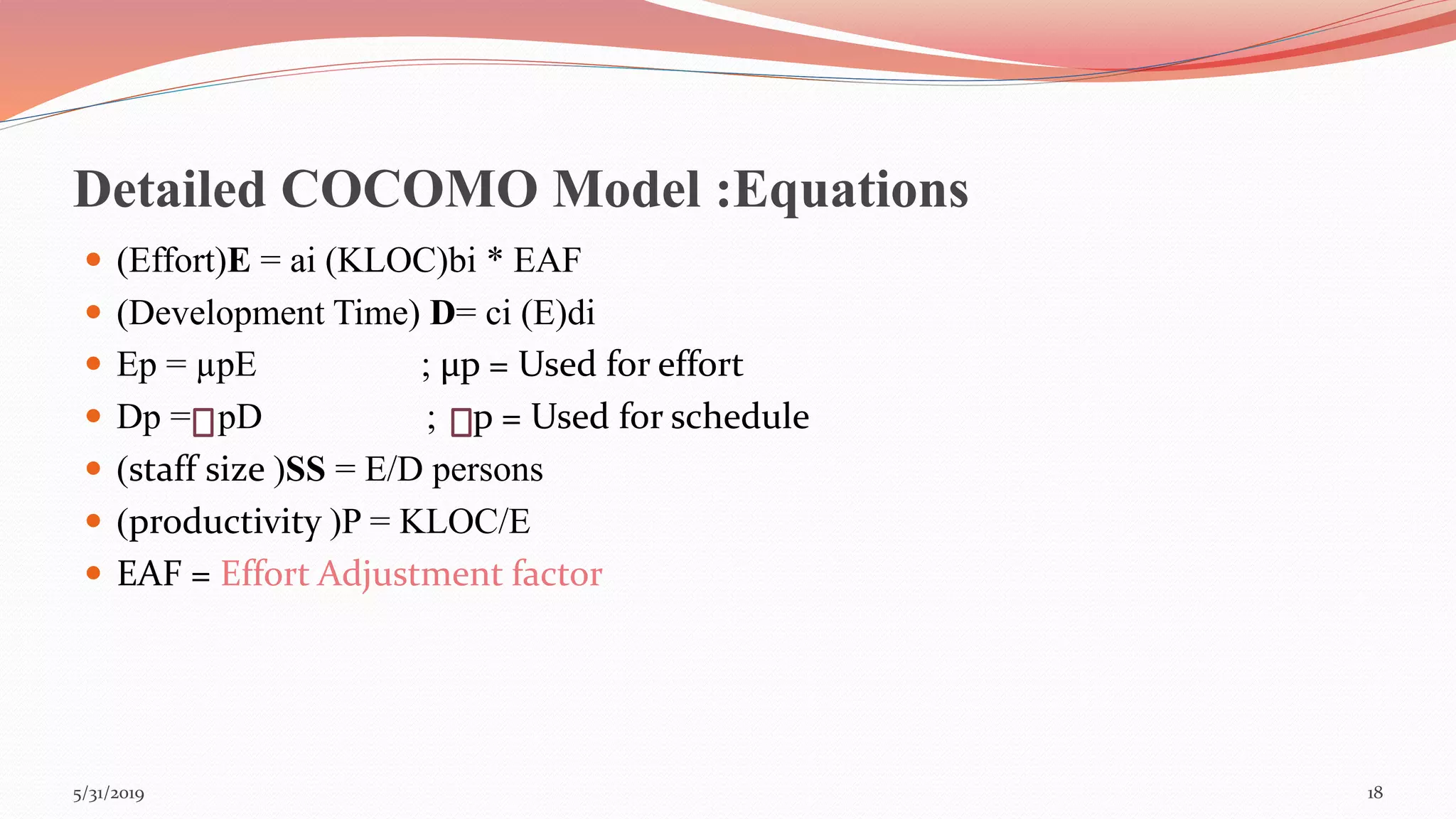
Presented by
Hajra Azam ( 16201519-093)
15/31/2019
Table Of Content
Introduction to COCOMO Model
Key Parameters for testing Quality
Development Modes
Comparison of Three COCOMO modes
COCOMO Models
Advantages and Disadvantages
25/31/2019
Introduction to COCOMO Model
 The COCOMO model is one of the most popular cost estimating model in
software engineering domain which is based upon LOC (Line Of Code).
 COCOMO stands for Constructive Cost Model.
 It is a procedural cost estimate model for software projects.
 It was proposed by Barry Boehm in 1970 and published in 1981 .
 COCOMO predicts the effort and schedule for a software product
development based on inputs related to the size of the software.
35/31/2019
Key Parameters for testing Quality
Effort & Schedule
 Effort: Amount of labor that will be required to complete a
task. It is measured in person-months units.
 Schedule: Amount of time that will be required for the
completion of the job. It is measured in the units of time such
as weeks, months.
45/31/2019
Development Modes
 There are three modes of software development project based on development
complexity.
.Organic Mode
Semidetached Mode
Embedded Mode
55/31/2019
Organic Mode
 Relatively small, simple software projects .
 problem is well understood and has been solved in the past.
 Relatively small and requires little innovation.
 Team size is small and team members have a good experience.
Semi-detached Mode
 The projects classified as Semi-Detached are comparatively less familiar and difficult to
develop compared to the organic ones.
 Require better guidance and creativity.
 Team size is medium with mixed experience.
65/31/2019
Embedded Mode
 It is combination of organic and semi detach mode.
 A software project with requiring the highest level of complexity, creativity, and
experience requirement fall under this category.
 Such software requires a larger team size than the other two mode.
 Developers need to be sufficiently experienced and creative to develop such
complex models.
75/31/2019
Comparison of Three COCOMO modes
85/31/2019
COCOMO Models
95/31/2019
Basic COCOMO Model
 Basic COCOMO is good for quick, early, rough of software costs.
 It does not account for differences in hardware constraints, Team quality and
experience, use of modern tools and techniques, and other project attributes.
Project estimations:
 Approximate estimate of project parameters(cost , development Time, persons
required to complete a task).
 Software development effort is estimated using LOC(Line Of Code)
105/31/2019
Basic COCOMO Model: Equations
 (Effort applied)E=ab (KLOC) b
b
 (Development Time)D=cb (E) d
b
 (Productivity)P= KLOC/E
 (Staff Size)SS = E/D persons
Where
 KLOC  Kilo Line Of Code(Thousands of line).
 A,b,c,d are coefficients.
115/31/2019
Example
 Suppose that a project was estimated to be 400 KLOC. Calculate the effort and development time for
each of the three modes i.e. organic , semidetached and embedded.
 Solution The basic COCOMO equations take the form: E = ab (KLOC)bb
D = cb (E)db
 Estimated size of the project = 400 KLOC
 1. Organic Mode
 E = 2.4 (400)1.05 = 1295.31
 D = 2.5 (1295.31)0.38 = 38.07
 2. Semi detached Mode
 E = 3.0 (400)1.12 = 2462.79
 D = 2.5 (2462.79)0.35 = 38.45
 3. Embedded Mode
 E = 3.6 (400)1.20 = 4772.81
 D = 2.5 (4772.81)0.32 = 37.59
125/31/2019
Intermediate COCOMO Model
 It is extension of Basic COCOMO model. In the Intermediate model ,additional
set of 15 predictors called cost drivers are introduced.
 It refine estimates obtained by Basic COCOMO model.
 It refines cost estimations using 15 cost drivers.
 Classification of Cost Drivers and their attributes
 The cost drivers are grouped into 4 categories:-
 1.Product attributes
 a. Required software reliability (RELY)
 b. Database size (DATA)
 c. Product complexity (CPLX)
135/31/2019
Classification of Cost Drivers and their attributes(cont’d)
2. Computer attributes
 a. Execution time constraint (TIME)
 b. Main store constraint (STOR)
 c. Virtual machine volatility (VIRT)
 d. Computer turnaround time (TURN)
3. Personnel attributes
 a. Analyst capability (ACAP)
 b. Application experience (AEXP)
 c. Programmer capability (PCAP)
 d. Virtual machine experience (VEXP)
 e. Programming Language experience (LEXP)
4. Project attributes
 a. Modern programming practices (MODP)
 b. Use of software tool (TOOL)
 c. Required development schedule (SCED) 145/31/2019
Intermediate COCOMO Model : Equations
 (Effort)E = ai (KLOC)bi * EAF
 (Development Time)D = ci (E)di
 (Staff Size)SS = E/D persons
 (Productivity)P = KLOC/E
Where EAF  Effort Adjustment Factor
Co- efficients for Intermediate COCOMO
155/31/2019
Detailed COCOMO Model
It refine intermediate COCOMO Model.
In detailed cocomo, the whole software is divided into different modules and then we apply
COCOMO in different modules to estimate effort and then sum the effort.
The Development phases :
 Plan/ requirements: This is the first phase of the development cycle. The requirement is
analyzed, the product plan is set up and a full product specification is generated. This phase
consumes from 6% to 8% of the effort and 10% to 40% of the development time.
 Product Design: The second phase of the COCOMO development cycle is concerned with
the determination of the product architecture and the specification of the subsystem. This
phase requires from 16% to 18% of the nominal effort and can last from 19% to 38% of
the development time.
165/31/2019
Detailed COCOMO Model :Development Phases
 Programming: The third phase of the COCOMO development cycle is divided into
two sub phases: detailed design and code/unit test. This phase requires from 48% to
68% of the effort and lasts from 24% to 64% of the development time.
 Integration/test: This phase of the COCOMO development cycle occurs before
delivery. This mainly consist of putting the tested parts together and then testing the
final product this phase requires from 16% to 34% of the nominal effort and can last
from 18% to 34% of the development time
175/31/2019
Detailed COCOMO Model :Equations
 (Effort)E = ai (KLOC)bi * EAF
 (Development Time) D= ci (E)di
 Ep = µpE ; µp = Used for effort
 Dp = pD ; p = Used for schedule
 (staff size )SS = E/D persons
 (productivity )P = KLOC/E
 EAF = Effort Adjustment factor
185/31/2019
Advantages:
COCOMO is realistic and easy to interpret.
Works on historical data and hence is more predictable and accurate.
The drivers are very helpful to understand the impact on the different factors that
affect the project costs.
Disadvantages:
COCOMO model ignores requirements and all documentation.
It ignores customer skills, cooperation, knowledge and other parameters.
It ignores hardware issues.
It is dependent on the amount of time spent in each phase.
195/31/2019
205/31/2019

COCOMO model

  • 1.
    Presented by Hajra Azam( 16201519-093) 15/31/2019
  • 2.
    Table Of Content Introductionto COCOMO Model Key Parameters for testing Quality Development Modes Comparison of Three COCOMO modes COCOMO Models Advantages and Disadvantages 25/31/2019
  • 3.
    Introduction to COCOMOModel  The COCOMO model is one of the most popular cost estimating model in software engineering domain which is based upon LOC (Line Of Code).  COCOMO stands for Constructive Cost Model.  It is a procedural cost estimate model for software projects.  It was proposed by Barry Boehm in 1970 and published in 1981 .  COCOMO predicts the effort and schedule for a software product development based on inputs related to the size of the software. 35/31/2019
  • 4.
    Key Parameters fortesting Quality Effort & Schedule  Effort: Amount of labor that will be required to complete a task. It is measured in person-months units.  Schedule: Amount of time that will be required for the completion of the job. It is measured in the units of time such as weeks, months. 45/31/2019
  • 5.
    Development Modes  Thereare three modes of software development project based on development complexity. .Organic Mode Semidetached Mode Embedded Mode 55/31/2019
  • 6.
    Organic Mode  Relativelysmall, simple software projects .  problem is well understood and has been solved in the past.  Relatively small and requires little innovation.  Team size is small and team members have a good experience. Semi-detached Mode  The projects classified as Semi-Detached are comparatively less familiar and difficult to develop compared to the organic ones.  Require better guidance and creativity.  Team size is medium with mixed experience. 65/31/2019
  • 7.
    Embedded Mode  Itis combination of organic and semi detach mode.  A software project with requiring the highest level of complexity, creativity, and experience requirement fall under this category.  Such software requires a larger team size than the other two mode.  Developers need to be sufficiently experienced and creative to develop such complex models. 75/31/2019
  • 8.
    Comparison of ThreeCOCOMO modes 85/31/2019
  • 9.
  • 10.
    Basic COCOMO Model Basic COCOMO is good for quick, early, rough of software costs.  It does not account for differences in hardware constraints, Team quality and experience, use of modern tools and techniques, and other project attributes. Project estimations:  Approximate estimate of project parameters(cost , development Time, persons required to complete a task).  Software development effort is estimated using LOC(Line Of Code) 105/31/2019
  • 11.
    Basic COCOMO Model:Equations  (Effort applied)E=ab (KLOC) b b  (Development Time)D=cb (E) d b  (Productivity)P= KLOC/E  (Staff Size)SS = E/D persons Where  KLOC  Kilo Line Of Code(Thousands of line).  A,b,c,d are coefficients. 115/31/2019
  • 12.
    Example  Suppose thata project was estimated to be 400 KLOC. Calculate the effort and development time for each of the three modes i.e. organic , semidetached and embedded.  Solution The basic COCOMO equations take the form: E = ab (KLOC)bb D = cb (E)db  Estimated size of the project = 400 KLOC  1. Organic Mode  E = 2.4 (400)1.05 = 1295.31  D = 2.5 (1295.31)0.38 = 38.07  2. Semi detached Mode  E = 3.0 (400)1.12 = 2462.79  D = 2.5 (2462.79)0.35 = 38.45  3. Embedded Mode  E = 3.6 (400)1.20 = 4772.81  D = 2.5 (4772.81)0.32 = 37.59 125/31/2019
  • 13.
    Intermediate COCOMO Model It is extension of Basic COCOMO model. In the Intermediate model ,additional set of 15 predictors called cost drivers are introduced.  It refine estimates obtained by Basic COCOMO model.  It refines cost estimations using 15 cost drivers.  Classification of Cost Drivers and their attributes  The cost drivers are grouped into 4 categories:-  1.Product attributes  a. Required software reliability (RELY)  b. Database size (DATA)  c. Product complexity (CPLX) 135/31/2019
  • 14.
    Classification of CostDrivers and their attributes(cont’d) 2. Computer attributes  a. Execution time constraint (TIME)  b. Main store constraint (STOR)  c. Virtual machine volatility (VIRT)  d. Computer turnaround time (TURN) 3. Personnel attributes  a. Analyst capability (ACAP)  b. Application experience (AEXP)  c. Programmer capability (PCAP)  d. Virtual machine experience (VEXP)  e. Programming Language experience (LEXP) 4. Project attributes  a. Modern programming practices (MODP)  b. Use of software tool (TOOL)  c. Required development schedule (SCED) 145/31/2019
  • 15.
    Intermediate COCOMO Model: Equations  (Effort)E = ai (KLOC)bi * EAF  (Development Time)D = ci (E)di  (Staff Size)SS = E/D persons  (Productivity)P = KLOC/E Where EAF  Effort Adjustment Factor Co- efficients for Intermediate COCOMO 155/31/2019
  • 16.
    Detailed COCOMO Model Itrefine intermediate COCOMO Model. In detailed cocomo, the whole software is divided into different modules and then we apply COCOMO in different modules to estimate effort and then sum the effort. The Development phases :  Plan/ requirements: This is the first phase of the development cycle. The requirement is analyzed, the product plan is set up and a full product specification is generated. This phase consumes from 6% to 8% of the effort and 10% to 40% of the development time.  Product Design: The second phase of the COCOMO development cycle is concerned with the determination of the product architecture and the specification of the subsystem. This phase requires from 16% to 18% of the nominal effort and can last from 19% to 38% of the development time. 165/31/2019
  • 17.
    Detailed COCOMO Model:Development Phases  Programming: The third phase of the COCOMO development cycle is divided into two sub phases: detailed design and code/unit test. This phase requires from 48% to 68% of the effort and lasts from 24% to 64% of the development time.  Integration/test: This phase of the COCOMO development cycle occurs before delivery. This mainly consist of putting the tested parts together and then testing the final product this phase requires from 16% to 34% of the nominal effort and can last from 18% to 34% of the development time 175/31/2019
  • 18.
    Detailed COCOMO Model:Equations  (Effort)E = ai (KLOC)bi * EAF  (Development Time) D= ci (E)di  Ep = µpE ; µp = Used for effort  Dp = pD ; p = Used for schedule  (staff size )SS = E/D persons  (productivity )P = KLOC/E  EAF = Effort Adjustment factor 185/31/2019
  • 19.
    Advantages: COCOMO is realisticand easy to interpret. Works on historical data and hence is more predictable and accurate. The drivers are very helpful to understand the impact on the different factors that affect the project costs. Disadvantages: COCOMO model ignores requirements and all documentation. It ignores customer skills, cooperation, knowledge and other parameters. It ignores hardware issues. It is dependent on the amount of time spent in each phase. 195/31/2019
  • 20.