This document provides information about a textbook titled "Circuit Analysis II with MATLAB® Applications" by Steven T. Karris. The textbook covers advanced electrical engineering concepts like second order circuits, resonance, Laplace transforms, frequency response, transformers, and more. It includes examples and instructions for using MATLAB to obtain solutions. Steven Karris has over 30 years of professional engineering experience and 25 years of teaching experience, and founded Orchard Publications which published this textbook.

1. Orchard Publications, Fremont, California
www.orchardpublications.com
num=[0 1100 0]; den=[1 1100 10^5]; w=logspace(0,5,100); bode(num,den,w); grid
Steven T. Karris
Circuit Analysis II
with MATLAB® Applications

2. Circuit Analysis II
with MATLAB® Applications
Students and working professionals will find Circuit
Analysis II with MATLAB® Applications to be a con-
cise and easy-to-learn text. It provides complete,
clear, and detailed explanations of advanced electri-
cal engineering concepts illustrated with numerous
practical examples.
This text includes the following chapters and appendices:
• Second Order Circuits • Resonance • Elementary Signals • The Laplace Transformation
• The Inverse Laplace Transformation • Circuit Analysis with Laplace Transforms • Frequency
Response and Bode Plots • Self and Mutual Inductances - Transformers • One and Two Port
Networks • Three Phase Systems • Introduction to MATLAB • Differential Equations • Matrices
and Determinants • Constructing Semilog Plots with Microsoft Excel • Scaling
Each chapter contains numerous practical applications supplemented with detailed instructions
for using MATLAB to obtain quick and accurate answers.
Steven T. Karris is the president and founder of Orchard Publications. He earned a bachelors
degree in electrical engineering at Christian Brothers University, Memphis, Tennessee, a masters
degree in electrical engineering at Florida Institute of Technology, Melbourne, Florida, and has
done post-master work at the latter. He is a registered professional engineer in California and
Florida. He has over 30 years of professional engineering experience in industry. In addition, he
has over 25 years of teaching experience that he acquired at several educational institutions as
an adjunct professor. He is currently with UC Berkeley Extension.
Orchard Publications, Fremont, California
Visit us on the Internet
www.orchardpublications.com
or email us: info@orchardpublications.com
ISBN 0-9709511-9-1
$39.95 U.S.A.

3. Circuit Analysis II
with MATLAB® Applications
Steven T. Karris
Orchard Publications
www.orchardpublications.com

4. Circuit Analysis II with MATLAB® Applications
Copyright 2003 Orchard Publications. All rights reserved. Printed in Canada. No part of this publication may be
reproduced or distributed in any form or by any means, or stored in a data base or retrieval system, without the prior
written permission of the publisher.
Direct all inquiries to Orchard Publications, 39510 Paseo Padre Parkway, Fremont, California 94538, U.S.A.
URL: http://www.orchardpublications.com
Product and corporate names are trademarks or registered trademarks of the MathWorks , Inc., and Microsoft
Corporation. They are used only for identification and explanation, without intent to infringe.
Library of Congress Cataloging-in-Publication Data
Library of Congress Control Number: 2003094467
Copyright Number TX-745-064
ISBN 0-9709511-9-1
Disclaimer
The publisher has used his best effort to prepare this text. However, the publisher and author makes no warranty of any
kind, expressed or implied with regard to the accuracy, completeness, and computer codes contained in this book, and
shall not be liable in any event for incidental or consequential damages in connection with, or arising out of, the
performance or use of these programs.
This book was created electronically using Adobe Framemaker .

5. Circuit Analysis II with MATLAB Applications
Orchard Publications
Preface
This text is written for use in a second course in circuit analysis. The reader of this book should have
the traditional undergraduate knowledge of an introductory circuit analysis material such as Circuit
Analysis I with MATLAB® Applications by this author. Another prerequisite would be knowledge of
differential equations, and in most cases, engineering students at this level have taken all required
mathematics courses. It encompasses a spectrum of subjects ranging from the most abstract to the
most practical, and the material can be covered in one semester or two quarters. Appendix B serves as
a review of differential equations with emphasis on engineering related topics and it is recommended
for readers who may need a review of this subject.
There are several textbooks on the subject that have been used for years. The material of this book is
not new, and this author claims no originality of its content. This book was written to fit the needs of
the average student. Moreover, it is not restricted to computer oriented circuit analysis. While it is true
that there is a great demand for electrical and computer engineers, especially in the internet field, the
demand also exists for power engineers to work in electric utility companies, and facility engineers to
work in the industrial areas.
Chapter 1 is an introduction to second order circuits and it is essentially a sequel to first order circuits
that were discussed in the last chapter of as Circuit Analysis I with MATLAB® Applications. Chapter 2
is devoted to resonance, and Chapter 3 presents practical methods of expressing signals in terms of
the elementary functions, i.e., unit step, unit ramp, and unit impulse functions. Thus, any signal can be
represented in the compex frequency domain using the Laplace transformation.
Chapters 4 and 5 are introductions to the unilateral Laplace transform and Inverse Laplace transform
respectively, while Chapter 6 presents several examples of analyzing electric circuits using Laplace
transformation methods. Chapter 7 begins with the frequency response concept and Bode magnitude
and frequency plots. Chapter 8 is devoted to transformers with an introduction to self and mutual
inductances. Chapter 9 is an introduction to one- and two-terminal devices and presents several
practical examples. Chapter 10 is an introduction to three-phase circuits.
It is not necessary that the reader has previous knowledge of MATLAB®. The material of this text
can be learned without MATLAB. However, this author highly recommends that the reader studies
this material in conjunction with the inexpensive MATLAB Student Version package that is available
at most college and university bookstores. Appendix A of this text provides a practical introduction
to MATLAB. As shown on the front cover of this text the magnitude and phase plots can be easily
obtained with a one line MATLAB code. Moreover, MATLAB will be invaluable in later studies such
as the design of analog and digital filters.

6. Circuit Analysis II with MATLAB Applications
Orchard Publications
As stated above, Appendix B is a review of differential equations. Appendix C is an introduction
to matrices, Appendix D provides instructions on constructing semilog templates to be used with
Bode plots, and Appendix E discusses scaling methods.
In addition to numerous real-world examples, this text contains several exercises at the end of
each chapter. Detailed solutions of all exercises are provided at the end of each chapter. The
rationale is to encourage the reader to solve all exercises and check his effort for correct solutions
and appropriate steps in obtaining the correct solution. And since this text was written to serve as
a self-study or supplementary textbook, it provides the reader with a resource to test his
knowledge.
The author has accumulated many additional problems for homework assignment and these are
available to those instructors who adopt this text either as primary or supplementary text, and
prefer to assign problems without the solutions. He also has accumulated many sample exams.
The author is indebted to the class of the Spring semester of 2001 at San Jose State University,
San Jose, California, for providing several of the examples and exercises of this text.
Like any other new book, this text may contain some grammar and typographical errors.
Accordingly, all feedback for errors, advice, and comments will be most welcomed and greatly
appreciated.
Orchard Publications
info@orchardpublications.com

7. Circuit Analysis II with MATLAB Applications i
Orchard Publications
Contents
Chapter 1
Second Order Circuits
The Response of a Second Order Circuit ....................................................................................1-1
The Series RLC Circuit with DC Excitation ...............................................................................1-2
Response of Series RLC Circuits with DC Excitation ................................................................1-5
Response of Series RLC Circuits with AC Excitation ..............................................................1-11
The Parallel GLC Circuit...........................................................................................................1-14
Response of Parallel GLC Circuits with DC Excitation............................................................1-16
Response of Parallel GLC Circuits with AC Excitation............................................................1-26
Other Second Order Circuits .....................................................................................................1-29
Summary....................................................................................................................................1-36
Exercises....................................................................................................................................1-38
Solutions to Exercises................................................................................................................1-40
Chapter 2
Resonance
Series Resonance.........................................................................................................................2-1
Quality Factor Q0s in Series Resonance.......................................................................................2-4
Parallel Resonance.......................................................................................................................2-6
Quality Factor Q0p in Parallel Resonance....................................................................................2-9
General Definition of Q.............................................................................................................2-10
Energy in L and C at Resonance ...............................................................................................2-11
Half-Power Frequencies - Bandwidth .......................................................................................2-12
A Practical Parallel Resonant Circuit........................................................................................2-16
Radio and Television Receivers ................................................................................................2-17
Summary....................................................................................................................................2-20
Exercises....................................................................................................................................2-22
Solutions to Exercises................................................................................................................2-24
Chapter 3
Elementary Signals
Signals Described in Math Form.................................................................................................3-1
The Unit Step Function ...............................................................................................................3-2
The Unit Ramp Function...........................................................................................................3-10

8. ii Circuit Analysis II with MATLAB Applications
Orchard Publications
The Delta Function....................................................................................................................3-12
Sampling Property of the Delta Function..................................................................................3-12
Sifting Property of the Delta Function ......................................................................................3-13
Higher Order Delta Functions ...................................................................................................3-15
Summary....................................................................................................................................3-19
Exercises....................................................................................................................................3-20
Solutions to Exercises................................................................................................................3-21
Chapter 4
The Laplace Transformation
Definition of the Laplace Transformation...................................................................................4-1
Properties of the Laplace Transform ...........................................................................................4-2
The Laplace Transform of Common Functions of Time...........................................................4-12
The Laplace Transform of Common Waveforms......................................................................4-23
Summary....................................................................................................................................4-29
Exercises....................................................................................................................................4-34
Solutions to Exercises................................................................................................................4-37
Chapter 5
The Inverse Laplace Transformation
The Inverse Laplace Transform Integral .....................................................................................5-1
Partial Fraction Expansion...........................................................................................................5-1
Case for m n............................................................................................................................5-13
Alternate Method of Partial Fraction Expansion.......................................................................5-15
Summary....................................................................................................................................5-18
Exercises....................................................................................................................................5-20
Solutions to Exercises................................................................................................................5-22
Chapter 6
Circuit Analysis with Laplace Transforms
Circuit Transformation from Time to Complex Frequency ........................................................6-1
Complex Impedance Z(s) ............................................................................................................6-8
Complex Admittance Y(s).........................................................................................................6-10
Transfer Functions.....................................................................................................................6-13
Summary....................................................................................................................................6-17
Exercises....................................................................................................................................6-18
Solutions to Exercises................................................................................................................6-21

9. Circuit Analysis II with MATLAB Applications iii
Orchard Publications
Chapter 7
Frequency Response and Bode Plots
Decibel.............................................................................................................................................................7-1
Bandwidth and Frequency Response..........................................................................................................7-3
Octave and Decade........................................................................................................................................7-4
Bode Plot Scales and Asymptotic Approximations ..................................................................................7-5
Construction of Bode Plots when the Zeros and Poles are Real............................................................7-6
Construction of Bode Plots when the Zeros and Poles are Complex.................................................7-12
Corrected Amplitude Plots.........................................................................................................................7-25
Summary........................................................................................................................................................7-36
Exercises........................................................................................................................................................7-38
Solutions to Exercises..................................................................................................................................7-39
Chapter 8
Self and Mutual Inductances - Transformers
Self-Inductance ............................................................................................................................8-1
The Nature of Inductance ............................................................................................................8-1
Lenz’s Law ..................................................................................................................................8-3
Mutually Coupled Coils...............................................................................................................8-3
Establishing Polarity Markings..................................................................................................8-11
Energy Stored in a Pair of Mutually Coupled Inductors ...........................................................8-14
Circuits with Linear Transformers.............................................................................................8-20
Reflected Impedance in Transformers.......................................................................................8-25
The Ideal Transformer ...............................................................................................................8-28
Impedance Matching..................................................................................................................8-32
A Simplified Transformer Equivalent Circuit ...........................................................................8-33
Thevenin Equivalent Circuit......................................................................................................8-34
Summary....................................................................................................................................8-38
Exercises ....................................................................................................................................8-42
Solutions to Exercises................................................................................................................8-44
Chapter 9
One- and Two-port Networks
Introduction and Definitions .......................................................................................................................9-1
One-port Driving-point and Transfer Admittances .................................................................................9-2
One-port Driving-point and Transfer Impedances ..................................................................................9-7
Two-Port Networks.....................................................................................................................................9-12

10. iv Circuit Analysis II with MATLAB Applications
Orchard Publications
The y Parameters..........................................................................................................................................9-12
The z parameters..........................................................................................................................................9-19
The h Parameters.........................................................................................................................................9-24
The g Parameters .........................................................................................................................................9-29
Reciprocal Two-Port Networks.................................................................................................................9-34
Summary........................................................................................................................................................9-38
Exercises........................................................................................................................................................9-43
Solutions to Exercises .................................................................................................................................9-45
Chapter 10
Three-Phase Systems
Advantages of Three-Phase Systems.........................................................................................10-1
Three-Phase Connections ..........................................................................................................10-1
Transformer Connections in Three-Phase Systems...................................................................10-4
Line-to-Line and Line-to-Neutral Voltages and Currents .........................................................10-5
Equivalent Y and Loads .......................................................................................................10-10
Computation by Reduction to Single Phase ............................................................................10-20
Three-Phase Power..................................................................................................................10-21
Instantaneous Power in Three-Phase Systems.........................................................................10-23
Measuring Three-Phase Power................................................................................................10-27
Summary..................................................................................................................................10-30
Exercises..................................................................................................................................10-32
Solutions to Exercises..............................................................................................................10-33
Appendix A
Introduction to MATLAB®
MATLAB® and Simulink®.......................................................................................................A-1
Command Window.....................................................................................................................A-1
Roots of Polynomials..................................................................................................................A-3
Polynomial Construction from Known Roots ............................................................................A-4
Evaluation of a Polynomial at Specified Values ........................................................................A-6
Rational Polynomials..................................................................................................................A-8
Using MATLAB to Make Plots................................................................................................A-10
Subplots ....................................................................................................................................A-19
Multiplication, Division and Exponentiation ...........................................................................A-20
Script and Function Files..........................................................................................................A-26
Display Formats........................................................................................................................A-31

11. Circuit Analysis II with MATLAB Applications v
Orchard Publications
Appendix B
Differential Equations
Simple Differential Equations ....................................................................................................B-1
Classification ..............................................................................................................................B-3
Solutions of Ordinary Differential Equations (ODE).................................................................B-6
Solution of the Homogeneous ODE ...........................................................................................B-8
Using the Method of Undetermined Coefficients for the Forced Response.............................B-10
Using the Method of Variation of Parameters for the Forced Response..................................B-20
Exercises ...................................................................................................................................B-24
Appendix C
Matrices and Determinants
Matrix Definition ........................................................................................................................C-1
Matrix Operations.......................................................................................................................C-2
Special Forms of Matrices ..........................................................................................................C-5
Determinants...............................................................................................................................C-9
Minors and Cofactors................................................................................................................C-12
Cramer’s Rule...........................................................................................................................C-16
Gaussian Elimination Method ..................................................................................................C-19
The Adjoint of a Matrix............................................................................................................C-20
Singular and Non-Singular Matrices ........................................................................................C-21
The Inverse of a Matrix ............................................................................................................C-21
Solution of Simultaneous Equations with Matrices..................................................................C-23
Exercises ...................................................................................................................................C-30
Appendix D
Constructing Semilog Plots with Microsoft Excel
The Excel Spreadsheet Window.................................................................................................D-1
Instructions for Constructing Semilog Plots...............................................................................D-2
Appendix E
Scaling
Magnitude Scaling ...................................................................................................................... E-1
Frequency Scaling....................................................................................................................... E-1
Exercises ..................................................................................................................................... E-8
Solutions to Exercises................................................................................................................. E-9

12. vi Circuit Analysis II with MATLAB Applications
Orchard Publications
NOTES

13. Circuit Analysis II with MATLAB Applications 1-1
Orchard Publications
Chapter 1
Second Order Circuits
his chapter discusses the natural, forced and total responses in circuits containing resistors,
inductors and capacitors. These circuits are characterized by linear second-order differential
equations whose solutions consist of the natural and the forced responses. We will consider
both DC (constant) and AC (sinusoidal) excitations.
1.1 The Response of a Second Order Circuit
A circuit containing energy storage devices (inductors and capacitors) is said to be an nth-order cir-
cuit, and the differential equation describing the circuit is an nth-order differential equation. For exam-
ple, if a circuit contains an inductor and a capacitor, or two capacitors or two inductors, along with
other devices such as resistors, it is said to be a second-order circuit and the differential equation that
describes it is a second order differential equation. It is possible, however, to describe a circuit having
two energy storage devices with a set of two first-order differential equations, a circuit which has
three energy storage devices with a set of three first-order differential equations and so on. These are
called state equations*
but these will not be discussed here.
The response is found from the differential equation describing the circuit, and its solution is
obtained as follows:
1. We write the differential or integrodifferential (nodal or mesh) equation describing the circuit. We
differentiate, if necessary, to eliminate the integral.
2. We obtain the forced (steady-state) response. Since the excitation in our work here will be either a
constant (DC) or sinusoidal (AC) in nature, we expect the forced response to have the same form
as the excitation. We evaluate the constants of the forced response by substitution of the assumed
forced response into the differential equation and equate terms of the left side with the right side.
Refer to Appendix B for the general expression of the forced response (particular solution).
3. We obtain the general form of the natural response by setting the right side of the differential
equation equal to zero, in other words, solve the homogeneous differential equation using the
characteristic equation.
4. Add the forced and natural responses to form the complete response.
5. We evaluate the constants of the complete response from the initial conditions.
* State variables and state equations are discussed in Signals and Systems with MATLAB Applications, ISBN 0-
9709511-3-2 by this author.
T
n

14. Chapter 1 Second Order Circuits
1-2 Circuit Analysis II with MATLAB Applications
Orchard Publications
1.2 The Series RLC Circuit with DC Excitation
Let us consider the series circuit of Figure 1.1 where the initial conditions are ,
, and is the unit step function.*
We want to find an expression for the current
for .
Figure 1.1. Series RLC Circuit
For this circuit
(1.1)
and by differentiation
To find the forced response, we must first specify the nature of the excitation , that is, DC or AC.
If is DC ( =constant), the right side of (1.1) will be zero and thus the forced response compo-
nent . If is AC ( , the right side of (1.1) will be another sinusoid and
therefore . Since in this section we are concerned with DC excitations, the right
side will be zero and thus the total response will be just the natural response.
The natural response is found from the homogeneous equation of (1.1), that is,
(1.2)
The characteristic equation of (1.2) is
* The unit step function is discussed in detail in Chapter 3. For our present discussion it will suffice to state that
for and for .
RLC iL 0 I0=
vC 0 V0= u0 t i t
u0 t 0= t 0 u0 t 1= t 0
t 0
+
vS u0 t
i t
R
L
C
Ri L
di
dt
-----
1
C
---- i td
0
t
V0+ + + vS= t 0
R
di
dt
----- L
d
2
i
dt
2
------- i
C
----+ +
dvS
dt
--------= t 0
vS
vS vS
if 0= vS vS V t +cos=
if I t +cos=
R
di
dt
----- L
d
2
i
dt
2
------- i
C
----+ + 0=
Ls
2
Rs
1
C
----+ + 0=

15. 1-3 Circuit Analysis II with MATLAB Applications
Orchard Publications
The Series RLC Circuit with DC Excitation
or
from which
(1.3)
We will use the following notations:
(1.4)
where the subscript stands for series circuit. Then, we can express (1.3) as
(1.5)
or
(1.6)
Case I: If , the roots and are real, negative, and unequal. This results in the over-
damped natural response and has the form
(1.7)
Case II: If , the roots and are real, negative, and equal. This results in the critically
damped natural response and has the form
(1.8)
Case III: If , the roots and are complex conjugates. This is known as the underdamped
or oscillatory natural response and has the form
(1.9)
A typical overdamped response is shown in Figure 1.2 where it is assumed that . This plot
was created with the following MATLAB code:
s
2 R
L
---s 1
LC
-------+ + 0=
s1 s2
R
2L
------–
R
2
4L
2
--------
1
LC
-------–=
S
R
2L
------=
or Damping
Coefficient
0
1
LC
-----------=
Resonant
Frequency
S S
2
0
2
–=
Beta
Coefficient
nS 0
2
S
2
–=
Damped Natural
Frequency
s
s1 s2 S– S
2
0
2
– S– S if S
2
0
2
= =
s1 s2 S– 0
2
S
2
– S– nS
if 0
2
S
2
= =
S
2
0
2
s1 s2
in t k1e
s1t
k2e
s2t
+=
S
2
0
2
= s1 s2
in t e
St–
k1 k2t+=
0
2
S
2
s1 s2
in t e
S t–
k1 nS
cos t k2 nS
tsin+ k3e
St–
nS
cos t += =
in 0 0=

16. Chapter 1 Second Order Circuits
1-4 Circuit Analysis II with MATLAB Applications
Orchard Publications
t=0: 0.01: 6; ft=8.4.*(exp( t)-exp( 6.*t)); plot(t,ft); grid; xlabel('t');...
ylabel('f(t)'); title('Overdamped Response for 4.8.*(exp( t) exp( 6.*t))')
Figure 1.2. Typical overdamped response
A typical critically damped response is shown in Figure 1.3 where it is assumed that . This
plot was created with the following MATLAB code:
t=0: 0.01: 6; ft=420.*t.*(exp( 2.45.*t)); plot(t,ft); grid; xlabel('t');...
ylabel('f(t)'); title('Critically Damped Response for 420.*t.*(exp( 2.45.*t))')
Figure 1.3. Typical critically damped response
A typical underdamped response is shown in Figure 1.4 where it is assumed that . This
plot was created with the following MATLAB code:
in 0 0=
in 0 0=

17. 1-5 Circuit Analysis II with MATLAB Applications
Orchard Publications
Response of Series RLC Circuits with DC Excitation
t=0: 0.01: 10; ft=210.*sqrt(2).*(exp( 0.5.*t)).*sin(sqrt(2).*t); plot(t,ft); grid; xlabel('t');...
ylabel('f(t)'); title('Underdamped Response for 210.*sqrt(2).*(exp( 0.5.*t)).*sin(sqrt(2).*t)')
Figure 1.4. Typical underdamped response
1.3 Response of Series RLC Circuits with DC Excitation
Depending on the circuit constants , , and , the total response of a series circuit that is
excited by a DC source, may be overdamped, critically damped, or underdamped. In this section we
will derive the total response of series circuits that are excited by DC sources.
Example 1.1
For the circuit of Figure 1.5, , , and the resistor represents the
resistance of the inductor. Compute and sketch for .
Figure 1.5. Circuit for Example 1.1
Solution:
This circuit can be represented by the integrodifferential equation
R L C RLC
RLC
iL 0 5 A= vC 0 2.5 V= 0.5
i t t 0
+
15u0 t V
i t
0.5
1 mH
100 6 mF

18. Chapter 1 Second Order Circuits
1-6 Circuit Analysis II with MATLAB Applications
Orchard Publications
(1.10)
Differentiating and noting that the derivatives of the constants and are zero, we obtain the
homogeneous differential equation
or
and by substitution of the known values , , and
(1.11)
The roots of the characteristic equation of (1.11) are and . The total response
is just the natural response and for this example it is overdamped. Therefore, from (1.7),
(1.12)
The constants and can be evaluated from the initial conditions. Thus from the first initial con-
dition and (1.12) we get
(1.13)
We need another equation in order to compute the values of and . With this equation we will
make use of the second initial condition, that is, . Since , we dif-
ferentiate (1.12), we evaluate it at , and we equate it with this initial condition. Then,
(1.14)
Also, at ,
Ri L
di
dt
-----
1
C
---- i td
0
t
vC 0+ + + 15= t 0
vC 0 15
R
di
dt
----- L
d
2
i
dt
2
------- i
C
----+ + 0=
d
2
i
dt
2
-------
R
L
---
di
dt
----- i
LC
-------+ + 0=
R L C
d
2
i
dt
2
------- 500
di
dt
----- 60000i+ + 0=
s1 200–= s2 300–=
i t in t k1e
s1t
k2e
s2t
+ k1e
200– t
k2e
300– t
+= ==
k1 k2
iL 0 i 0 5 A= =
i 0 k1e
0
k2e
0
+ 5= =
k1 k2+ 5=
k1 k2
vC 0 2.5 V= iC t i t C
dvC
dt
--------= =
t 0
+
=
di
dt
----- 200k– 1e
200– t
300k2– e
300– t
and=
di
dt
-----
t 0
+
=
200k– 1 300– k2=
t 0
+
=
Ri 0
+
L
di
dt
-----
t 0
+
=
vc 0
+
+ + 15=

19. 1-7 Circuit Analysis II with MATLAB Applications
Orchard Publications
Response of Series RLC Circuits with DC Excitation
and solving for we get
(1.15)
Next, equating (1.14) with (1.15) we get:
(1.16)
Simultaneous solution of (1.13) and (1.16) yields and . By substitution into (1.12)
we find the total response as
(1.17)
Check with MATLAB:
syms t; % Define symbolic variable t
R=0.5; L=10^( 3); C=100*10^( 3)/6;% Circuit constants
y0=115*exp( 200*t) 110*exp(-300*t); % Let solution i(t)=y0
y1=diff(y0); % Compute the first derivative of y0, i.e., di/dt
y2=diff(y0,2); % Compute the second derivative of y0, i.e, di2/dt2
% Substitute the solution i(t), i.e., equ (1.17)
% into differential equation of (1.11) to verify
% that correct solution was obtained.
% We must also verify that the initial
% conditions are satisfied
y=y2+500*y1+60000*y0;
i0=115*exp( 200*0) 110*exp( 300*0);
vC0= R*i0 L*( 23000*exp( 200*0)+33000*exp( 300*0))+15;
fprintf(' n');...
disp('Solution was entered as y0 = '); disp(y0);...
disp('1st derivative of solution is y1 = '); disp(y1);...
disp('2nd derivative of solution is y2 = '); disp(y2);...
disp('Differential equation is satisfied since y = y2+y1+y0 = '); disp(y);...
disp('1st initial condition is satisfied since at t = 0, i0 = '); disp(i0);...
disp('2nd initial condition is also satisfied since vC+vL+vR=15 and vC0 = ');...
disp(vC0);...
fprintf(' n')
Solution was entered as y0 =
115*exp(-200*t)-110*exp(-300*t)
di
dt
-----
t 0
+
=
di
dt
-----
t 0
+
=
15 0.5 5– 2.5–
10
3–
--------------------------------------- 10000= =
200k– 1 300– k2 10000=
k– 1 1.5– k2 50=
k1 115= k2 110–=
i t in t 115e
200– t
110– e
300– t
==

20. Chapter 1 Second Order Circuits
1-8 Circuit Analysis II with MATLAB Applications
Orchard Publications
1st derivative of solution is y1 =
-23000*exp(-200*t)+33000*exp(-300*t)
2nd derivative of solution is y2 =
4600000*exp(-200*t)-9900000*exp(-300*t)
Differential equation is satisfied since y = y2+y1+y0 = 0
1st initial condition is satisfied since at t = 0, i0 = 5
2nd initial condition is also satisfied since vC+vL+vR=15 and vC0
= 2.5000
We will use the following MATLAB code to sketch .
t=0: 0.0001: 0.025; i1=115.*(exp( 200.*t)); i2=110.*(exp( 300.*t)); iT=i1 i2;...
plot(t,i1,t,i2,t,iT); grid; xlabel('t'); ylabel('i1, i2, iT'); title('Response iT for Example 1.1')
Figure 1.6. Plot for of Example 1.1
In the above example, differentiation eliminated (set equal to zero) the right side of the differential
equation and thus the total response was just the natural response. A different approach however,
may not set the right side equal to zero, and therefore the total response will contain both the natural
and forced components. To illustrate, we will use the following approach.
The capacitor voltage, for all time , may be expressed as and as before, the circuit
can be represented by the integrodifferential equation
(1.18)
i t
i t
t vC t
1
C
---- i td
–
t
=
Ri L
di
dt
----- 1
C
---- i td
–
t
+ + 15= u0 t

21. 1-9 Circuit Analysis II with MATLAB Applications
Orchard Publications
Response of Series RLC Circuits with DC Excitation
and since
we rewrite (1.18) as
(1.19)
We observe that this is a non-homogeneous differential equation whose solution will have both the
natural and the forced response components. Of course, the solution of (1.19) will give us the capaci-
tor voltage . This presents no problem since we can obtain the current by differentiation of the
expression for .
Substitution of the given values into (1.19) yields
or
(1.20)
The characteristic equation of (1.20) is the same as of that of (1.11) and thus the natural response is
(1.21)
Since the right side of (1.20) is a constant, the forced response will also be a constant and we denote it
as . By substitution into (1.20) we get
or
(1.22)
The total solution then is the summation of (1.21) and (1.22), that is,
(1.23)
As before, the constants and will be evaluated from the initial conditions. First, using
and evaluating (1.23) at , we get
or
i iC C
dvC
dt
--------= =
RC
dvC
dt
--------- LC
dvC
2
dt
2
--------- vC+ + 15= u0 t
vC t
vC t
50
6
------ 10
3– dvC
dt
-------- 1 10
3– 100
6
---------10
3– dvC
2
dt
2
-------- vC+ + 15= u0 t
dvC
2
dt
2
-------- 500
dvC
dt
-------- 60000vC+ + 9 10
5
= u0 t
vCn t k1e
s1t
k2e
s2t
+ k1e
200– t
k2e
300– t
+= =
vCf k3=
0 0 60000k3+ + 900000=
vCf k3 15= =
vC t vCn t vCf+= k1e
200– t
k2e
300– t
15+ +=
k1 k2
vC 0 2.5 V= t 0=
vC 0 k1e
0
k2e
0
15+ + 2.5= =

22. Chapter 1 Second Order Circuits
1-10 Circuit Analysis II with MATLAB Applications
Orchard Publications
(1.24)
Also,
(1.25)
Next, we differentiate (1.23), we evaluate it at and equate it with (1.25). Then,
(1.26)
Equating the right sides of (1.25) and (1.26) we get
or
(1.27)
From (1.24) and (1.27), we get and . By substitution into (1.23), we obtain the
total solution as
(1.28)
Check with MATLAB:
syms t % Define symbolic variable t
y0=22*exp( 300*t) 34.5*exp( 200*t)+15; % The total solution y(t)
y1=diff(y0) % The first derivative of y(t)
y1 =
-6600*exp(-300*t)+6900*exp(-200*t)
y2=diff(y0,2) % The second derivative of y(t)
y2 =
1980000*exp(-300*t)-1380000*exp(-200*t)
y=y2+500*y1+60000*y0 % Summation of y and its derivatives
y =
900000
Using the expression for we can find the current as
(1.29)
k1 k2+ 12.5–=
iL iC C
dvC
dt
--------= =
dvC
dt
--------
iL
C
---- and
dvC
dt
--------
t 0=
iL 0
C
------------ 5
100
6
--------- 10
3–
------------------------- 300= = ==
t 0=
dvC
dt
-------- 200k1– e
200– t
300k2– e
300– t
and
dvC
dt
--------
t 0=
200k1– 300k2–==
200k1– 300k2– 300=
k1– 1.5k2– 1.5=
k1 34.5–= k2 22=
vC t 22e
300– t
34.5– e
200– t
15+ u0 t=
vC t
i iL= iC C
dvC
dt
--------
100
6
--------- 10
3–
6900e
200t–
6600– e
300t–
115e
200t–
110– e
300t–
A= == =

23. 1-11 Circuit Analysis II with MATLAB Applications
Orchard Publications
Response of Series RLC Circuits with AC Excitation
We observe that (1.29) is the same as (1.17).
We will use the following MATLAB code to sketch .
t=0: 0.001: 0.03; vc1=22.*(exp( 300.*t)); vc2= 34.5.*(exp( 200.*t)); vc3=15;...
vcT=vc1+vc2+vc3; plot(t,vc1,t,vc2,t,vc3,t,vcT); grid; xlabel('t');...
ylabel('vc1, vc2, vc3, vcT'); title('Response vcT for Example 1.1')
Figure 1.7. Plot for of Example 1.1
1.4 Response of Series RLC Circuits with AC Excitation
The total response of a series RLC circuit, which is excited by a sinusoidal source, will also consist of
the natural and forced response components. As we found in the previous section, the natural
response can be overdamped, or critically damped, or underdamped. The forced component will be a
sinusoid of the same frequency as that of the excitation, and since it represents the AC steady-state
condition, we can use phasor analysis to find it. The following example illustrates the procedure.
Example 1.2
For the circuit of Figure 1.8, , , and the resistor represents the
resistance of the inductor. Compute and sketch for .
Solution:
This circuit is the same as that of Example 1.1 except that the circuit is excited by a sinusoidal source;
therefore it can be represented by the integrodifferential equation
(1.30)
i t
vC t
iL 0 5 A= vC 0 2.5 V= 0.5
i t t 0
Ri L
di
dt
-----
1
C
---- i td
0
t
vC 0+ + + 200 10000tcos= t 0

24. Chapter 1 Second Order Circuits
1-12 Circuit Analysis II with MATLAB Applications
Orchard Publications
Figure 1.8. Circuit for Example 1.2
whose solution consists of the summation of the natural and forced responses. We know its natural
response from the previous example. We start with
(1.31)
where the constants and will be evaluated from the initial conditions after has been
found. The steady state (or forced) response will have the form in the
time domain ( -domain) and has the form in the frequency domain ( -domain).
To find we will use the phasor analysis relation where is the phasor current, is
the phasor voltage, and is the impedance of the phasor circuit which, as we know, is
(1.32)
The inductive and capacitive reactances are
and
Then,
Also,
and this yields . Then, by substitution into (1.32),
and thus
+
200 10000tcos u0 t V
i t
0.5
1 mH
100 6 mF
i t in t if t+ k1 e
200– t
k2 e
300– t
if t+ +==
k1 k2 if t
if t k3 10 000t +cos=
t k3 j
if t I V Z= I V
Z
Z R j L 1 C–+ R
2
L 1 C–
2
+ L 1 C– R
1–
tan= =
XL L 10
4
10
3–
10= = =
XC
1
C
--------
1
10
4
100 6 10
3–
--------------------------------------------- 6 10
3–
= = =
R
2
0.5
2
0.25 and L 1 C–
2
10 6 10
3–
–
2
99.88= == =
L 1 C– R
1–
tan 10 6 10
3–
–
0.5
------------------------------------
1–
tan
9.994
0.5
-------------
1–
tan= =
1.52 rads 87.15= =
Z 0.25 99.88+
o
10 87.15
o
= =
I
V
Z
---
200 0
o
10 87.15
o
--------------------------- 20 87.15–
o
= = = 20 10000t 87.15–
o
cos if t=

25. 1-13 Circuit Analysis II with MATLAB Applications
Orchard Publications
Response of Series RLC Circuits with AC Excitation
The total solution is
(1.33)
The constants and are evaluated from the initial conditions. From (1.33) and the first initial
condition we get
(1.34)
We need another equation in order to compute the values of and . This equation will make use
of the second initial condition, that is, . Since , we differentiate
(1.33), we evaluate it at , and we equate it with this initial condition. Then,
(1.35)
and at ,
(1.36)
Also, at
and solving for we get
(1.37)
Next, equating (1.36) with (1.37) we get
or
(1.38)
i t in t if t+ k1e
200– t
k2e
300– t
20 10000t 87.15–
o
cos+ +==
k1 k2
iL 0 5 A=
i 0 k1e
0
k2e
0
20 87.15–
o
cos+ += 5=
i 0 k1 k2 20 0.05+ += 5=
k1 k2+ 4=
k1 k2
vC 0 2.5 V= iC t i t C
dvC
dt
--------= =
t 0=
di
dt
----- 200k– 1e
200– t
300k2– e
300– t
2 10
5
10000t 87.15–
o
sin–=
t 0=
di
dt
-----
t 0=
200k– 1 300k2– 2 10
6
87.15–
o
sin–= 200k– 1 300k2– 2 10
5
+=
t 0
+
=
Ri 0
+
L
di
dt
-----
t 0
+
=
vc 0
+
+ + 200 0cos 200= =
di
dt
-----
t 0
+
=
di
dt
-----
t 0
+
=
200 0.5 5– 2.5–
10
3–
------------------------------------------ 195000= =
200k– 1 300– k2 5000–=
k1 1.5k2+ 25=

26. Chapter 1 Second Order Circuits
1-14 Circuit Analysis II with MATLAB Applications
Orchard Publications
Simultaneous solution of (1.34) and (1.38) yields and . Then, by substitution into
(1.31), the total response is
(1.39)
The plot is shown in Figure 1.9 and was created with the following MATLAB code:
t=0: 0.005: 0.20; i1= 38.*(exp( 200.*t)); i2=42.*(exp( 300.*t));...
i3=20.*cos(10000.*t 87.15.*pi./180); iT=i1+i2+i3; plot(t,i1,t,i2,t,i3,t,iT); grid; xlabel('t');...
ylabel('i1, i2, i3, iT'); title('Response iT for Example 1.2')
Figure 1.9. Plot for of Example 1.2
1.5 The Parallel GLC Circuit
Consider the circuit of Figure 1.10 where the initial conditions are , , and
is the unit step function. We want to find an expression for the voltage for .
Figure 1.10. Parallel RLC circuit
For this circuit
k1 38–= k2 42=
i t 38– e
200– t
42e
300– t
20 10000t 87.15–
o
Acos+ +=
i t
iL 0 I0= vC 0 V0=
u0 t v t t 0
iS u0 t
v t G L C
iCiL
iG

27. 1-15 Circuit Analysis II with MATLAB Applications
Orchard Publications
The Parallel GLC Circuit
or
By differentiation,
(1.40)
To find the forced response, we must first specify the nature of the excitation , that is DC or AC.
If is DC ( =constant), the right side of (1.40) will be zero and thus the forced response compo-
nent . If is AC ( , the right side of (1.40) will be another sinusoid and
therefore . Since in this section we are concerned with DC excitations, the right
side will be zero and thus the total response will be just the natural response.
The natural response is found from the homogeneous equation of (1.40), that is,
(1.41)
whose characteristic equation is
or
from which
(1.42)
and with the following notations,
(1.43)
where the subscript stands for parallel circuit, we can express (1.42) as
iG t iL t iC t+ + iS t=
Gv
1
L
--- v td
0
t
I0+ + C
dv
dt
------+ iS= t 0
C
dv
2
dt
2
-------- G
dv
dt
------ v
L
---+ +
diS
dt
-------= t 0
iS
iS vS
vf 0= iS iS I t +cos=
vf V t +cos=
C
dv
2
dt
2
-------- G
dv
dt
------ v
L
---+ + 0=
Cs
2
Gs
1
L
---+ + 0=
s
2 G
C
----s i
LC
-------+ + 0=
s1 s2
G
2C
-------– G
2
4C
2
--------- 1
LC
-------–=
P
G
2C
-------=
or Damping
Coefficient
0
1
LC
-----------=
Resonant
Frequency
P P
2
0
2
–=
Beta
Coefficient
nP 0
2
P
2
–=
Damped Natural
Frequency
p

28. Chapter 1 Second Order Circuits
1-16 Circuit Analysis II with MATLAB Applications
Orchard Publications
(1.44)
or
(1.45)
Note: From (1.4) and (1.43) we observe that
As in a series circuit, the natural response can be overdamped, critically damped, or under-
damped.
Case I: If , the roots and are real, negative, and unequal. This results in the over-
damped natural response and has the form
(1.46)
Case II: If , the roots and are real, negative, and equal. This results in the critically
damped natural response and has the form
(1.47)
Case III: If , the roots and are complex conjugates. This results in the underdamped
or oscillatory natural response and has the form
(1.48)
1.6 Response of Parallel GLC Circuits with DC Excitation
Depending on the circuit constants (or ), , and , the natural response of a parallel cir-
cuit may be overdamped, critically damped or underdamped. In this section we will derive the total
response of a parallel circuit which is excited by a DC source using the following example.
Example 1.3
For the circuit of Figure 1.11, and . Compute and sketch for .
s1 s2 P– P
2
0
2
– P– P if P
2
0
2
= =
s1 s2 P– 0
2
P
2
– P– nP if 0
2
P
2
= =
S P
vn t
P
2
0
2
s1 s2
vn t k1e
s1t
k2e
s2t
+=
P
2
0
2
= s1 s2
vn t e
P
t–
k1 k2t+=
0
2
P
2
s1 s2
vn t e
Pt–
k1 nPcos t k2 nPtsin+ k3e
Pt–
nPcos t += =
G R L C GLC
GLC
iL 0 2 A= vC 0 5 V= v t t 0

29. 1-17 Circuit Analysis II with MATLAB Applications
Orchard Publications
Response of Parallel GLC Circuits with DC Excitation
Figure 1.11. Circuit for Example 1.3
Solution:
We could write the integrodifferential equation that describes the given circuit, differentiate, and find
the roots of the characteristic equation from the homogeneous differential equation as we did in the
previous section. However, we will skip these steps and start with
(1.49)
and when steady-state conditions have been reached we will have ,
and .
To find out whether the natural response is overdamped, critically damped, or oscillatory, we need to
compute the values of and using (1.43) and the values of and using (1.44) or (1.45).
Then will use (1.46), or (1.47), or (1.48) as appropriate. For this example,
or
and
Then
or and . Therefore, the natural response is overdamped and from (1.46) we get
(1.50)
and the constants and will be evaluated from the initial conditions.
From the initial condition and (1.50) we get
10u0 t A
v t
32 1 640 F
iCiL
iR
10 H
v t vf t vn t+=
v vL L di dt 0= = = vf 0=
v t vn t=
P 0 s1 s2
P
G
2C
-------
1
2RC
-----------
1
2 32 1 640
------------------------------------- 10= = = =
P
2
100=
0
2 1
LC
-------
1
10 1 640
---------------------------- 64= = =
s1 s2 P– P
2
0
2
– 10– 6= =
s1 4–= s2 16–=
v t vn t k1e
s1t
k2e
s2t
+ k1e
4– t
k2e
16– t
+= ==
k1 k2
vC 0 v 0 5 V= =

30. Chapter 1 Second Order Circuits
1-18 Circuit Analysis II with MATLAB Applications
Orchard Publications
or
(1.51)
The second equation that is needed for the computation of the values of and is found from
other initial condition, that is, . Since , we differentiate (1.50),
evaluate it at , and we equate it with this initial condition.Then,
(1.52)
Also, at
and solving for we get
(1.53)
Next, equating (1.52) with (1.53) we get
or
(1.54)
Simultaneous solution of (1.51) and (1.54) yields , , and by substitution
into (1.50) we get the total response as
(1.55)
Check with MATLAB:
syms t % Define symbolic variable t
y0=291*exp( 4*t)/6 261*exp( 16*t)/6; % Let solution v(t) = y0
y1=diff(y0) % Compute and display first derivative
y1 =
-194*exp(-4*t)+696*exp(-16*t)
v 0 k1e
0
k2e
0
+ 5= =
k1 k2+ 5=
k1 k2
iL 0 2 A= iC t C
dvC
dt
-------- C
dv
dt
------= =
t 0
+
=
dv
dt
------ 4k– 1e
4– t
16k2– e
16– t
and=
dv
dt
------
t 0
+
=
4k– 1 16– k2=
t 0
+
=
1
R
---v 0
+
iL 0
+
C
dv
dt
------
t 0
+
=
+ + 10=
dv
dt
------
t 0
+
=
dv
dt
------
t 0
+
=
10 5 32– 2–
1 640
------------------------------- 502= =
4k– 1 16– k2 502=
2k– 1 8– k2 251=
k1 291 6= k2 261– 6=
v t vn t
291
6
---------e
4– t 261
6
---------– e
16– t
==
1
6
--- 291e
4– t
261– e
16– t
V=

31. 1-19 Circuit Analysis II with MATLAB Applications
Orchard Publications
Response of Parallel GLC Circuits with DC Excitation
y2=diff(y0,2) % Compute and display second derivative
y2 =
776*exp(-4*t)-11136*exp(-16*t)
y=y2/640+y1/32+y0/10 % Verify that (1.40) is satisfied
y =
0
The plot is shown in Figure 1.12 where we have used the following MATLAB code:
t=0: 0.01: 1; v1=(291./6).*(exp( 4.*t)); v2= (261./6).*(exp( 16.*t));...
vT=v1+v2; plot(t,v1,t,v2,t,vT); grid; xlabel('t');...
ylabel('v1, v2, vT'); title('Response vT for Example 1.3')
Figure 1.12. Plot for of Example 1.3
From the plot of Figure 1.12, we observe that attains its maximum value somewhere in the inter-
val and sec., and the maximum voltage is approximately . If we desire to compute pre-
cisely the maximum voltage and the exact time it occurs, we can find the derivative of (1.55), set it
equal to zero, and solve for . Thus,
(1.56)
Division of (1.56) by yields
or
v t
v t
0.10 0.12 24 V
t
dv
dt
------
t 0=
1164e
4– t
– 4176e
16– t
+ 0= =
e
16t–
1164e
12t
– 4176+ 0=

32. Chapter 1 Second Order Circuits
1-20 Circuit Analysis II with MATLAB Applications
Orchard Publications
or
and
By substitution into (1.55)
(1.57)
A useful quantity, especially in electronic circuit analysis, is the settling time, denoted as , and it is
defined as the time required for the voltage to drop to of its maximum value. Therefore, is an
indication of the time it takes for to damp-out, meaning to decrease the amplitude of to
approximately zero. For this example, , and we can find by substitution
into (1.55). Then,
(1.58)
and we need to solve for the time . To simplify the computation, we neglect the second term inside
the parentheses of (1.58) since this component of the voltage damps out much faster than the other
component. This expression then simplifies to
or
or
(1.59)
Example 1.4
For the circuit of Figure 1.13, and , and the resistor is to be adjusted so
that the natural response will be critically damped. Compute and sketch for .
e
12t 348
97
---------=
12t
348
97
---------ln= 1.2775=
t tmax
1.2775
12
---------------- 0.106 s= = =
vmax
1
6
--- 291e
4– x0.106
261– e
16– x0.106
23.76 V= =
tS
1% tS
v t v t
0.01 23.76 0.2376 V= tS
0.01vmax 0.2376
1
6
--- 291e
4t–
261e
16t–
–= =
t
0.2376
1
6
--- 291e
4– ts
=
4– tS 0.005ln 5.32–= =
tS 1.33 s=
iL 0 2 A= vC 0 5 V=
v t t 0

33. 1-21 Circuit Analysis II with MATLAB Applications
Orchard Publications
Response of Parallel GLC Circuits with DC Excitation
Figure 1.13. Circuit for Example 1.4
Solution:
Since the natural response is to be critically damped, we must have because the L and C val-
ues are the same as in the previous example. Please refer to (1.43). We must also have
or
or and thus . The natural response will have the form
(1.60)
Using the initial condition and evaluating (1.60) at , we get
or
(1.61)
and (1.60) simplifies to
(1.62)
As before, we need to compute the derivative in order to apply the second initial condition and
find the value of the constant .
We obtain the derivative using MATLAB as follows:
syms t k2; v0=exp( 8*t)*(5+k2*t); v1=diff(v0); % v1 is 1st derivative of v0
v1 =
-8*exp(-8*t)*(5+k2*t)+exp(-8*t)*k2
10u0 t A
v t
1 640 F
iCiL
iR
10 H
0
2
64=
P
G
2C
-------
1
2RC
----------- 0= = =
1
LC
------- 8= =
1
R
--- 8
2
640
--------- 1
40
------= =
R 40= s1 s2 P– 8–= = =
v t vn t= e
Pt–
k1 k2t+ or v t vn t= e
8t–
k1 k2t+==
vC 0 5 V= t 0=
v 0 e
0
k1 k20+= 5=
k1 5=
v t e
8t–
5 k2t+=
dv dt
k2

34. Chapter 1 Second Order Circuits
1-22 Circuit Analysis II with MATLAB Applications
Orchard Publications
Then,
and
(1.63)
Also, or and
(1.64)
or
(1.65)
Equating (1.63) with (1.65) and solving for we get
or
(1.66)
and by substitution into (1.62), we obtain the total solution as
(1.67)
Check with MATLAB:
syms t; y0=exp( 8*t)*(5+5080*t); y1=diff(y0)% Compute 1st derivative
y1 =
-8*exp(-8*t)*(5+5080*t)+5080*exp(-8*t)
y2=diff(y0,2) % Compute 2nd derivative
y2 =
64*exp(-8*t)*(5+5080*t)-81280*exp(-8*t)
y=y2/640+y1/40+y0/10 % Verify differential equation, see (1.40)
y =
0
The plot is shown in Figure 1.14 where we have used the following MATLAB code:
dv
dt
------ 8e–
8t–
5 k2t+= k2e
8t–
+
dv
dt
------
t 0=
40–= k2+
iC C
dv
dt
------=
dv
dt
------
iC
C
----=
dv
dt
------
t 0
+
=
iC 0
+
C
---------------
IS iR 0
+
– iL 0
+
–
C
-------------------------------------------= =
dv
dt
------
t 0=
IS vC 0 R– iL 0–
C
-------------------------------------------------
10 5 40– 2–
1 640
-------------------------------
7.875
1 640
---------------- 5040= = = =
k2
40– k2+ 5040=
k2 5080=
v t e
8t–
5 5080t+ V=

35. 1-23 Circuit Analysis II with MATLAB Applications
Orchard Publications
Response of Parallel GLC Circuits with DC Excitation
t=0: 0.01: 1; vt=exp( 8.*t).*(5+5080.*t); plot(t,vt); grid; xlabel('t');...
ylabel('vt'); title('Response vt for Example 1.4')
Figure 1.14. Plot for of Example 1.4
By inspection of (1.67), we see that at , and thus the second initial condition is sat-
isfied. We can verify that the first initial condition is also satisfied by differentiation of (1.67). We can
also show that approaches zero as approaches infinity with L’Hôpital’s rule as follows:
(1.68)
Example 1.5
For the circuit of Figure 1.15, and . Compute and sketch for .
Figure 1.15. Circuit for Example 1.5
Solution:
This is the same circuit as the that of the two previous examples except that the resistance has been
increased to . For this example,
v t
t 0= v t 5 V=
v t t
v t
t
lim e
8t–
5 5080t+
t
lim 5 5080t+
e
8t
----------------------------
t
lim d 5 5080t+ dt
d e
8t
dt
----------------------------------------
t
lim 5080
8e
8t
------------
t
lim 0= = = ==
iL 0 2 A= vC 0 5 V= v t t 0
10u0 t A
v t
50 1 640 F
iCiL
iR
10 H
50

36. Chapter 1 Second Order Circuits
1-24 Circuit Analysis II with MATLAB Applications
Orchard Publications
or
and as before,
Also, . Therefore, the natural response is underdamped with natural frequency
Since , the total response is just the natural response. Then, from (1.48),
(1.69)
and the constants and will be evaluated from the initial conditions.
From the initial condition and (1.69) we get
or
(1.70)
To evaluate the constants and we differentiate (1.69), we evaluate it at , we write the equa-
tion which describes the circuit at , and we equate these two expressions. Using MATLAB we
get:
syms t k phi; y0=k*exp( 6.4*t)*cos(4.8*t+phi); y1=diff(y0)
y1 =
-32/5*k*exp(-32/5*t)*cos(24/5*t+phi)-24/5*k*exp(-32/5*t)*sin(24/
5*t+phi)
pretty(y1)
- 32/5 k exp(- 32/5 t) cos(24/5 t + phi)
- 24/5 k exp(- 32/5 t) sin(24/5 t + phi)
Thus,
(1.71)
and
P
G
2C
-------
1
2RC
-----------
1
2 50 1 640
------------------------------------- 6.4= = = =
P
2
40.96=
0
2 1
LC
-------
1
10 1 640
---------------------------- 64= = =
0
2
P
2
nP 0
2
P
2
– 64 40.96– 23.04 4.8= = = =
vf 0=
v t vn t ke
Pt–
nPt +cos== ke
6.4t–
4.8t +cos=
k
vC 0 v 0 5 V= =
v 0 ke
0
0 +cos 5= =
kcos 5=
k t 0=
t 0
+
=
dv
dt
------ 6.4ke
6.4t–
– 4.8t +cos 4.8ke
6.4t–
4.8t +sin–=

37. 1-25 Circuit Analysis II with MATLAB Applications
Orchard Publications
Response of Parallel GLC Circuits with DC Excitation
By substitution of (1.70), the above expression simplifies to
(1.72)
Also, or and
or
(1.73)
Equating (1.72) with (1.73) we get
or
(1.74)
The phase angle can be found by dividing (1.74) by (1.70). Then,
or
The value of the constant is found from (1.70) as
or
and by substitution into (1.69), the total solution is
(1.75)
The plot is shown in Figure 1.16 where we have used the following MATLAB code:
dv
dt
------
t 0=
6.4k– cos 4.8ksin–=
dv
dt
------
t 0=
32– 4.8ksin–=
iC C
dv
dt
------= dv
dt
------
iC
C
----=
dv
dt
------
t 0
+
=
iC 0
+
C
---------------
IS iR 0
+
– iL 0
+
–
C
-------------------------------------------= =
dv
dt
------
t 0=
IS vC 0 R– iL 0–
C
------------------------------------------------- 10 5 50– 2–
1 640
------------------------------- 7.9 640 5056= = = =
32– 4.8ksin– 5056=
ksin 1060–=
ksin
kcos
--------------- tan
1060–
5
--------------- 212–= = =
212–
1–
tan 1.566 rads– 89.73 deg–= = =
k
k 1.566–cos 5=
k 5
1.566–cos
------------------------------ 1042= =
v t 1042e
6.4t–
4.8t 89.73–cos=

38. Chapter 1 Second Order Circuits
1-26 Circuit Analysis II with MATLAB Applications
Orchard Publications
t=0: 0.005: 1.5; vt=10.42.*exp( 6.4.*t).*cos(4.8.*t 89.73.*pi./180);...
plot(t,vt); grid; xlabel('t'); ylabel('vt'); title('Response v(t) for Example 1.5')
Figure 1.16. Plot for of Example 1.5
We can also use a spreadsheet to plot (1.75). From the columns of that spreadsheet we can read the
following maximum and minimum values and the times these occur.
Alternately, we can find the maxima and minima by differentiating the response of (1.75) and setting
it equal to zero.
1.7 Response of Parallel GLC Circuits with AC Excitation
The total response of a parallel GLC (or RLC) circuit that is excited by a sinusoidal source also con-
sists of the natural and forced response components. The natural response will be overdamped, criti-
cally damped, or underdamped. The forced component will be a sinusoid of the same frequency as
that of the excitation, and since it represents the AC steady-state condition, we can use phasor analy-
sis to find the forced response. We will derive the total response of a parallel GLC (or RLC) circuit
which is excited by an AC source with the following example.
Example 1.6
For the circuit of Figure 1.17, and . Compute and sketch for .
t (sec) v (V)
Maximum 0.13 266.71
Minimum 0.79 4.05
v t
iL 0 2 A= vC 0 5 V= v t t 0

39. 1-27 Circuit Analysis II with MATLAB Applications
Orchard Publications
Response of Parallel GLC Circuits with AC Excitation
Figure 1.17. Circuit for Example 1.6
Solution:
This is the same circuit as the previous example where the DC source has been replaced by an AC
source. The total response will consist of the natural response which we already know from the
previous example, and the forced response which is the AC steady-state response, will be found
by phasor analysis.
The -domain to -domain transformation yields
The admittance is
where
and thus
Now, we find the phasor voltage as
and -domain to -domain transformation yields
The total solution is
(1.76)
iS 20 6400t 90+ usin 0 t A=
v t
50 1 640 F
iCiL
iR
10 HiS
vn t
vf t
t j
is t 20 6400t 90+sin 20 6400t Icos 20 0= = =
Y
Y G j C 1
L
-------–+ G
2
C 1
L
-------–
2
+ C 1
L
-------– G
1–
tan= =
G
1
R
---=
1
50
------= C 6400
1
640
--------- 10 and
1
L
------- 1
6400 10
------------------------
1
64000
---------------= = = =,
Y
1
50
------
2
10
1
64000
---------------–
2
+ 10
1
64000
---------------–
1
50
------
1–
tan 10 89.72= =
V
V
I
Y
---
20 0
10 89.72
--------------------------- 2 89.72–= = =
j t
V 2 89.72– vf t 2 6400t 89.72–cos= =
v t vn t vf t+ ke
6.4t–
4.8t +cos= = 2 6400t 89.72–cos+

40. Chapter 1 Second Order Circuits
1-28 Circuit Analysis II with MATLAB Applications
Orchard Publications
Now, we need to evaluate the constants and .
With the initial condition (1.76) becomes
or
(1.77)
To make use of the second initial condition, we differentiate (1.76) using MATLAB as follows, and
then we evaluate it at .
syms t k phi; y0=k*exp( 6.4*t)*cos(4.8*t+phi)+2*cos(6400*t 1.5688);
y1=diff(y0); % Differentiate v(t) of (1.76)
y1 =
-32/5*k*exp(-32/5*t)*cos(24/5*t+phi)-24/5*k*exp(-32/5*t)*sin(24/
5*t+phi)-12800*sin(6400*t-1961/1250)
or
and
(1.78)
With (1.77) we get
(1.79)
Also, or and
or
(1.80)
Equating (1.79) with (1.80) and solving for we get
k
vC 0 5 V=
v 0 vC 0 ke
0
cos= = 2 89.72–cos+ 5=
kcos 5
t 0=
dv
dt
------ 6.4ke
6.4t–
– 4.8t +cos 4.8ke
6.4t–
4.8t +sin– 12800 6400t 1.5688–sin–=
dv
dt
------
t 0=
6.4k– cos 4.8ksin– 12800 1.5688–sin– 6.4k– cos 4.8ksin– 12800+= =
dv
dt
------
t 0=
32– 4.8ksin– 12800+= 4.8ksin– 12832+
iC C
dv
dt
------= dv
dt
------
iC
C
----=
dv
dt
------
t 0
+
=
iC 0
+
C
---------------
iS 0
+
iR 0
+
– iL 0
+
–
C
-----------------------------------------------------= =
dv
dt
------
t 0=
iS 0
+
vC 0 R– iL 0–
C
----------------------------------------------------------- 20 5 50– 2–
1 640
------------------------------- 11456= = =
k
4.8ksin– 12832+ 11456=

41. 1-29 Circuit Analysis II with MATLAB Applications
Orchard Publications
Other Second Order Circuits
or
(1.81)
Then with (1.77) and (1.81),
or
The value of the constant is found from (1.77), that is,
By substitution into (1.76), we obtain the total solution as
(1.82)
With MATLAB we get the plot shown in Figure 1.18.
Figure 1.18. Plot for of Example 1.6
1.8 Other Second Order Circuits
Second order circuits are not restricted to series and parallel circuits. Other second order
circuits include amplifiers and filters. It is beyond the scope of this text to analyze such circuits in
detail. In this section we will use the following example to illustrate the transient analysis of a second
order active low-pass filter.
ksin 287=
ksin
kcos
--------------- tan
287
5
--------- 57.4= = =
1.53 rad 89= =
k
k 5 89cos 279.4= =
v t 279.4e
6.4t–
4.8t 89+cos= 2 6400t 89.72–cos+
v t
RLC GLC

42. Chapter 1 Second Order Circuits
1-30 Circuit Analysis II with MATLAB Applications
Orchard Publications
Example 1.7
The circuit of Figure 1.19 a known as a Multiple Feed Back (MFB) active low-pass filter. For this cir-
cuit, the initial conditions are . Compute and sketch for .
Figure 1.19. Circuit for Example 1.7
Solution:
At node :
(1.83)
At node :
(1.84)
We observe that (virtual ground).
Collecting like terms and rearranging (1.83) and (1.84) we get
(1.85)
and
(1.86)
Differentiation of (1.86) yields
(1.87)
vC1 vC2 0= = vout t t 0
vin vout
40 K
200 K
50 K
25 nF
10 nF
R2
R1
C2
C1
R3
v1 v2+
+
vin t 6.25 6280tu0 tcos=
v1
v1 vin–
R1
----------------- C1
dv1
dt
--------
v1 vout–
R2
--------------------
v1 v2–
R3
---------------+ + + 0 t 0=
v2
v2 v1–
R3
--------------- C2
dvout
dt
-------------=
v2 0=
1
R1
-----
1
R2
-----
1
R3
-----+ + v1 C1
dv1
dt
--------
1
R2
-----vout–+
1
R1
-----vin=
v1 R3C2
dvout
dt
-----------–=
dv1
dt
-------- R3C2
dv
2
out
dt
2
-------------–=

43. 1-31 Circuit Analysis II with MATLAB Applications
Orchard Publications
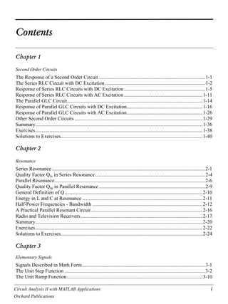
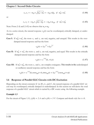
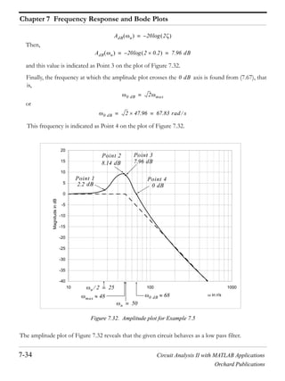
Other Second Order Circuits
and by substitution of given numerical values into (1.85) through (1.87), we get
or
(1.88)
(1.89)
(1.90)
Next, substitution of (1.89) and (1.90) into (1.88) yields
(1.91)
or
Division by yields
or
(1.92)
We use MATLAB to find the roots of the characteristic equation of (1.92).
syms s; y0=solve('s^2+2*10^3*s+2*10^6')
y0 =
[ -1000+1000*i]
[ -1000-1000*i]
that is,
1
2 10
5
------------------
1
4 10
4
------------------
1
5 10
4
------------------+ + v1 25 10
9– dv1
dt
--------
1
4 10
4
------------------vout–+
1
2 10
5
------------------vin=
0.05 10
3–
v1 25 10
9– dv1
dt
-------- 0.25 10
4–
vout–+ 0.5 10
5–
vin=
v1 5 10
4–
dvout
dt
-------------–=
dv1
dt
-------- 5 10
4– d
2
vout
dt
2
---------------–=
0.05 10
3–
5 10
4–
dvout
dt
-------------– 25 10
9–
5 10
4–
–
d
2
vout
dt
2
---------------
0.25 10
4–
vout–
+
0.5 10
5–
vin=
125– 10
13– d
2
vout
dt
2
--------------- 0.25 10
7–
dvout
dt
-------------– 0.25 10
4–
vout– 10
4–
vin=
125– 10
13–
d
2
vout
dt
2
---------------- 2 10
3
dvout
dt
------------- 2 10
6
vout+ + 1.6 10
5
– vin=
d
2
vout
dt
2
---------------- 2 10
3
dvout
dt
------------- 2 10
6
vout+ + 10
6
6280tcos–=

44. Chapter 1 Second Order Circuits
1-32 Circuit Analysis II with MATLAB Applications
Orchard Publications
We cannot classify the given circuit as series or parallel and therefore, we should not use the damping
ratio or . Instead, for the natural response we will use the general expression
(1.93)
where
Therefore, the natural response is oscillatory and has the form
(1.94)
Since the right side of (1.92) is a sinusoid, the forced response has the form
(1.95)
Of course, for the derivation of the forced response we could use phasor analysis but we must first
derive an expression for the impedance or admittance because the expressions we’ve used earlier are
valid for series and parallel circuits only.
The coefficients and will be found by substitution of (1.95) into (1.92) and then by equating
like terms. Using MATLAB we get:
syms t k3 k4; y0=k3*cos(6280*t)+k4*sin(6280*t); y1=diff(y0)
y1 =
-6280*k3*sin(6280*t)+6280*k4*cos(6280*t)
y2=diff(y0,2)
y2 =
-39438400*k3*cos(6280*t)-39438400*k4*sin(6280*t)
y=y2+2*10^3*y1+2*10^6*y0
y =
-37438400*k3*cos(6280*t)-37438400*k4*sin(6280*t)-
12560000*k3*sin(6280*t)+12560000*k4*cos(6280*t)
Equating like terms with (1.92) we get
(1.96)
Simultaneous solution of the equations of (1.96) is done with MATLAB.
s1 s2, – j 1000– j1000 1000 1– j1= = =
S P vn t
vn t Ae
s1t
= Be
s2t
+ e
t–
k1 tcos k2 tsin+=
s1 s2, – j 1000– j1000= =
vn t e
1000t–
k1 1000tcos k2 1000tsin+=
vf t k3 6280tcos k4 6280tsin+=
k3 k4
37438400 k3– 12560000 k4+ 6280tcos 10
6
– 6280tcos=
12560000 k3– 37438400 k4– 6280tsin 0=

45. 1-33 Circuit Analysis II with MATLAB Applications
Orchard Publications
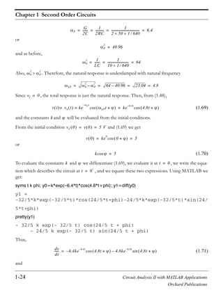
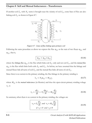
Other Second Order Circuits
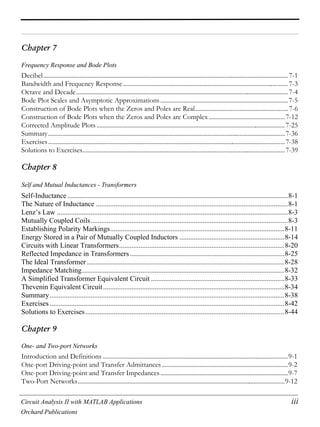
syms k3 k4; eq1= 37438400*k3+12560000*k4+10^6;...
eq2= 12560000*k3-37438400*k4+0; y=solve(eq1,eq2)
y =
k3: [1x1 sym]
k4: [1x1 sym]
y.k3
ans =
0.0240
y.k4
ans =
-0.0081
that is, and . Then, by substitution into (1.95)
(1.97)
The total response is
(1.98)
We will use the initial conditions to evaluate and . We observe that
and at relation (1.98) becomes
or and thus (1.98) simplifies to
(1.99)
To evaluate the constant , we make use of the initial condition . We observe that
and by KCL at node we have:
or
k3 0.024= k4 0.008–=
vf t 0.024 6280tcos 0.008– 6280tsin=
vout t vn t vf t+ e
1000t–
k1 1000tcos k2 1000tsin+
0.024 6280tcos 0.008– 6280tsin+
= =
vC1 vC2 0= = k1 k2 vC2 vout=
t 0=
vout 0 e
0
k1 0cos 0+ 0.024 0cos 0–+ 0= =
k1 0.024–=
vout t e
1000t–
0.024– 1000tcos k2 1000tsin+
0.024 6280tcos 0.008– 6280tsin+
=
k2 vC1 0 0=
vC1 v1= v1
v1 v2–
R3
--------------- C2
dvout
dt
-------------+ 0=
v1 0–
5 10
4
----------------- 10
8–
–=
dvout
dt
-------------

46. Chapter 1 Second Order Circuits
1-34 Circuit Analysis II with MATLAB Applications
Orchard Publications
or
and since , it follows that
(1.100)
The last step in finding the constant is to differentiate (1.99), evaluate it at , and equate it
with (1.100). This is done with MATLAB as follows:
y0=exp( 1000*t)*( 0.024*cos(1000*t)+k2*sin(1000*t))...
+0.024*cos(6280*t) 0.008*sin(6280*t);
y1=diff(y0)
y1 =
-1000*exp(-1000*t)*(-3/125*cos(1000*t)+k2*sin(1000*t))+exp(-
1000*t)*(24*sin(1000*t)+1000*k2*cos(1000*t))-3768/
25*sin(6280*t)-1256/25*cos(6280*t)
or
and
(1.101)
Simplifying and equating (1.100) with (1.101) we get
or
and by substitution into (1.99),
(1.102)
v1 5 10
4–
–=
dvout
dt
-------------
vC1 0 v1 0 0= =
dvout
dt
-------------
t 0=
0=
k2 t 0=
dvout
dt
------------- 1000e
1000t– 3–
125
--------- 1000t k2 1000tsin+cos–
e
1000t–
24 1000t 1000k2 1000tcos+sin
3768
25
------------ 6280tsin–
1256
25
------------ 6280tcos–
+
=
dvout
dt
-------------
t 0=
1000
3–
125
---------– 1000k2
1256
25
------------–+=
1000k2 26.24– 0=
k2 0.026=
vout t e
1000t–
0.024– 1000tcos 0.026 1000tsin+
0.024 6280tcos 0.008– 6280tsin+
=

47. 1-35 Circuit Analysis II with MATLAB Applications
Orchard Publications
Other Second Order Circuits
We use Excel to sketch . In Column A we enter several values of time and in Column B
. The plot is shown in Figure 1.20.
Figure 1.20. Plot for Example 1.7
vout t t
vout t
-0.03
-0.02
-0.01
0.00
0.01
0.02
0.03
0.000 0.002 0.004 0.006 0.008
Time (s)
Voltage(V)

48. Chapter 1 Second Order Circuits
1-36 Circuit Analysis II with MATLAB Applications
Orchard Publications
1.9 Summary
Circuits that contain energy storing devices can be described by integrodifferential equations and
upon differentiation can be simplified to differential equations with constant coefficients.
A second order circuit contains two energy storing devices. Thus, an RLC circuit is a second order
circuit.
The total response is the summation of the natural and forced responses.
If the differential equation describing a series RLC circuit that is excited by a constant (DC) volt-
age source is written in terms of the current, the forced response is zero and thus the total
response is just the natural response.
If the differential equation describing a parallel RLC circuit that is excited by a constant (DC) cur-
rent source is written in terms of the voltage, the forced response is zero and thus the total
response is just the natural response.
If a circuit is excited by a sinusoidal (AC) source, the forced response is never zero.
The natural response of a second order circuit may be overdamped, critically damped, or under-
damped depending on the values of the circuit constants.
For a series RLC circuit, the roots and are found from
or
where
If , the roots and are real, negative, and unequal. This results in the overdamped nat-
ural response and has the form
If , the roots and are real, negative, and equal. This results in the critically damped
natural response and has the form
s1 s2
s1 s2 S– S
2
0
2
– S– S if S
2
0
2
= =
s1 s2 S– 0
2
S
2
– S– nS
if 0
2
S
2
= =
S
R
2L
------= 0
1
LC
-----------= S S
2
0
2
–= nS 0
2
S
2
–=
S
2
0
2
s1 s2
in t k1e
s
1
t
k2e
s
2
t
+=
S
2
0
2
= s1 s2
in t e
St–
k1 k2t+=

49. 1-37 Circuit Analysis II with MATLAB Applications
Orchard Publications
Summary
If , the roots and are complex conjugates. This is known as the underdamped or
oscillatory natural response and has the form
For a parallel GLC circuit, the roots and are found from
or
where
If , the roots and are real, negative, and unequal. This results in the overdamped nat-
ural response and has the form
If , the roots and are real, negative, and equal. This results in the critically damped
natural response and has the form
If , the roots and are complex conjugates. This results in the underdamped or oscil-
latory natural response and has the form
If a second order circuit is neither series nor parallel, the natural response if found from
or
or
depending on the roots of the characteristic equation being real and unequal, real and equal, or
complex conjugates respectively.
0
2
S
2
s1 s2
in t e
S t–
k1 nS
cos t k2 nS
tsin+ k3e
St–
nS
cos t += =
s1 s2
s1 s2 P– P
2
0
2
– P– P if P
2
0
2
= =
s1 s2 P– 0
2
P
2
– P– nP if 0
2
P
2
= =
P
G
2C
-------= 0
1
LC
-----------= P P
2
0
2
–= nP 0
2
P
2
–=
P
2
0
2
s1 s2
vn t k1e
s
1
t
k2e
s
2
t
+=
P
2
0
2
= s1 s2
vn t e
Pt–
k1 k2t+=
0
2
P
2
s1 s2
vn t e
Pt–
k1 nPcos t k2 nPtsin+ k3e
Pt–
nPcos t += =
yn k1e
s1t
= k2e
s2t
+
yn k1 k2 t+ e
s1t
=
yn e
t–
k3 tcos k4 sin t+ e
t–
k5 t +cos==

50. Chapter 1 Second Order Circuits
1-38 Circuit Analysis II with MATLAB Applications
Orchard Publications
1.10 Exercises
1. For the circuit of Figure 1.21, it is known that and . Compute and sketch
and for .
Figure 1.21. Circuit for Exercise 1
2. For the circuit of Figure 1.22, it is known that and . Compute and sketch
and for .
Figure 1.22. Circuit for Exercise 2
3. In the circuit of Figure 1.23, the switch has been closed for a very long time and opens at
. Compute for .
Figure 1.23. Circuit for Exercise 3
vC 0 0= iL 0 0=
vC t iL t t 0
+
100u0 t V
10 0.2 H
8 mF
iL t
+
vC t
vC 0 0= iL 0 0=
vC t iL t t 0
+
100u0 t V
4 5 H
21.83 mF
iL t
+
vC t
S
t 0= vC t t 0
+
+
20 H100
100 V
400
vC t
1 120 F
S
t 0=

51. 1-39 Circuit Analysis II with MATLAB Applications
Orchard Publications
Exercises
4. In the circuit of Figure 1.24, the switch has been closed for a very long time and opens at .
Compute for .
Figure 1.24. Circuit for Exercise 4
5. In the circuit of Figure 1.25, the switch has been in position for closed for a very long time
and it is placed in position at . Find the value of that will cause the circuit to become
critically damped and then compute and for
Figure 1.25. Circuit for Exercise 5
6. In the circuit of Figure 1.26, the switch has been closed for a very long time and opens at .
Compute for .
Figure 1.26. Circuit for Exercise 6
S t 0=
vC t t 0
+
+
20 H100
400
vC t
1 120 F
S
t 0=
vS
vS 100 tcos u0 t V=
S A
B t 0= R
vC t iL t t 0
+ +
12 V
3
2
R
A
B
S
6
3 H
vC t
1 12 F
iL t
t 0=
S t 0=
vAB t t 0
+
12 V
4
2 H
1 4 F
BA
S t 0=
2

52. Chapter 1 Second Order Circuits
1-40 Circuit Analysis II with MATLAB Applications
Orchard Publications
1.11 Solutions to Exercises
Dear Reader:
The remaining pages on this chapter contain the solutions to the exercises.
You must, for your benefit, make an honest effort to find the solutions to the exercises without first
looking at the solutions that follow. It is recommended that first you go through and work out those
you feel that you know. For the exercises that you are uncertain, review this chapter and try again.
Refer to the solutions as a last resort and rework those exercises at a later date.
You should follow this practice with the rest of the exercises of this book.

53. 1-41 Circuit Analysis II with MATLAB Applications
Orchard Publications
Solutions to Exercises
1.
and since , the above becomes
From the characteristic equation
we get (critical damping) and
The total solution is
(1)
With the first initial condition the above expression becomes or
and by substitution into (1) we get
(2)
To evaluate we make use of the second initial condition and since , and
, we differentiate (2) using the following MATLAB code:
+
100u0 t V
10 0.2 H
8 mF
iL t
+
vC t
i
Ri L
di
dt
----- vC+ + 100= t 0
i iC C
dvC
dt
--------= =
RC
dvC
dt
-------- LC
d
2
vC
dt
2
---------- vC+ + 100=
d
2
vC
dt
2
----------
R
L
---
dvC
dt
-------- 1
LC
-------vC+ +
100
LC
---------=
d
2
vC
dt
2
----------
10
0.2
-------
dvC
dt
-------- 1
0.2 8 10
3–
--------------------------------- vC+ + 100
0.2 8 10
3–
---------------------------------=
d
2
vC
dt
2
---------- 50
dvC
dt
-------- 625 vC+ + 62500=
s
2
50s 625+ + 0=
s1 s2 25–= = S R 2L 25= =
vC t vCf vCn+ 100 e
S t–
k1 k2t++ 100 e
25 t–
k1 k2t++= = =
vC 0 0= 0 100 e
0
k1 0++=
k1 100–=
vC t 100 e
25 t–
k2t 100–+=
k2 iL 0 0= iL iC=
i iC C dvC dt= =

54. Chapter 1 Second Order Circuits
1-42 Circuit Analysis II with MATLAB Applications
Orchard Publications
syms t k2
v0=100+exp( 25*t)*(k2*t 100); v1=diff(v0)
v1 =
-25*exp(-25*t)*(k2*t-100)+exp(-25*t)*k2
Thus,
and
(3)
Also, and at
(4)
From (3) and (4) or and by substitution into (2)
(5)
We find by differentiating (5) and multiplication by . Using MATLAB we get:
syms t
C=8*10^( 3);
i0=C*(100-exp( 25*t)*(100+2500*t)); iL=diff(i0)
iL =
1/5*exp(-25*t)*(100+2500*t)-20*exp(-25*t)
Thus,
The plots for and are shown on the next page.
dvC
dt
-------- k2 e
25t–
25e
25t–
k2 t 100––=
dvC
dt
--------
t 0=
k2 2500+=
dvC
dt
--------
iC
C
----
iL
C
----= = t 0=
dvC
dt
--------
t 0=
iL 0
C
--------------- 0= =
k2 2500+ 0= k2 2500–=
vC t 100 e
25t–
– 2500t 100+=
iL t iC t= C
iL t iC t 0.2e
25t–
100 2500t+ 20e
25t–
–= =
vC t iL t

55. 1-43 Circuit Analysis II with MATLAB Applications
Orchard Publications
Solutions to Exercises
2.
The general form of the differential equation that describes this circuit is same as in Exercise 1,
that is,
From the characteristic equation and the MATLAB code below
t vC(t) iL(t)
0.000 0 0
0.005 0.7191 2.206
0.010 2.6499 3.894
0.015 5.4977 5.155
0.020 9.0204 6.065
0.025 13.02 6.691
0.030 17.336 7.085
0.035 21.838 7.295
0.040 26.424 7.358
0.045 31.011 7.305
0.050 35.536 7.163
0.055 39.951 6.953
0.060 44.217 6.694
0.065 48.311 6.4
0.070 52.212 6.082
0.075 55.91 5.751
0.080 59.399 5.413
0.085 62.677 5.076
0.090 65.745 4.743
0.095 68.608 4.418
0.100 71.27 4.104
0.105 73.741 3.803
0.110 76.027 3.516
0.115 78.139 3.244
vC(t)
0
20
40
60
80
100
0.0 0.1 0.2 0.3 0.4 0.5
Time
Volts
iL(t)
0
2
4
6
8
0.0 0.1 0.2 0.3 0.4 0.5
Time
Amps
+
100u0 t V
4 5 H
21.83 mF
iL t
+
vC t
d
2
vC
dt
2
----------
R
L
---
dvC
dt
--------
1
LC
-------vC+ +
100
LC
---------= t 0
d
2
vC
dt
2
---------- 0.8
dvC
dt
-------- 9.16vC+ + 916=
s
2
0.8s 9.16+ + 0=

56. Chapter 1 Second Order Circuits
1-44 Circuit Analysis II with MATLAB Applications
Orchard Publications
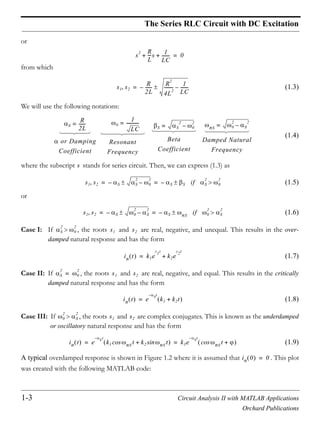
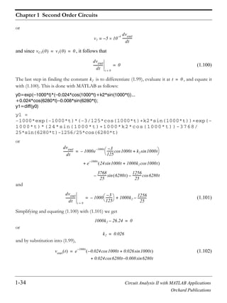
s=[1 0.8 9.16]; roots(s)
ans =
-0.4000 + 3.0000i
-0.4000 - 3.0000i
we find that and . Therefore, the total solution is
where
and
Thus,
(1)
and with the initial condition we get or
(2)
To evaluate and we differentiate (1) with MATLAB and evaluate it at .
syms t k phi; v0=100+k*exp( 0.4*t)*cos(3*t+phi); v1=diff(v0)
v1 =
-2/5*k*exp(-2/5*t)*cos(3*t+phi)-3*k*exp(-2/5*t)*sin(3*t+phi)
Thus,
and with (2)
(3)
Also, and at
(4)
s1 0.4– j3+= s2 0.4– j3–=
vC t vCf vCn+ 100 ke
St–
nS
t +cos+= =
S R 2L 0.4= =
nS 0
2
S
2
– 1 LC R
2
4L
2
– 9.16 0.16– 3= = = =
vC t 100 ke
0.4t–
3t +cos+=
vC 0 0= 0 100 k 0 +cos+=
kcos 100–=
k t 0=
dvC
dt
-------- 0.4k– e
0.4t–
3t +cos 3ke
0.4t–
3 t +sin–=
dvC
dt
--------
t 0=
0.4k– cos 3ksin–=
dvC
dt
--------
t 0=
40 3ksin–=
dvC
dt
--------
iC
C
----
iL
C
----= = t 0=
dvC
dt
--------
t 0=
iL 0
C
--------------- 0= =

57. 1-45 Circuit Analysis II with MATLAB Applications
Orchard Publications
Solutions to Exercises
From (3) and (4)
(5)
and from (2) and (5)
The value of can be found from either (2) or (5). From (2)
and by substitution into (1)
(6)
Since , we use MATLAB to differentiate (6).
syms t; vC=100 100.8*exp( 0.4*t)*cos(3*t 0.1326); C=0.02183; iL=C*diff(vC)
iL =
137529/156250*exp(-2/5*t)*cos(3*t-663/5000)+412587/62500*exp(-
2/5*t)*sin(3*t-663/5000)
137529/156250, 412587/62500
ans =
0.8802
ans =
6.6014
The plots for and are shown on the next page.
3ksin 40=
3ksin
kcos
-----------------
40
100–
------------=
3tan 0.4–=
0.4– 31–tan 0.1326 rad– 7.6–= = =
k
k 0.1236–cos 100–=
k
100–
0.1236–cos
--------------------------------- 100.8–= =
vC t 100 100.8– e
0.4t–
3t 7.6–cos=
iL t iC t C dvC dt= =
iL t 0.88e
0.4t–
3t 7.6– 6.6e
0.4t–
3t 7.6–sin+cos=
vC t iL t

58. Chapter 1 Second Order Circuits
1-46 Circuit Analysis II with MATLAB Applications
Orchard Publications
3.
At the circuit is as shown below.
At this time the inductor behaves as a short and the capacitor as an open. Then,
and this establishes the first initial condition as . Also,
and this establishes the first initial condition as .
For the circuit is as shown below.
t vC(t) iL(t)
0.000 -0.014 -0.002
0.010 0.0313 0.198
0.020 0.1677 0.395
0.030 0.394 0.591
0.040 0.7094 0.784
0.050 1.1129 0.975
0.060 1.6034 1.164
0.070 2.1798 1.35
0.080 2.8407 1.534
0.090 3.5851 1.714
0.100 4.4115 1.892
0.110 5.3185 2.066
0.120 6.3046 2.238
0.130 7.3684 2.405
0.140 8.5082 2.57
0.150 9.7224 2.73
0.160 11.009 2.887
vC(t)
-50
50
150
0 3 6 9 12
iL(t)
-10
10
0 3 6 9 12
t 0=
+
+
20 H100
100 V
400
vC 0
1 120 F
iL 0
iL 0 100 100 400+ I0 0.2 A= = =
I0 0.2 A=
vC 0 v400 400 iL 0 400 0.2 V0 80 V= = = = =
V0 80 V=
t 0

59. 1-47 Circuit Analysis II with MATLAB Applications
Orchard Publications
Solutions to Exercises
The general form of the differential equation that describes this circuit is same as in Exercise 1,
that is,
From the characteristic equation we find that and and the total
response for the capacitor voltage is
(1)
Using the initial condition we get
or
(2)
Differentiation of (1) and evaluation at yields
(3)
Also, and at
(4)
Equating (3) and (4) we get
(5)
and simultaneous solution of (2) and (5) yields and .
+
+
20 H100
100 V
vC t
1 120 F
d
2
vC
dt
2
----------
R
L
---
dvC
dt
--------
1
LC
-------vC+ +
100
LC
---------= t 0
d
2
vC
dt
2
---------- 5
dvC
dt
-------- 6vC+ + 600=
s
2
5s 6+ + 0= s1 2–= s2 3–=
vC t vCf vCn+ 100 k1e
s1t
k2e
s2t
+ + 100 k1e
2t–
k2e
3t–
+ += = =
V0 80 V=
vC 0 V0 80 V 100 k1e
0
k2e
0
+ += ==
k1 k2+ 20–=
t 0=
dvC
dt
--------
t 0=
2k1– 3k2–=
dvC
dt
--------
iC
C
----
iL
C
----= = t 0=
dvC
dt
--------
t 0=
iL 0
C
--------------- 0.2
1 120
---------------- 24= = =
2k1– 3k2– 24=
k1 36–= k2 16=

60. Chapter 1 Second Order Circuits
1-48 Circuit Analysis II with MATLAB Applications
Orchard Publications
By substitution into (1) we find the total solution as
4.
This is the same circuit as in Exercise 3 where the DC voltage source has been replaced by an AC
source that is being applied at . No initial conditions were given so we will assume that
and . Also, the circuit constants are the same and thus the natural
response has the form .
We will find the forced (steady-state) response using phasor circuit analysis where ,
, , and . The phasor circuit is shown below.
Using the voltage division expression we get
and in the -domain . Therefore, the total response is
(1)
Using the initial condition and (1) we get
vC t vCf vCn+ 100 36– e
2t–
16e
3t–
+= =
+
+
20 H100
400
vC t
1 120 F
S
t 0=
vS
vS 100 tcos u0 t V=
t 0
+
=
iL 0 0= vC 0 0=
vCn k1e
2t–
k2e
3t–
+=
1=
j L j20= j– C j120–= 100 t 100 0cos
+
+
j20100
VS
VS 100 0 V=
VCj– 120
VC
j120–
100 j20 j120–+
----------------------------------------100 0
j120–
100 j100+
--------------------------100 0
120 90 100 0–
100 2 45
---------------------------------------------------- 60 2 135–= = ==
t vCf 60 2 t 135–cos=
vC t 60 2 t 135–cos k1e
2t–
k2e
3t–
+ +=
vC 0 0=

61. 1-49 Circuit Analysis II with MATLAB Applications
Orchard Publications
Solutions to Exercises
and since the above expression reduces to
(2)
Differentiating (1) we get
and
(3)
Also, and at
(4)
Equating (3) and (4) we get
(5)
Simultaneous solution of (2) and (5) yields and . Then, by substitution into (1)
5.
We must first find the value of before we can establish initial conditions for and
. The condition for critical damping is where
vC 0 0 60 2 135–cos k1 k2+ += =
135–cos 2– 2=
k1 k2+ 60=
dvC
dt
-------- 60 2 t 45+sin 2k– 1e
2t–
3k2– e
3t–
+=
dvC
dt
--------
t 0=
60 2 45sin 2k– 1 3k2–=
dvC
dt
--------
t 0=
60 2k– 1 3k2–=
dvC
dt
--------
iC
C
----
iL
C
----= = t 0=
dvC
dt
--------
t 0=
iL 0
C
--------------- 0= =
2k1 3k2+ 60=
k1 120= k2 60–=
vC t 60 2 t 135–cos 120e
2t–
60– e
3t–
+=
+ +
12 V
3
2
R
A
B
S
6
3 H
vC t
1 12 F
iL t
t 0=
R iL 0 0=
vC 0 0= P
2
0
2
– 0= P G 2C 1 2R'C= =

62. Chapter 1 Second Order Circuits
1-50 Circuit Analysis II with MATLAB Applications
Orchard Publications
and . Then, where . Therefore,
, or , or , or and thus .
At the circuit is as shown below.
From the circuit above
and
At the circuit is as shown below.
Since the circuit is critically damped, the solution has the form
where and thus
(1)
0
2
1 LC= P
2 1
2R' 1 12
---------------------------
2
0
2
= = 1
3 1 12
----------------------= R' R 2+=
12
2 R 2+
---------------------
2
4=
6
R 2+
-------------
2
4= R 2+
2
36 4 9= = R 2+ 3= R 1=
t 0=
+ +
12 V
3 1
6
vC 0
iL 0
v6+
vC 0 v6
6
3 1 6+ +
--------------------- 12 7.2 V= = =
iL 0
v6
6
---------
7.2
6
------- 1.2 A= = =
t 0
+
=
+
6
3 H
vC t
1 12 F
iL t
1
2
iC t
iR t
vC t e
P t–
k1 k2t+=
P
1
2 1 2+ 1 12
--------------------------------------- 2= =
vC t e
2 t–
k1 k2t+=

63. 1-51 Circuit Analysis II with MATLAB Applications
Orchard Publications
Solutions to Exercises
With the initial condition relation (1) becomes or
and (1) simplifies to
(2)
Differentiating (2) we get
and
(3)
Also, and at
(4)
because at the capacitor is an open circuit.
Equating (3) and (4) we get or and by substitution into (2)
We find from or where
and . Then,
6.
At the circuit is as shown below where , , and thus
the initial conditions have been established.
vC 0 7.2 V= 7.2 e
0
k1 0+= k1 7.2 V=
vC t e
2 t–
7.2 k2t+=
dvC
dt
-------- k2 e
2– t
2e
2 t–
7.2 k2t+–=
dvC
dt
--------
t 0=
k2 2 7.2 0+– k2 14.4–= =
dvC
dt
--------
iC
C
----= t 0=
dvC
dt
--------
t 0=
iC 0
C
------------
0
C
---- 0= = =
t 0=
k2 14.4– 0= k2 14.4=
vC t e
2 t–
7.2 14.4t+ 7.2e
2t–
2t 1+= =
iL t iR t iC t iL t+ + 0= iL t iC t iR t––= iC t C dvC dt=
iR t vR t 1 2+ vC t 3= =
iL t
1
12
------ 14.4e
2t–
2t 1+ 14.4e
2t–
+––
7.2
3
-------e
2t–
2t 1+– 2.4e
2t–
t 1+–= =
t 0= iL 0 12 2 6 A= = vC 0 12 V=
+
12 V
4
2 H
1 4 F
BA
2
+
vC 0
iL 0

64. Chapter 1 Second Order Circuits
1-52 Circuit Analysis II with MATLAB Applications
Orchard Publications
For the circuit is as shown below.
For this circuit
and with the above relation can be written as
The characteristic equation of the last expression above yields and and thus
(1)
With the initial condition and (1) we get
(2)
Differentiating (1) we get
and
(3)
Also, and at
t 0
4
2 H 1 4 F
BA
2
+
vC t
iL t
R1 R2
L
C
R1 R2+ iL vC L
diL
dt
-------+ + 0=
iL iC C dvC dt= =
R1 R2+ C
dvC
dt
-------- LC
d
2
vC
dt
2
---------- vC+ + 0=
d
2
vC
dt
2
----------
R1 R2+
L
----------------------
dvC
dt
--------
1
LC
-------vC+ + 0=
d
2
vC
dt
2
---------- 3
dvC
dt
-------- 2vC+ + 0=
s1 1–= s2 2–=
vC t k1e
t–
k2 e
2t–
+=
vC 0 12 V=
k1 k2+ 12=
dvC
dt
-------- k– 1e
t–
2k2– e
2t–
=
dvC
dt
--------
t 0=
k– 1 2k2–=
dvC
dt
--------
iC
C
----
iL
C
----= = t 0=

65. 1-53 Circuit Analysis II with MATLAB Applications
Orchard Publications
Solutions to Exercises
(4)
From (3) and (4)
(5)
and from (2) and (5) and . By substitution into (1) we get
Then,
dvC
dt
--------
t 0=
iL 0
C
------------
6
1 4
---------- 24= = =
k– 1 2k2– 24=
k1 48= k2 36–=
vC t 48e
t–
36– e
2t–
=
vAB vL t vC t– L
diL
dt
------- vC t– LC
d
2
iC
dt
2
---------- vC t–= = =
0.5
d
2
dt
2
------- 48e
t–
36– e
2t–
48e
t–
36– e
2t–
–=
0.5 48e
t–
144– e
2t–
48e
t–
36– e
2t–
–=
24– e
t–
108– e
2t–
24 e
t–
4.5e
2t–
+–==

66. Chapter 1 Second Order Circuits
1-54 Circuit Analysis II with MATLAB Applications
Orchard Publications
NOTES

67. Circuit Analysis II with MATLAB Applications 2-1
Orchard Publications
Chapter 2
Resonance
his chapter defines series and parallel resonance. The quality factor is then defined in terms
of the series and parallel resonant frequencies. The half-power frequencies and bandwidth are
also defined in terms of the resonant frequency.
2.1 Series Resonance
Consider phasor series circuit of Figure 2.1.
Figure 2.1. Series RLC phasor circuit
The impedance is
(2.1)
or
(2.2)
Therefore, the magnitude and phase angle of the impedance are:
(2.3)
and
(2.4)
The components of are shown on the plot of Figure 2.2.
T
Q
RLC
VS
I
R
1 j C
j L
Z
Impedance Z
Phasor Voltage
Phasor Current
---------------------------------------
VS
I
------ R j L
1
j C
----------+ + R j L
1
C
--------–+= = = = =
Z R
2
L 1 C–
2
+ L 1 C– R
1–
tan=
Z R
2
L 1 C–
2
+=
Z L 1 C– R
1–
tan=
Z

68. Chapter 2 Resonance
2-2 Circuit Analysis II with MATLAB Applications
Orchard Publications
Figure 2.2. The components of in a series RLC circuit
The frequency at which the capacitive reactance and the inductive reactance
are equal is called the resonant frequency. The resonant frequency is denoted as or and these
can be expressed in terms of the inductance and capacitance by equating the reactances, that is,
(2.5)
and
(2.6)
We observe that at resonance where denotes the impedance value at resonance, and
. In our subsequent discussion the subscript zero will be used to indicate that the circuit vari-
ables are at resonance.
Example 2.1
For the circuit shown in Figure 2.3, compute , , , , , and . Then, draw a phasor
diagram showing , , and .
Series Resonance Curves
Radian Frequency
MagnitudeofImpedance
0
1 / C
|Z|
R
L
L 1 / C
0
Z
XC 1 C= XL L=
0 f0
L C
0L 1
0C
----------=
0
2 1
LC
-------=
0
1
LC
-----------=
f0
1
2 LC
------------------=
Z0 R= Z0
Z 0=
I0 0 C VR0 VL0 VC0
VR0 VL0 VC0

69. Circuit Analysis II with MATLAB Applications 2-3
Orchard Publications
Series Resonance
Figure 2.3. Circuit for Example 2.1
Solution:
At resonance,
and thus
Then,
Since
it follows that
Therefore,
or
Now,
and
The phasor diagram showing , , and is shown in Figure 2.4.
VS
I
L=0.2 mH
C
j– XC120 0 V
R 1.2= jXL j10=
jXL jXC–=
Z0 R 1.2= =
I0
120 V
1.2
-------------- 100 A= =
XL0 0L 10= =
0
10
L
------
10
0.2 10
3–
------------------------ 50000 rad s= = =
XC0 XL0 10
1
0C
----------= = =
C
1
10 50000
--------------------------- 2 F= =
VR0 RI0 1.2 100 120 V= = =
VL0 0LI0 50000 0.2 10
3–
100 1000= = =
VC0
1
0C
----------I0
1
50000 2 10
6–
----------------------------------------- 100 1000 V= = =
VR0 VL0 VC0

70. Chapter 2 Resonance
2-4 Circuit Analysis II with MATLAB Applications
Orchard Publications
Figure 2.4. Phasor diagram for Example 2.1
Figure 2.4 reveals that and these voltages are much higher than the applied
voltage of . This illustrates the useful property of resonant circuits to develop high voltages
across capacitors and inductors.
2.2 Quality Factor Q0s in Series Resonance
The quality factor *
is an important parameter in resonant circuits. Its definition is derived from the
following relations:
At resonance,
and
Then
(2.7)
and
(2.8)
At series resonance the left sides of (2.7) and (2.8) are equal and therefore,
* We denote the quality factor for series resonant circuits as , and the quality factor for parallel resonant cir-
cuits as .
VR0 = 120 V
|VL0| = 1000 V
|VC0| = 1000 V
VL0 VC0 1000 V= =
120 V
Q0S
Q0P
0L 1
0C
----------=
I0
VS
R
---------=
VL0 0LI0 0L
VS
R
--------- 0L
R
--------- VS= = =
VC0
1
0C
----------I0
1
0C
----------
VS
R
---------
1
0RC
-------------- VS= = =
0L
R
---------
1
0RC
--------------=

71. Circuit Analysis II with MATLAB Applications 2-5
Orchard Publications
Quality Factor Q0s in Series Resonance
Then, by definition
(2.9)
In a practical circuit, the resistance in the definition of above, represents the resistance of the
inductor and thus the quality factor is a measure of the energy storage property of the inductance
in relation to the energy dissipation property of the resistance of that inductance.
In terms of , the magnitude of the voltages across the inductor and capacitor are
(2.10)
and therefore, we say that there is a “resonant” rise in the voltage across the reactive devices and it is
equal to the times the applied voltage. Thus in Example 2.1,
The quality factor is also a measure of frequency selectivity. Thus, we say that a circuit with a high
has a high selectivity, whereas a low circuit has low selectivity. The high frequency selectivity is
more desirable in parallel circuits as we will see in the next section.
Figure 2.5 shows the relative response versus for , and where we observe that
highest provides the best frequency selectivity, i.e., higher rejection of signal components outside
the bandwidth which is the difference in the frequencies.
Figure 2.5. Selectivity curves with , and
Q0S
0L
R
---------
1
0RC
--------------= =
Quality Factor at Series Resonance
R Q0S
Q0S
L R
Q0S
VL0 VC0 Q0S VS= =
Q0S
Q0S
VL0
VS
------------
VC0
VS
------------
1000
120
------------
25
3
------= = = =
Q
Q Q
Q 25 50= 100
Q
BW 2 1–= 3 dB
Selectivity Curves for Different Qs
0.0
0.2
0.4
0.6
0.8
1.0
1.2
r/s
RelativeResponse(gain)
1 0 2
Q=25
Q=50
Q=100
Q 25 50= 100

72. Chapter 2 Resonance
2-6 Circuit Analysis II with MATLAB Applications
Orchard Publications
We will see later that
(2.11)
We also observe from (2.9) that selectivity depends on and this dependence is shown on the plot
of Figure 2.6.
Figure 2.6. Selectivity curves with different values of R
If we keep one reactive device, say , constant while varying , the relative response “shifts” as
shown in Figure 2.7, but the general shape does not change.
Figure 2.7. Relative response with constant L and variable C
2.3 Parallel Resonance
Parallel resonance (antiresonance) applies to parallel circuits such as that shown in Figure 2.8.
Q 0
2 1–
------------------ Resonant Frequency
Bandwidth
-------------------------------------------------------= =
R
High and Low Q Curves
Dependence on R
RelativeResponse
R
2R
L C
Resonance at Constant L and Variable C
RelativeResponse
C
0.5C

73. Circuit Analysis II with MATLAB Applications 2-7
Orchard Publications
Parallel Resonance
Figure 2.8. Parallel GLC circuit for defining parallel resonance
The admittance of this circuit is given by
or
(2.12)
Therefore, the magnitude and phase angle of the admittance are:
(2.13)
and
(2.14)
The frequency at which the inductive susceptance and the capacitive susceptance
are equal is, again, called the resonant frequency and it is also denoted as We can find
in terms of and as before.
Since
then,
and
(2.15)
as before. The components of are shown on the plot of Figure 2.2.
V G L
C
+
ICIG IL
IS
Y
Admit cetan Y Phasor Current
Phasor Voltage
-------------------------------------
IS
V
---- G j C 1
j L
---------+ + G j C 1
L
-------–+= = = = =
Y G
2
C 1 L–
2
+ C 1 L– G1–
tan=
Y
Y G
2
C 1 L–
2
+=
Y
C 1 L–
G
---------------------------------
1–
tan=
BL 1 L=
BC C= 0
0 L C
0C 1
0L
---------–
0C
1
0L
---------=
0
1
LC
-----------=
Y

74. Chapter 2 Resonance
2-8 Circuit Analysis II with MATLAB Applications
Orchard Publications
Figure 2.9. The components of in a parallel RLC circuit
We observe that at this parallel resonant frequency,
(2.16)
and
(2.17)
Example 2.2
For the circuit of Figure 2.10, . Compute , , and .
Figure 2.10. Circuit for Example 2.2
Solution:
The capacitive and inductive susceptances are
and
and since , the given circuit operates at parallel resonance with . Then,
Parallel Resonance Curves
Radian Frequency
MagnitudeofAdmittance
0
1 / L
|Y|
G
C
C 1/ L
0
Y
Y0 G=
Y 0=
iS t 10 5000t mAcos= iG t iL t iC t
G L C
+
10 mHiS t
iG t
iL t iC t
v t
0.01
1– 4 F
BC C 5000 4 10
6–
0.02
1–
= = =
BL
1
L
-------
1
5000 10 10
3–
----------------------------------------- 0.02
1–
= = =
BL BC= 0 5000 rad s=

75. Circuit Analysis II with MATLAB Applications 2-9
Orchard Publications
Quality Factor Q0p in Parallel Resonance
and
Next, to compute and , we must first find . For this example,
In phasor form,
Now,
and in the -domain,
or
Similarly,
and in the -domain,
or
We observe that as expected.
2.4 Quality Factor Q0p in Parallel Resonance
At parallel resonance,
and
Then,
(2.18)
Also,
Y0 G 0.01
1–
= =
iG t iS t 10 5000t mAcos= =
iL t iC t v0 t
v0 t
iG t
G
------------ 10 5000t mAcos
0.01
1–
--------------------------------------- 1000 5000t mVcos 5000t Vcos= = = =
v0 t 5000t Vcos= V0 1 0=
IL0 jBL– V0 1 90– 0.02 1 0 0.02 90– A= = =
t
IL0 0.02 90– A= iL0 t 0.02 5000t 90– Acos=
iL0 t 20 5000t mAsin=
IC0 jBCV0 1 90 0.02 1 0 0.02 90 A= = =
t
IC0 0.02 90 A= iC0 t 0.02 5000t 90+ Acos=
iC0 t 20– 5000t mAsin=
iL0 t iC0 t+ 0=
0C
1
0L
---------=
V0
IS
G
-------=
IC0 0CV0 0C
IS
G
------- 0C
G
---------- IS= = =

76. Chapter 2 Resonance
2-10 Circuit Analysis II with MATLAB Applications
Orchard Publications
(2.19)
At parallel resonance the left sides of (2.18) and (2.19) are equal and therefore,
Now, by definition
(2.20)
The above expressions indicate that at parallel resonance, it is possible to develop high currents
through the capacitors and inductors. This was found to be true in Example 2.2.
2.5 General Definition of Q
The general (and best) definition of is
(2.21)
Essentially, the resonant frequency is the frequency at which the inductor gives up energy just as fast
as the capacitor requires it during one quarter cycle, and absorbs energy just as fast as it is released by
the capacitor during the next quarter cycle. This can be seen from Figure 2.11 where at the instant of
maximum current the energy is all stored in the inductance, and at the instant of zero current all the
energy is stored in the capacitor.
Figure 2.11. Waveforms for and at resonance
IL0
1
0L
---------V0
1
0L
---------
VS
G
---------
1
0GL
-------------- IS= = =
0C
G
---------- 1
0GL
--------------=
Q0P
0C
G
----------
1
0GL
--------------= =
Quality Factor at Parallel Resonance
Q
Q 2
Maximum Energy Stored
Energy Dissipated per Cycle
------------------------------------------------------------------------------=
WL & WC in Series RLC Circuit
Energy(J)
W L W C
v C i L
WL WC

77. Circuit Analysis II with MATLAB Applications 2-11
Orchard Publications
Energy in L and C at Resonance
2.6 Energy in L and C at Resonance
For a series circuit we let
Then,
Also,
(2.22)
and
(2.23)
Therefore, by (2.22) and (2.23), the total energy at any instant is
(2.24)
and this expression is true for any series circuit, that is, the circuit need not be at resonance. How-
ever, at resonance,
or
By substitution into (2.24),
(2.25)
and (2.25) shows that the total energy is dependent only on the circuit constants , and res-
onant frequency, but it is independent of time.
Next, using the general definition of we get:
RLC
i Ip tcos C
dvC
dt
---------= =
vC
Ip
C
-------- tsin=
WL
1
2
---Li
2 1
2
---LIp
2
t
2
cos= =
WC
1
2
---Cv
2 1
2
---
Ip
2
2
C
---------- t
2
sin= =
WT
WT WL WC+
1
2
---Ip
2
L t
2
cos
1
2
C
---------- t
2
sin+= =
0L 1
0C
----------=
L 1
0
2
C
----------=
WT
1
2
---Ip
2
L 0t
2
cos L 0t
2
sin+
1
2
---Ip
2
L
1
2
---Ip
2 1
0
2
C
----------= = =
WT L C
Q
Q0S 2
Maximum Energy Stored
Energy Dissipated per Cycle
------------------------------------------------------------------------------ 2
1 2 Ip
2
L
1 2 Ip
2
R f0
-------------------------------- 2
f0L
R
-------= = =

78. Chapter 2 Resonance
2-12 Circuit Analysis II with MATLAB Applications
Orchard Publications
or
(2.26)
and we observe that (2.26) is the same as (2.9). Similarly,
or
(2.27)
and this is also the same as (2.9).
Following the same procedure for a simple (or ) parallel circuit we can show that:
(2.28)
and this is the same as (2.20).
2.7 Half-Power Frequencies - Bandwidth
Parallel resonance is by far more important and practical than series resonance and therefore, the
remaining discussion will be on parallel (or ) circuits.
The plot of Figure 2.12 shows the magnitude of the voltage response versus radian frequency for a
typical parallel circuit.
Figure 2.12. Relative voltage vs.radian frequency in a parallel circuit
Q0S
0L
R
---------=
Q0S 2
Maximum Energy Stored
Energy Dissipated per Cycle
------------------------------------------------------------------------------ 2
1 2 Ip
2
1 0
2
C
1 2 Ip
2
R f0
------------------------------------------- 2
f0
0
2
RC
--------------= = =
Q0S
0
0
2
RC
---------------- 1
0RC
--------------= =
GLC RLC
Q0P
0C
G
----------
1
0LG
--------------= =
GLC RLC
RLC
Bandwidth in Parallel RLC Circuit
RelativeVoltage
1 20
0.707Vp
Vp
RLC

79. Circuit Analysis II with MATLAB Applications 2-13
Orchard Publications
Half-Power Frequencies - Bandwidth
By definition, the half-power frequencies and in Figure 2.12 are the frequencies at which the
magnitude of the input admittance of a parallel resonant circuit, is greater than the magnitude at res-
onance by a factor of , or equivalently, the frequencies at which the magnitude of the input
impedance of a parallel resonant circuit, is less than the magnitude at resonance by a factor of as
shown above. We observe also, that and are not exactly equidistant from . However, it is
convenient to assume that they are equidistant, and unless otherwise stated, this assumption will be
followed in the subsequent discussion.
We call the lower half-power point, and the upper half-power point. The difference is
the half-power bandwidth , that is,
(2.29)
The names half-power frequencies and half-power bandwidth arise from the fact that the power at
these frequencies drop to since .
The bandwidth can also be expressed in terms of the quality factor as follows:
Consider the admittance
Multiplying the term by , we get
Recalling that for parallel resonance
by substitution we get
(2.30)
and if , then
1 2
2
2
1 2 0
1 2 2 1–
BW
Bandwidth BW 2 1–= =
0.5 2 2
2
0.5=
BW Q
Y G j C
1
L
-------–+=
j G
0
0G
----------
Y G jG 0C
0G
-------------- 0
0LG
------------------–+=
Q0P
0C
G
---------- 1
0LG
--------------= =
Y G 1 jQ0P
0
------ 0
------–+=
0=
Y G=

80. Chapter 2 Resonance
2-14 Circuit Analysis II with MATLAB Applications
Orchard Publications
Next, we want to find the bandwidth in terms of the quality factor . At the half-power
points, the magnitude of the admittance is and, if we use the half-power points as refer-
ence, then to obtain the admittance value of
we must set
for .
We must also set
for .
Recalling that and solving the above expressions for and , we get
(2.31)
and
(2.32)
Subtraction of (2.32) from (2.31) yields
(2.33)
or
(2.34)
As mentioned earlier, and are not equidistant from In fact, the resonant frequency is
the geometric mean* of and , that is,
(2.35)
* The geometric mean of n positive numbers , ,..., is the nth root of the product.
2 1– Q0P
2 2 Yp
|Ymax 2G=
Q0P
2
0
------ 0
2
------– 1=
2=
Q0P
1
0
------ 0
1
------– 1–=
1=
1 j1 2= 1 2
2 1
1
2Q0P
-------------
2
+
1
2Q0P
-------------+=
1 1
1
2Q0P
-------------
2
+ 1
2Q0P
-------------–=
BW 2 1– 0
Q0P
---------= =
BW f2 f1–
f0
Q0P
---------= =
1 2 0 0
1 2
a1 a2 an a1 a2 an
0 1 2=

81. Circuit Analysis II with MATLAB Applications 2-15
Orchard Publications
Half-Power Frequencies - Bandwidth
This can be shown by multiplication of the two expressions in (2.31) and (2.32) and substitution into
(2.33).
Example 2.3
For the network of Figure 2.13, find:
a.
b.
c.
d.
e.
Figure 2.13. Network for Example 2.3
Solution:
a.
or
b.
c.
d.
e.
0
Q0P
BW
1
2
Y G L C
1 mH0.001
1–
0.4 F
0
2 1
LC
-------
1
1 10
3–
0.4 10
6–
-------------------------------------------------- 25 10
8
= = =
0 50000 r s=
Q0P
0C
G
---------- 5 10
4
0.4 10
6–
10
3–
------------------------------------------------ 20== =
BW 0
Q0P
---------
50000
20
--------------- 2500= rad s= = =
1 0
BW
2
---------– 50000 1250– 48750 rad s= = =
2 0
BW
2
---------+ 50000 1250+ 51250 rad s= = =

82. Chapter 2 Resonance
2-16 Circuit Analysis II with MATLAB Applications
Orchard Publications
2.8 A Practical Parallel Resonant Circuit
In our previous discussion, we assumed that the inductors are ideal, but a real inductor has some
resistance. The circuit shown in Figure 2.14 is a practical parallel resonant circuit.
Figure 2.14. A practical parallel resonant circuit
To derive an expression for its resonant frequency, we proceed as follows:
The resonant frequency is independent of the conductance and, for simplicity, it is omitted from
the network of Figure 2.14. We will therefore, find an expression for the network of Figure 2.15.
Figure 2.15. Simplified network for derivation of the resonant frequency
For the network of Figure 2.15,
and
where
and
Also,
and
Y
G
L C
R
G
IT
L
C
R
IL IC
+
V
IL
V
R j L+
-------------------
R j– L
R
2
L
2
+
---------------------------V= =
IC
V
1 j C
--------------------- j C V= =
Re IL
R
R
2
L
2
+
---------------------------V=
Im IL
– L
R
2
L
2
+
---------------------------V=
Re IC 0=
Im IC C V=

83. Circuit Analysis II with MATLAB Applications 2-17
Orchard Publications
Radio and Television Receivers
Then,
(2.36)
Now, at resonance, the imaginary component of must be zero, that is,
and solving for we get
(2.37)
or
(2.38)
We observe that for , (2.37) reduces to as before.
2.9 Radio and Television Receivers
When a radio or TV receiver is tuned to a particular station or channel, it is set to operate at the res-
onant frequency of that station or channel. As we have seen, a parallel circuit has high impedance
(low admittance) at its resonant frequency. Therefore, it attenuates signals at all frequencies except
the resonant frequency.
We have also seen that one particular inductor and one particular capacitor will resonate to one fre-
quency only. Varying either the inductance or the capacitance of the tuned circuit, will change the
resonant frequency. Generally, the inductance is kept constant and the capacitor value is changed as
we select different stations or channels.
The block diagram of Figure 2.16 is a typical (Amplitude Modulation) radio receiver.
IT IL IC+ Re IL Im IL+ V Re IC Im IC+ V+= =
Re IL Re IC Im IL Im IC+ + + V=
Re IT Im IT+ V=
IT
Im IT Im IL Im IC+ 0C 0L
R
2
0L
2
+
-----------------------------– V 0= = =
0
0
1
LC
------- R
2
L
2
------–=
f0
1
2
------ 1
LC
-------
R
2
L
2
------–=
R 0= 0
1
LC
-----------=
AM

84. Chapter 2 Resonance
2-18 Circuit Analysis II with MATLAB Applications
Orchard Publications
Figure 2.16. Block diagram of a typical AM radio receiver
The antenna picks up signals from several stations and these are fed into the Radio Frequency ( )
Amplifier which improves the Signal-to-Noise ( ) ratio. The amplifier also serves as a prese-
lector. This preselection suppresses the image-frequency interference as explained below.
When we tune to a station of, say , we are setting the circuit to and at the
same time the local oscillator is set at . This is accomplished by
the capacitor in the amplifier which is also ganged to the local oscillator. These two signals, one
of and the other of , are fed into the mixer whose output into the Intermediate
Frequency ( ) amplifier is ; this is the difference between these two frequencies
( ).
The amplifier is always set at and therefore if the antenna picks another signal from
another station, say , it would be mixed with the local oscillator to produce a frequency of
but since the IF amplifier is set at , the unwanted
signal will not be amplified. Of course, in order to hear the signal at the radio
receiver must be retuned to that frequency and the local oscillator frequency will be changed to
so that the difference of these frequencies will be again
.
Now let us assume that we select a station at . Then, the local oscillator will be set to
so that the signal will again be . Now, let us suppose
that a powerful nearby station broadcasts at and this signal is picked up by the mixer cir-
cuit. The difference between this signal and the local oscillator will also be
. The amplifier will then amplify both signals and the result
will be a strong interference so that the radio speaker will produce unintelligent sounds. This inter-
ference is called image-frequency interference and it is reduced by the amplifier before entering
the mixer circuit and for this reason the amplifier is said to act as a preselector.
The function of the detector circuit is to convert the signal which contains both the carrier and
the desired signal to an audio signal and this signal is amplified by the Audio Frequency ( ) Ampli-
fier whose output appears at the radio speaker.
Speaker
Audio
Frequency
Amplifier
Detector
Intermediate
Frequency
Amplifier
Mixer
Local
Oscillator
Radio
Frequency
Amplifier
Antenna
RF
S N RF
740 KHz RF 740 KHz
740 KHz 456 KHz+ 1196 KHz=
RF
740 KHz 1196 KHz
IF 456 KHz
1196 KHz 740– KHz 456 KHz=
IF 456 KHz
850 KHz
1196 KHz 850– KHz 346 KHz= 456 KHz
850 KHz 850 KHz
850 KHz 456 KHz+ 1306 KHz=
456 KHz
600 KHz
600 KHz 456 KHz+ 1056 KHz= IF 456 KHz
1512 KHz
456 KHz
1512 KHz 1056– KHz 456 KHz= IF
RF
RF
IF
AF

85. Circuit Analysis II with MATLAB Applications 2-19
Orchard Publications
Radio and Television Receivers
Example 2.4
A radio receiver with a parallel circuit whose inductance is is tuned to a radio
station transmitting at frequency.
a. What is the value of the capacitor of this circuit at this resonant frequency?
b. What is the value of conductance if ?
c. If a nearby radio station transmits at and both signals picked up by the antenna have the
same current amplitude ( ), what is the ratio of the voltage at to the voltage at
?
Solution:
a.
or
Then,
b.
or
c.
(2.39)
Also,
where
GLC L 0.5 mH=
810 KHz
G Q0P 75=
740 KHz
I A 810 KHz
740 KHz
0
2 1
LC
-------=
f0
2 1
4
2
LC
----------------=
C
1
4
2
0.5 10
3–
810 10
3 2
----------------------------------------------------------------------- 77.2 pF= =
Q0P
0C
G
----------=
G
2 f0C
Q0P
--------------- 2 8.1 10
5
77.2 10
12–
75
---------------------------------------------------------------------- 5.4
1–
= = =
V810 KHz
I
Y810 KHz
-----------------------
I
Y0
-----
I
G
----
I
5.24 10
6–
---------------------------= = = =
V740 KHz
I
Y740 KHz
-----------------------=
Y740 KHz G
2
C 1
L
-------–
2
+=

86. Chapter 2 Resonance
2-20 Circuit Analysis II with MATLAB Applications
Orchard Publications
or
or
and
(2.40)
Then from (2.39) and (2.40),
(2.41)
that is, the voltage developed across the parallel circuit when it is tuned at is
times larger than the voltage developed at .
2.10 Summary
In a series circuit, the frequency at which the capacitive reactance and the
inductive reactance are equal, is called the resonant frequency.
The resonant frequency is denoted as or where
and
The quality factor at series resonance is defined as
In a parallel circuit, the frequency at which the inductive susceptance and the
capacitive susceptance are equal is, again, called the resonant frequency and it is also
denoted as As in a series circuit, the resonant frequency is
Y740 KHz 5.24 10
6– 2
2 740 10
3
77.2 10
12– 1
2 740 10
3
0.5 10
3–
-------------------------------------------------------------------–
2
+=
Y740 KHz 71.2
1–
=
V740 KHz
I
71.2 10
6–
---------------------------=
V810 KHz
V740 KHz
------------------------
I 5.24 10
6–
I 71.2 10
6–
--------------------------------- 71.2 10
6–
5.24 10
6–
--------------------------- 13.6= = =
f 810 KHz= 13.6
f 740 KHz=
RLC XC 1 C=
XL L=
0 f0
0
1
LC
-----------=
f0
1
2 LC
------------------=
Q0S
Q0S
0L
R
--------- 1
0RC
--------------= =
GLC BL 1 L=
BC C=
0 RLC

87. Circuit Analysis II with MATLAB Applications 2-21
Orchard Publications
Summary
The quality factor at parallel resonance is defined as
The general definition of is
In a parallel circuit, the half-power frequencies and are the frequencies at which the
magnitude of the input admittance of a parallel resonant circuit, is greater than the magnitude at
resonance by a factor of , or equivalently, the frequencies at which the magnitude of the input
impedance of a parallel resonant circuit, is less than the magnitude at resonance by a factor of .
We call the lower half-power point, and the upper half-power point. The difference
is the half-power bandwidth , that is,
The bandwidth can also be expressed in terms of the quality factor as
or
0
1
LC
-----------=
Q0P
Q0P
0C
G
----------
1
0GL
--------------= =
Q
Q 2
Maximum Energy Stored
Energy Dissipated per Cycle
------------------------------------------------------------------------------=
RLC 1 2
2
2
1 2
2 1– BW
Bandwidth BW 2 1–= =
BW Q
BW 2 1– 0
Q0P
---------= =
BW f2 f1–
f0
Q0P
---------= =

88. Chapter 2 Resonance
2-22 Circuit Analysis II with MATLAB Applications
Orchard Publications
2.11 Exercises
1. A series circuit is resonant at with and its half-power bandwidth
is . Find , , and for this circuit.
2. For the network of Figure 2.17, the impedance is variable, and . To
what value should be adjusted so that the network will operate at resonant frequency?
Figure 2.17. Network for Exercise 2
3. For the circuit of Figure 2.18 with the capacitance adjusted to , the half-power frequen-
cies are and .
a. Compute the approximate resonant frequency.
b. Compute the exact resonant frequency.
c. Using the approximate value of the resonant frequency, compute the values of , , and .
Figure 2.18. Circuit for Exercise 3
4. The circuit of Figure 2.19, is resonant at with and its half-power
bandwidth is .
a. Compute , , and for this circuit.
b. Compute the magnitude of the admittances and corresponding to the half-power fre-
quencies and . Use MATLAB to plot in the range.
Figure 2.19. Circuit for Exercise 4
RLC f0 1 MHz= Z0 100=
BW 20 KHz= R L C
Z1 Z2 3 j4+= Z3 4 j3–=
Z1
Z1
Z2 Z3ZIN
C 1 F
f1 925 KHz= f2 1075 KHz=
Qop G L
G L C
GLC f0 500 KHz= V0 20 V=
BW 20 KHz=
L C I0
Y1 Y2
f1 f2 Y 100 KHz f 1000 KHz
G L C
+
V

89. Circuit Analysis II with MATLAB Applications 2-23
Orchard Publications
Exercises
5. For the circuit of Figure 2.20, and . Find:
a.
b.
c. and
d.
Figure 2.20. Circuit for Exercise 5
6. The series-parallel circuit of Figure 2.21, will behave as a filter if the parallel part is made resonant
to the frequency we want to suppress, and the series part is made resonant to the frequency we
wish to pass. Accordingly, we can adjust capacitor to achieve parallel resonance which will
reject the unwanted frequency by limiting the current through the resistive load to its minimum
value. Afterwards, we can adjust to make the entire circuit series resonant at the desired fre-
quency thus making the total impedance minimum so that maximum current will flow into the
load.
For this circuit, we want to set the values of capacitors so that will be maximum at
and minimum at . Compute the values of and that will
achieve these values. It is suggested that you use MATLAB to plot versus frequency in
the interval to verify your answers.
Figure 2.21. Circuit for Exercise 6
vs 170 tcos= Q0 50=
0
BW
1 2
VC0
1 mH
R2
C
LR1
1
vs
10
1 F
C2
C1
vLOAD
f1 10 KHz= f2 43 KHz= C1 C2
vLOAD f
1 KHz f 100 KH
2 mH
RL
LR1
C1
C2
100
1
vS 170 tcos=
vLOAD
+
+

90. Chapter 2 Resonance
2-24 Circuit Analysis II with MATLAB Applications
Orchard Publications
2.12 Solutions to Exercises
1. At series resonance and thus . We find from where
. Also,
Then,
and from
Check with MATLAB:
f0=10^6; w0=2*pi*f0; Z0=100; BW=2*pi*20000; w1=w0-BW/2; w2=w0+BW/2;...
R=Z0; Qos=w0/BW; L=R*Qos/w0; C=1/(w0^2*L); fprintf(' n');...
fprintf('R = %5.2f Ohms t', R); fprintf('L = %5.2e H t', L);...
fprintf('C = %5.2e F t', C); fprintf(' n'); fprintf(' n');
R = 100.00 Ohms L = 7.96e-004 H C = 3.18e-011 F
2.
where
We let and . For resonance we must have
Z0 R 100= = R 100= L Q0S 0L R=
0 2 f0=
Q0S
0
2 1–
------------------ 0
BW
--------- 2 10
6
2 20 10
3
--------------------------------- 50= = = =
L
R Q0S
0
----------------- 100 50
2 10
6
--------------------- 0.796 mH= = =
0
2
1 LC=
C 1
0
2
L
--------- 1
2 10
6 2
7.96 10
4–
-------------------------------------------------------------- 31.8 pF= = =
Z1
Z2 Z3ZIN
ZIN Z1 Z2 Z3+=
Z2 Z3
3 j4+ 4 j3–
3 j4 4 j3–+ +
------------------------------------------
12 j9– j16 12+ +
7 j+
------------------------------------------- 7 j–
7 j–
----------= =
168 j49 j24– 7+ +
7
2
1
2
+
----------------------------------------------
175 j25+
50
----------------------- 3.5 j0.5+= ==
ZIN RIN jXIN+= Z1 R1 jX1+=
ZIN RIN jXIN+ R1 jX1 3.5 j0.5+ + + RIN 0+ R1 jX1 3.5 j0.5+ + += = = =

91. Circuit Analysis II with MATLAB Applications 2-25
Orchard Publications
Solutions to Exercises
Equating real and imaginary parts we get
and while can be any real number, we must have and thus
3.
a. . Then,
b. The exact value of is the geometric mean of and and thus
c. . Also, . Then
and
4.
a. . Also, or
b. and
RIN R1 3.5+=
0 jX1 j0.5+=
R1 jX1 j0.5–=
Z1 R1 j0.5–=
BW f2 f1– 1075 925– 150 KHz= = =
f0 f1 BW 2+ 925 150 2+ 1000 KHz= = =
f0 f1 f2
f0 f1 f2 925 1075+ 10
3
997.18 KHz= = =
Q0P
f0
f2 f1–
-------------- 1000
150
------------ 20 3= = = Q0P
0C
G
----------=
G 0C
Q0P
----------
2 f0C
Q0P
---------------
2 10
6
10
6–
20 3
--------------------------------------
3
10
------ 0.94
1–
= = = = =
L
1
0C
----------
1
4
2
f0
2
C
-------------------
1
4
2
10
12
10
6–
------------------------------------------- 0.025 H= = = =
Q0P
f0
BW
--------- 500
20
--------- 25= = = Q0P
0C
G
----------=
C
Q0P G
0
------------------ 25 10
3–
2 5 10
5
------------------------------ 7.96 10
9–
F 7.96 nF= == =
L
1
0C
----------
1
4
2
f0
2
C
-------------------
1
4
2
25 10
10
7.96 10
9–
------------------------------------------------------------------------ 12.73 10
6–
H 12.73 H= = = = =
I0 V0Y0 V0G 20 10
3–
A 20 mA= = = =
f1 f0 BW 2– 500 10– 490 KHz= = = f2 f0 BW 2+ 500 10+ 510 KHz= = =

92. Chapter 2 Resonance
2-26 Circuit Analysis II with MATLAB Applications
Orchard Publications
Likewise,
We will use MATLAB to do the computations.
G=10^( 3); BC1=2*pi*490*10^3*7.96*10^( 9);...
BL1=1/(2*pi*490*10^3*12.73*10^( 6)); Y1=G+j*(BC1 BL1);...
BC2=2*pi*510*10^3*7.96*10^( 9); BL2=1/(2*pi*510*10^3*12.73*10^( 6));...
Y2=G+j*(BC2-BL2); fprintf(' n'); fprintf('magY1 = %5.2e mho t', abs(Y1));...
fprintf('magY2 = %5.2e mho t', abs(Y2)); fprintf(' n'); fprintf(' n')
magY1 = 1.42e-003 mho magY2 = 1.41e-003 mho
We will use the following MATLAB code for the plot
f=100*10^3: 10^3: 1000*10^3; w=2*pi*f;...
G=10^( 3); C=7.96*10^( 9); L=12.73*10^( 6);...
BC=w.*C; BL=1./(w.*L); Y=G+j*(BC-BL); plot(f,abs(Y));...
xlabel('Frequency in Hz'); ylabel('Magnitude of Admittance');grid
The plot is shown below.
Y f f1=
G j 1C
1
1L
---------–+=
10
3–
j 2 490 10
3
7.96 10
9– 1
2 490 10
3
12.73 10
6–
-------------------------------------------------------------------------–+=
Y f f2=
G j 1C
1
1L
---------–+=
10
3–
j 2 510 10
3
7.96 10
9– 1
2 510 10
3
12.73 10
6–
-------------------------------------------------------------------------–+=

93. Circuit Analysis II with MATLAB Applications 2-27
Orchard Publications
Solutions to Exercises
5.
a. It is important to remember that the relation applies only to series and
parallel circuits. For any other circuit we must find the input impedance , set the
imaginary part of equal to zero, and solve for . Thus, for the given circuit
For resonance, the imaginary part of must be zero, that is,
1 mH
R2
C
LR1
1
ZIN 10
1 F1
j C
----------
j L
0 1 LC= RLC
GLC ZIN
ZIN 0
ZIN R1
1
j C
---------- R2 j L++ 1
1 j C 10 j L+
10 j L 1 C–+
------------------------------------------------+= =
10 j L 1 C– 10 j C L C+ + +
10 j L 1 C–+
--------------------------------------------------------------------------------------------
10 j L 1 C––
10 j L 1 C––
-----------------------------------------------=
100 j10 L 1 C– 100 j C 10L C j10 L 1 C––+ + +
100 L 1 C–
2
+
-------------------------------------------------------------------------------------------------------------------------------------------------------------------=
+
L 1 C–
2
10 C L 1 C–– jL C L 1 C––
100 L 1 C–
2
+
-------------------------------------------------------------------------------------------------------------------------------------------------------
100 10L C L 1 C–
2
10 C L 1 C––+ +
100 L 1 C–
2
+
------------------------------------------------------------------------------------------------------------------------------------------=
+
100 j C jL C L 1 C––
100 L 1 C–
2
+
---------------------------------------------------------------------------------
ZIN
100
j 0C
------------
jL
C
----- 0L
1
0C
----------–– 0=
j
C
---- 100
0
--------- L 0L 1
0C
----------–+– 0=
100
0
--------- 0L
2 L
0C
----------–+ 0=
L
2
C 0
2
100C L–+ 0=

94. Chapter 2 Resonance
2-28 Circuit Analysis II with MATLAB Applications
Orchard Publications
and thus
b.
c.
d. At resonance, and .
The phasor equivalent circuit is shown below.
We let , , and . Using nodal analysis we get:
We wil use MATLAB to obtain the value of .
Vs=170; z1=1; z2= j*100/3; z3=10+j*30; Z=1/z1+1/z2+1/z3; Vc0=Vs/Z;...
fprintf(' n'); fprintf('Vc0 = %6.2f', abs(Vc0)); fprintf(' n'); fprintf(' n')
Vc0 = 168.32
6. First, we will find the appropriate value of . We recall that at parallel resonance the voltage is
maximum and the current is minimum. For this circuit the parallel resonance was found as in
(2.37), that is,
0
2 1
LC
-------
100
L
2
---------–
1
10
3–
10
6–
---------------------------
100
10
6–
----------– 10
9
10
8
– 9 10
8
= = = =
0 9 10
8
30 000 r s= =
BW 0 Q 30 000 50 600 r s= = =
1 0 BW 2– 30 000 300– 29 700 r s= = =
2 0 BW 2+ 30 000 300+ 30 300 r s= = =
j 0L j3 10
4
10
3–
j30= = 1 j 0C j10
4–
– 10
6
3 j100 3–= =
VS
170 0 V
j30
j100 3–
1
10
VC0
z1 1= z2 j100 3–= z3 10 j30+=
VC0 VS–
z1
----------------------
VC0
z2
---------
VC0
z3
---------+ + 0=
1
z1
----
1
z2
----
1
z3
----+ + VC0
VS
z1
------=
VC0
C2

95. Circuit Analysis II with MATLAB Applications 2-29
Orchard Publications
Solutions to Exercises
or
Next, we must find the value of that will make the entire circuit series resonant (minimum
impedance, maximum current) at . In the circuit below we let ,
, , and .
Then,
and
(1)
where is found with the MATLAB code below.
format short g; f=10000; w=2*pi*f; C2=6.62*10^( 9); XC2=1/(w*C2); L=2*10^( 3);...
XL=w*L; R1=100; z2=-j*XC2; z3=R1+j*XL; Zp=z2*z3/(z2+z3)
Zp =
111.12 + 127.72i
and by substitution into (1)
0
1
LC
------- R
2
L
2
------–=
2 43 000 1
2 10
3–
C2
-------------------------- 10
4
4 10
6–
--------------------–=
10
3
2C2
--------- 10
4
4 10
6–
-------------------- 2 4.3 10
4 2
+ 10
4
2 4.3 10
4 2
4 10
6–
+
4 10
6–
-----------------------------------------------------------------------------------= =
C2 500
4 10
6–
10
4
2 4.3 10
4 2
4 10
6–
+
----------------------------------------------------------------------------------- 6.62 10
9–
F 6.62 nF= = =
C1
f 10 KHz= z1 jXC1–=
z2 jXC2–= z3 R1 jXL+= zLOAD 1=
2 mH
RL
L
R1
C1
C2
100
1
VS 170 0 V=
vLOAD
+
+
jXC1–
jXL
jXC2–
ZIN
ZIN z1 z2 z3 zLOAD+ +=
ZIN f 10 KHz= z1 z2 z3 f 10 KHz=
zLOAD+ + z1 z2 z3 f 10 KHz=
1+ += =
z2 z3 f 10 KHz=

96. Chapter 2 Resonance
2-30 Circuit Analysis II with MATLAB Applications
Orchard Publications
(2)
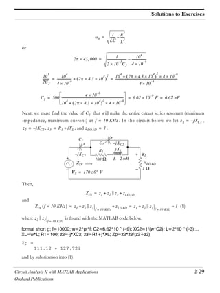
The expression of (2) will be minimum if we let at . Then, the
capacitor value must be such that or
Shown below is the plot of versus frequency and the MATLAB code that produces this
plot.
f=1000: 100: 60000; w=2*pi*f; Vs=170; C1=1.25*10^( 7); C2=6.62*10^( 9);...
L=2.*10.^( 3);...
R1=100; Rload=1; z1= j./(w.*C1); z2= j./(w.*C2); z3=R1+j.*w.*L; Zload=Rload;...
Zin=z1+z2.*z3./(z2+z3); Vload=Zload.*Vs./(Zin+Zload); magVload=abs(Vload);...
plot(f,magVload); axis([1000 60000 0 2]);...
xlabel('Frequency f'); ylabel('|Vload|'); grid
This circuit is considered to be a special type of filter that allows a specific frequency (not a band
of frequencies) to pass, and attenuates another specific frequency.
ZIN f 10 KHz= z1 111.12 j127.72 1+ + + z1 113.12+ j127.72+= =
z1 j127.72–= f 10 KHz=
C1 1 C 127.72=
C1
1
2 10
4
127.72
-------------------------------------------- 1.25 10
7–
F 0.125 F= = =
VLOAD

97. Circuit Analysis II with MATLAB Applications 3-1
Orchard Publications
Chapter 3
Elementary Signals
his chapter begins with a discussion of elementary signals that may be applied to electric net-
works. The unit step, unit ramp, and delta functions are then introduced. The sampling and
sifting properties of the delta function are defined and derived. Several examples for expressing
a variety of waveforms in terms of these elementary signals are provided.
3.1 Signals Described in Math Form
Consider the network of Figure 3.1 where the switch is closed at time .
Figure 3.1. A switched network with open terminals.
We wish to describe in a math form for the time interval . To do this, it is conve-
nient to divide the time interval into two parts, , and .
For the time interval the switch is open and therefore, the output voltage is zero. In
other words,
(3.1)
For the time interval the switch is closed. Then, the input voltage appears at the output,
i.e.,
(3.2)
Combining (3.1) and (3.2) into a single relationship, we get
(3.3)
We can express (3.3) by the waveform shown in Figure 3.2.
T
t 0=
+
+
vout
vS
t 0=
R
open terminals
vout t +–
t 0– 0 t
t 0– vout
vout 0 for t 0–=
0 t vS
vout vS for 0 t=
vout
0 – t 0
vS 0 t
=

98. Chapter 3 Elementary Signals
3-2 Circuit Analysis II with MATLAB Applications
Orchard Publications
Figure 3.2. Waveform for as defined in relation (3.3)
The waveform of Figure 3.2 is an example of a discontinuous function. A function is said to be dis-
continuous if it exhibits points of discontinuity, that is, the function jumps from one value to another
without taking on any intermediate values.
3.2 The Unit Step Function
A well-known discontinuous function is the unit step function *
that is defined as
(3.4)
It is also represented by the waveform of Figure 3.3.
Figure 3.3. Waveform for
In the waveform of Figure 3.3, the unit step function changes abruptly from to at .
But if it changes at instead, it is denoted as . Its waveform and definition are as
shown in Figure 3.4 and relation (3.5).
Figure 3.4. Waveform for
* In some books, the unit step function is denoted as , that is, without the subscript 0. In this text, however, we
will reserve the designation for any input.
0
voutvS
t
vout
u0 t
u0 t
u t
u t
u0 t
0 t 0
1 t 0
=
u0 t
0
1
t
u0 t
u0 t 0 1 t 0=
t t0= u0 t t0–
1
t00
u0 t t0–
t
u0 t t0–

99. Circuit Analysis II with MATLAB Applications 3-3
Orchard Publications
The Unit Step Function
(3.5)
If the unit step function changes abruptly from to at , it is denoted as . Its
waveform and definition are as shown in Figure 3.5 and relation (3.6).
Figure 3.5. Waveform for
(3.6)
Example 3.1
Consider the network of Figure 3.6, where the switch is closed at time .
Figure 3.6. Network for Example 3.1
Express the output voltage as a function of the unit step function, and sketch the appropriate
waveform.
Solution:
For this example, the output voltage for , and for . Therefore,
(3.7)
and the waveform is shown in Figure 3.7.
u0 t t0–
0 t t0
1 t t0
=
0 1 t t0–= u0 t t0+
tt0 0
1
u0 t t0+
u0 t t0+
u0 t t0+
0 t t0–
1 t t0–
=
t T=
+
+
vout
vS
t T=
R
open terminals
vout
vout 0= t T vout vS= t T
vout vSu0 t T–=

100. Chapter 3 Elementary Signals
3-4 Circuit Analysis II with MATLAB Applications
Orchard Publications
Figure 3.7. Waveform for Example 3.1
Other forms of the unit step function are shown in Figure 3.8.
Figure 3.8. Other forms of the unit step function
Unit step functions can be used to represent other time-varying functions such as the rectangular
pulse shown in Figure 3.9.
Figure 3.9. A rectangular pulse expressed as the sum of two unit step functions
Thus, the pulse of Figure 3.9(a) is the sum of the unit step functions of Figures 3.9(b) and 3.9(c) is
represented as .
T
t
0
vSu0 t T–
vout
0
t
t
t t
0
00
0
0
0
t
tt
0 0
t t
(a) (b) (c)
(d) (e) (f)
(g) (h) (i)
A A A
A A A
A A A
Au0 t–
A– u0 t A– u0 t T– A– u0 t T+
Au0 t– T+ Au0 t– T–
A– u0 t– A– u0 t– T+ A– u0 t– T–
0 0 0
t t t
1
1
1
u0 t
u0 t 1––
a b
c
u0 t u0 t 1––

101. Circuit Analysis II with MATLAB Applications 3-5
Orchard Publications
The Unit Step Function
The unit step function offers a convenient method of describing the sudden application of a voltage
or current source. For example, a constant voltage source of applied at , can be denoted
as . Likewise, a sinusoidal voltage source that is applied to a circuit at
, can be described as . Also, if the excitation in a circuit is a rect-
angular, or triangular, or sawtooth, or any other recurring pulse, it can be represented as a sum (dif-
ference) of unit step functions.
Example 3.2
Express the square waveform of Figure 3.10 as a sum of unit step functions. The vertical dotted lines
indicate the discontinuities at and so on.
Figure 3.10. Square waveform for Example 3.2
Solution:
Line segment has height , starts at , and terminates at . Then, as in Example 3.1, this
segment is expressed as
(3.8)
Line segment has height , starts at and terminates at . This segment is expressed
as
(3.9)
Line segment has height , starts at and terminates at . This segment is expressed as
(3.10)
Line segment has height , starts at , and terminates at . It is expressed as
(3.11)
Thus, the square waveform of Figure 3.10 can be expressed as the summation of (3.8) through (3.11),
that is,
24 V t 0=
24u0 t V v t Vm t Vcos=
t t0= v t Vm tcos u0 t t0– V=
T 2T 3T
t
v t
3T
A
0
A–
T 2T
A t 0= t T=
v1 t A u0 t u0 t T––=
A– t T= t 2T=
v2 t A– u0 t T– u0 t 2T––=
A t 2T= t 3T=
v3 t A u0 t 2T– u0 t 3T––=
A– t 3T= t 4T=
v4 t A– u0 t 3T– u0 t 4T––=

102. Chapter 3 Elementary Signals
3-6 Circuit Analysis II with MATLAB Applications
Orchard Publications
(3.12)
Combining like terms, we get
(3.13)
Example 3.3
Express the symmetric rectangular pulse of Figure 3.11 as a sum of unit step functions.
Figure 3.11. Symmetric rectangular pulse for Example 3.3
Solution:
This pulse has height , starts at , and terminates at . Therefore, with reference to
Figures 3.5 and 3.8 (b), we get
(3.14)
Example 3.4
Express the symmetric triangular waveform of Figure 3.12 as a sum of unit step functions.
Figure 3.12. Symmetric triangular waveform for Example 3.4
Solution:
We first derive the equations for the linear segments and shown in Figure 3.13.
v t v1 t v2 t v3 t v4 t+ + +=
A u0 t u0 t T–– A– u0 t T– u0 t 2T––=
+A u0 t 2T– u0 t 3T–– A– u0 t 3T– u0 t 4T––
v t A u0 t 2u0 t T–– 2u0 t 2T– 2u0 t 3T––+ +=
t
A
T– 2 T 20
i t
A t T 2–= t T 2=
i t Au0 t
T
2
---+ Au0 t
T
2
---–– A u0 t
T
2
---+ u0 t
T
2
---––= =
t
1
0T 2–
v t
T 2

103. Circuit Analysis II with MATLAB Applications 3-7
Orchard Publications
The Unit Step Function
Figure 3.13. Equations for the linear segments of Figure 3.12
For line segment ,
(3.15)
and for line segment ,
(3.16)
Combining (3.15) and (3.16), we get
(3.17)
Example 3.5
Express the waveform of Figure 3.14 as a sum of unit step functions.
Figure 3.14. Waveform for Example 3.5.
Solution:
As in the previous example, we first find the equations of the linear segments and shown in Fig-
ure 3.15.
t
1
0T 2–
v t
T 2
2
T
---– t 1+
2
T
--- t 1+
v1 t
2
T
--- t 1+ u0 t
T
2
---+ u0 t–=
v2 t
2
T
---– t 1+ u0 t u0 t
T
2
---––=
v t v1 t v2 t+=
2
T
--- t 1+ u0 t T
2
---+ u0 t– 2
T
---– t 1+ u0 t u0 t T
2
---––+=
1
2
3
1 2 30
t
v t

104. Chapter 3 Elementary Signals
3-8 Circuit Analysis II with MATLAB Applications
Orchard Publications
Figure 3.15. Equations for the linear segments of Figure 3.14
Following the same procedure as in the previous examples, we get
Multiplying the values in parentheses by the values in the brackets, we get
or
and combining terms inside the brackets, we get
(3.18)
Two other functions of interest are the unit ramp function, and the unit impulse or delta function. We
will introduce them with the examples that follow.
Example 3.6
In the network of Figure 3.16, where is a constant source, the switch is closed at time .
Figure 3.16. Network for Example 3.6
1
2
3
1 2 30
2t 1+
v t
t
t– 3+
v t 2t 1+ u0 t u0 t 1–– 3 u0 t 1– u0 t 2––+=
+ t– 3+ u0 t 2– u0 t 3––
v t 2t 1+ u0 t 2t 1+ u0 t 1–– 3u0 t 1–+=
3u0 t 2–– t– 3+ u0 t 2– t– 3+ u0 t 3––+
v t 2t 1+ u0 t 2t 1+– 3+ u0 t 1–+=
+ 3– t– 3++ u0 t 2– t– 3+ u0 t 3––
v t 2t 1+ u0 t 2 t 1– u0 t 1–– t– u0 t 2– t 3– u0 t 3–+=
iS t 0=
vC t
t 0=iS
R
C
+

105. Circuit Analysis II with MATLAB Applications 3-9
Orchard Publications
The Unit Step Function
Express the capacitor voltage as a function of the unit step.
Solution:
The current through the capacitor is , and the capacitor voltage is
* (3.19)
where is a dummy variable.
Since the switch closes at , we can express the current as
(3.20)
and assuming that for , we can write (3.19) as
(3.21)
or
(3.22)
Therefore, we see that when a capacitor is charged with a constant current, the voltage across it is a
linear function and forms a ramp with slope as shown in Figure 3.17.
Figure 3.17. Voltage across a capacitor when charged with a constant current source.
* Since the initial condition for the capacitor voltage was not specified, we express this integral with at the
lower limit of integration so that any non-zero value prior to would be included in the integration.
vC t
iC t iS cons ttan= = vC t
vC t
1
C
---- iC d
–
t
=
–
t 0
t 0= iC t
iC t iS u0 t=
vC t 0= t 0
vC t
1
C
---- iS u0 d
–
t
iS
C
---- u0 d
–
0
0
iS
C
---- u0 d
0
t
+= =
vC t
iS
C
----- tu0 t=
iS C
vC t
0
slope iS C=
t

106. Chapter 3 Elementary Signals
3-10 Circuit Analysis II with MATLAB Applications
Orchard Publications
3.3 The Unit Ramp Function
The unit ramp function, denoted as , is defined as
(3.23)
where is a dummy variable.
We can evaluate the integral of (3.23) by considering the area under the unit step function from
as shown in Figure 3.18.
Figure 3.18. Area under the unit step function from
Therefore, we define as
(3.24)
Since is the integral of , then must be the derivative of , i.e.,
(3.25)
Higher order functions of can be generated by repeated integration of the unit step function. For
example, integrating twice and multiplying by 2, we define as
(3.26)
Similarly,
(3.27)
and in general,
u1 t
u1 t
u1 t u0 d
–
t
=
u0 t
to t–
Area 1 t= = =
1
t
to t–
u1 t
u1 t
0 t 0
t t 0
=
u1 t u0 t u0 t u1 t
d
dt
-----u1 t u0 t=
t
u0 t u2 t
u2 t
0 t 0
t
2
t 0
= or u2 t 2 u1 d
–
t
=
u3 t
0 t 0
t
3
t 0
= or u3 t 3 u2 d
–
t
=

107. Circuit Analysis II with MATLAB Applications 3-11
Orchard Publications
The Unit Ramp Function
(3.28)
Also,
(3.29)
Example 3.7
In the network of Figure 3.19, the switch is closed at time and for .
Figure 3.19. Network for Example 3.7
Express the inductor current in terms of the unit step function.
Solution:
The voltage across the inductor is
(3.30)
and since the switch closes at ,
(3.31)
Therefore, we can write (3.30) as
(3.32)
But, as we know, is constant ( or ) for all time except at where it is discontinuous.
Since the derivative of any constant is zero, the derivative of the unit step has a non-zero value
only at . The derivative of the unit step function is defined in the next section.
un t
0 t 0
t
n
t 0
= or un t 3 un 1– d
–
t
=
un 1– t
1
n
---
d
dt
-----un t=
t 0= iL t 0= t 0
R
iS
t 0=
L
vL tiL t
+
iL t
vL t L
diL
dt
-------=
t 0=
iL t iS u0 t=
vL t LiS
d
dt
-----u0 t=
u0 t 0 1 t 0=
u0 t
t 0=

108. Chapter 3 Elementary Signals
3-12 Circuit Analysis II with MATLAB Applications
Orchard Publications
3.4 The Delta Function
The unit impulse or delta function, denoted as , is the derivative of the unit step . It is also
defined as
(3.33)
and
(3.34)
To better understand the delta function , let us represent the unit step as shown in Figure
3.20 (a).
Figure 3.20. Representation of the unit step as a limit.
The function of Figure 3.20 (a) becomes the unit step as . Figure 3.20 (b) is the derivative of
Figure 3.20 (a), where we see that as , becomes unbounded, but the area of the rectangle
remains . Therefore, in the limit, we can think of as approaching a very large spike or impulse
at the origin, with unbounded amplitude, zero width, and area equal to .
Two useful properties of the delta function are the sampling property and the sifting property.
3.5 Sampling Property of the Delta Function
The sampling property of the delta function states that
(3.35)
or, when ,
(3.36)
t
t u0 t
d
–
t
u0 t=
t 0 for all t 0=
t u0 t
1
2
Figure (a)
Figure (b)
Area =1
t
t
0
0
0
0 1 2
1 t
1
t
f t t a– f a t=
a 0=
f t t f 0 t=

109. Circuit Analysis II with MATLAB Applications 3-13
Orchard Publications
Sifting Property of the Delta Function
that is, multiplication of any function by the delta function results in sampling the function
at the time instants where the delta function is not zero. The study of discrete-time systems is based
on this property.
Proof:
Since then,
(3.37)
We rewrite as
(3.38)
Integrating (3.37) over the interval and using (3.38), we get
(3.39)
The first integral on the right side of (3.39) contains the constant term ; this can be written out-
side the integral, that is,
(3.40)
The second integral of the right side of (3.39) is always zero because
and
Therefore, (3.39) reduces to
(3.41)
Differentiating both sides of (3.41), and replacing with , we get
(3.42)
3.6 Sifting Property of the Delta Function
The sifting property of the delta function states that
f t t
t 0 for t 0 and t 0=
f t t 0 for t 0 and t 0=
f t
f t f 0 f t f 0–+=
to t–
f d
–
t
f 0 d
–
t
f f 0– d
–
t
+=
f 0
f 0 d
–
t
f 0 d
–
t
=
t 0 for t 0 and t 0=
f f 0– 0=
f 0 f 0– 0= =
f d
–
t
f 0 d
–
t
=
t
f t t f 0 t=
Sampling Property of t
t

110. Chapter 3 Elementary Signals
3-14 Circuit Analysis II with MATLAB Applications
Orchard Publications
(3.43)
that is, if we multiply any function by and integrate from , we will obtain the
value of evaluated at .
Proof:
Let us consider the integral
(3.44)
We will use integration by parts to evaluate this integral. We recall from the derivative of products
that
(3.45)
and integrating both sides we get
(3.46)
Now, we let ; then, . We also let ; then, . By substitu-
tion into (3.46), we get
(3.47)
We have assumed that ; therefore, for , and thus the first term of the
right side of (3.47) reduces to . Also, the integral on the right side is zero for , and there-
fore, we can replace the lower limit of integration by . We can now rewrite (3.47) as
and letting , we get
(3.48)
f t t – td
–
f=
f t t – to +–
f t t =
f t t – t where a bd
a
b
d xy xdy ydx or xdy+ d xy ydx–= =
x yd xy y xd–=
x f t= dx f t= dy t –= y u0 t –=
f t t – td
a
b
f t u0 t –
a
b
u0 t – f t td
a
b
–=
a b u0 t – 0= a
f b a
a
f t t – td
a
b
f b f t td
b
– f b f b f+–= =
a and b for any–
f t t – td
–
f=
Sifting Property of t

111. Circuit Analysis II with MATLAB Applications 3-15
Orchard Publications
Higher Order Delta Functions
3.7 Higher Order Delta Functions
An nth-order delta function is defined as the derivative of , that is,
(3.49)
The function is called doublet, is called triplet, and so on. By a procedure similar to the
derivation of the sampling property of the delta function, we can show that
(3.50)
Also, the derivation of the sifting property of the delta function can be extended to show that
(3.51)
Example 3.8
Evaluate the following expressions:
a.
b.
c.
Solution:
a. The sampling property states that For this example, and
. Then,
b. The sifting property states that . For this example, and .
Then,
c. The given expression contains the doublet; therefore, we use the relation
nth u0 t
n
t
n
dt
----- u0 t=
' t '' t
f t ' t a– f a ' t a– f ' a t a––=
f t
n
t – td
–
1–
n d
n
dt
n
-------- f t
t =
=
3t
4
t 1–
t t 2– td
–
t
2
' t 3–
f t t a– f a t a–= f t 3t
4
=
a 1=
3t
4
t 1– 3t
4
t 1=
t 1– 3 t 1–= =
f t t – td
–
f= f t t= 2=
t t 2– td
–
f 2 t t 2=
2= = =

112. Chapter 3 Elementary Signals
3-16 Circuit Analysis II with MATLAB Applications
Orchard Publications
Then, for this example,
Example 3.9
a. Express the voltage waveform shown in Figure 3.21 as a sum of unit step functions for the
time interval .
b. Using the result of part (a), compute the derivative of and sketch its waveform.
Figure 3.21. Waveform for Example 3.9
Solution:
a. We first derive the equations for the linear segments of the given waveform. These are shown in
Figure 3.22.
Next, we express in terms of the unit step function , and we get
(3.52)
Multiplying and collecting like terms in (3.52), we get
f t ' t a– f a ' t a– f ' a t a––=
t
2
' t 3– t
2
t 3=
' t 3–
d
dt
-----t
2
t 3=
t 3––=
9 ' t 3– 6 t 3––=
v t
1 t 7 s–
v t
1
2
1
1
2
3
1 2 3 4 5 6 7
0
V
t s
v t
v t u0 t
v t 2t u0 t 1+ u0 t 1–– 2 u0 t 1– u0 t 2––+=
+ t– 5+ u0 t 2– u0 t 4–– u0 t 4– u0 t 5––+
+ t– 6+ u0 t 5– u0 t 7––

113. Circuit Analysis II with MATLAB Applications 3-17
Orchard Publications
Higher Order Delta Functions
Figure 3.22. Equations for the linear segments of Figure 3.21
or
b. The derivative of is
(3.53)
From the given waveform, we observe that discontinuities occur only at , , and
. Therefore, , , and , and the terms that contain these
delta functions vanish. Also, by application of the sampling property,
and by substitution into (3.53), we get
1
2
1
1
2
3
1 2 3 4 5 6 7
0
v t
t– 6+
t– 5+
2t
t s
Vv t
v t 2tu0 t 1+ 2tu0 t 1–– 2u0 t 1–– 2u0 t 2–– tu0 t 2––=
+ 5u0 t 2– tu0 t 4– 5u0 t 4–– u0 t 4– u0 t 5––+ +
tu0 t 5– 6u0 t 5– tu0 t 7– 6u0 t 7––+ +–
v t 2tu0 t 1+ 2t– 2+ u0 t 1– t– 3+ u0 t 2–+ +=
+ t 4– u0 t 4– t– 5+ u0 t 5– t 6– u0 t 7–+ +
v t
dv
dt
------ 2u0 t 1+ 2t t 1+ 2u0 t 1–– 2t– 2+ t 1–+ +=
u0 t 2–– t– 3+ t 2– u0 t 4– t 4– t 4–+ + +
u0 t 5–– t– 5+ t 5– u0 t 7– t 6– t 7–+ + +
t 1–= t 2=
t 7= t 1– 0= t 4– 0= t 5– 0=
2t t 1+ 2t t 1–=
t 1+ 2 t 1+–= =
t– 3+ t 2– t– 3+ t 2=
t 2– t 2–= =
t 6– t 7– t 6– t 7=
t 7– t 7–= =

114. Chapter 3 Elementary Signals
3-18 Circuit Analysis II with MATLAB Applications
Orchard Publications
(3.54)
The plot of is shown in Figure 3.23.
Figure 3.23. Plot of the derivative of the waveform of Figure 3.23.
We observe that a negative spike of magnitude occurs at , and two positive spikes of
magnitude occur at , and . These spikes occur because of the discontinuities at
these points.
MATLAB* has built-in functions for the unit step, and the delta functions. These are denoted by the
names of the mathematicians who used them in their work. The unit step function is referred
to as Heaviside(t), and the delta function is referred to as Dirac(t). Their use is illustrated with
the examples below.
syms k a t; % Define symbolic variables
u=k*sym('Heaviside(t a)') % Create unit step function at t = a
u =
k*Heaviside(t-a)
d=diff(u) % Compute the derivative of the unit step function
d =
k*Dirac(t-a)
* An introduction to MATLAB®
is given in Appendix A.
dv
dt
------ 2u0 t 1+ 2– t 1+ 2u0 t 1– u0 t 2–––=
t 2– u0 t 4– u0 t 5–– u0 t 7– t 7–+ + + +
dv dt
1
1
1
2
1 2 3 4 5 6 70
2 t 1+–
dv
dt
------ V s
t 2– t 7–
t s
2 t 1–=
1 t 2= t 7=
u0 t
t

115. Circuit Analysis II with MATLAB Applications 3-19
Orchard Publications
Summary
int(d) % Integrate the delta function
ans =
Heaviside(t-a)*k
3.8 Summary
The unit step function that is defined as
The unit step function offers a convenient method of describing the sudden application of a volt-
age or current source.
The unit ramp function, denoted as , is defined as
The unit impulse or delta function, denoted as , is the derivative of the unit step . It is also
defined as
and
The sampling property of the delta function states that
or, when ,
The sifting property of the delta function states that
The sampling property of the doublet function states that
u0 t
u0 t
0 t 0
1 t 0
=
u1 t
u1 t u0 d
–
t
=
t u0 t
d
–
t
u0 t=
t 0 for all t 0=
f t t a– f a t=
a 0=
f t t f 0 t=
f t t – td
–
f=
' t
f t ' t a– f a ' t a– f ' a t a––=

116. Chapter 3 Elementary Signals
3-20 Circuit Analysis II with MATLAB Applications
Orchard Publications
3.9 Exercises
1. Evaluate the following functions:
a.
b.
c.
d.
e.
f.
2.
a. Express the voltage waveform shown in Figure 3.24, as a sum of unit step functions for
the time interval .
b. Using the result of part (a), compute the derivative of , and sketch its waveform.
Figure 3.24. Waveform for Exercise 2
tsin t
6
---–
2tcos t
4
---–
t
2
t
2
---–cos
2ttan t
8
---–
t
2
e
t–
t 2– td
–
t
2 1
t
2
---–sin
v t
0 t 7 s
v t
10
20
10
20
1 2 3 4 5 6 7
0
v t
t s
e
2t–
Vv t

117. Circuit Analysis II with MATLAB Applications 3-21
Orchard Publications
Solutions to Exercises
3.10 Solutions to Exercises
1. We apply the sampling property of the function for all expressions except (e) where we apply
the sifting property. For part (f) we apply the sampling property of the doublet.
We recall that the sampling property states that . Thus,
a.
b.
c.
d.
We recall that the sampling property states that . Thus,
e.
We recall that the sampling property for the doublet states that
Thus,
f.
2.
a.
or
t
f t t a– f a t a–=
tsin t
6
---– t t 6=
t
6
---–sin
6
--- t
6
---–sin 0.5 t
6
---–= = =
2tcos t
4
---– 2t t 4=
t
4
---–cos
2
--- t
4
---–cos 0= = =
t
2
t
2
---–cos
1
2
--- 1 2tcos+
t 2=
t
2
---–
1
2
--- 1 cos+ t
2
---–
1
2
--- 1 1– t
2
---– 0= = = =
2ttan t
8
---– 2t t 8=
tan t
8
---–
4
--- t
8
---–tan t
8
---–= = =
f t t – td
–
f=
t
2
e
t–
t 2– td
–
t
2
e
t–
t 2=
4e
2–
0.54= = =
f t ' t a– f a ' t a– f ' a t a––=
t
2 1
t
2
---–sin t t 2=
2 1
t
2
---–sin
d
dt
----- t t 2=
2
t
2
---–sin–=
1
2
--- 1 2tcos– t 2=
1
t
2
---– 2t t 2=
t
2
---–sin–=
1
2
--- 1 1+
1
t
2
---– t
2
---–sin–
1
t
2
---–==
v t e
2t–
u0 t u0 t 2–– 10t 30– u0 t 2– u0 t 3––+=
+ 10– t 50+ u0 t 3– u0 t 5–– 10t 70– u0 t 5– u0 t 7––+

118. Chapter 3 Elementary Signals
3-22 Circuit Analysis II with MATLAB Applications
Orchard Publications
b.
(1)
Referring to the given waveform we observe that discontinuities occur only at , ,
and . Therefore, and . Also, by the sampling property of the delta
function
and with these simplifications (1) above reduces to
The waveform for is shown below.
v t e
2t–
u0 t e
2t–
u0 t 2– 10tu0 t 2– 30u0 t 2– 10tu0 t 3– 30u0 t 3–+––+–=
10tu0 t 3–– 50u0 t 3– 10tu0 t 5– 50u0 t 5– 10tu0 t 5–+–+ +
70u0 t 5– 10tu0 t 7– 70u0 t 7–+––
e
2t–
u0 t e
2t–
10t 30–+– u0 t 2– 20t 80+– u0 t 3– 20t 120– u0 t 5–+ + +=
+ 10t 70+– u0 t 7–
dv
dt
------ 2e
2t–
u0 t e
2t–
t 2e
2t–
10+ u0 t 2– e
2t–
10t 30–+– t 2–+ + +–=
20u0 t 3– 20t– 80+ t 3– 20u0 t 5– 20t 120– t 5–+ + +–
10u0 t 7– 10t– 70+ t 7–+–
t 2= t 3=
t 5= t 0= t 7– 0=
e
2t–
10t 30–+– t 2– e
2t–
10t 30–+– t 2=
t 2–= 10 t 2––
20t– 80+ t 3– 20t– 80+ t 3=
t 3–= 20 t 3–=
20t 120– t 5– 20t 120– t 5=
t 5–= 20– t 5–=
dv dt 2e
2t–
u0 t 2e
2t–
u0 t 2– 10u0 t 2– 10 t 2––+ +–=
20u0 t 3– 20 t 3– 20u0 t 5– 20 t 5– 10u0 t 7–––+ +–
2e
2t–
u0 t u0 t 2–– 10 t 2– 10 u0 t 2– u0 t 3–– 20 t 3–+ +––=
10 u0 t 3– u0 t 5––– 20 t 5– 10 u0 t 5– u0 t 7––+–
dv dt
dv dt
20
10
V s
t s
20–
10–
1 2 3 4 5 6 7
10 t 2––
20 t 3–
20 t 5––
2e
2t–
–

119. Circuit Analysis II with MATLAB Applications 4-1
Orchard Publications
Chapter 4
The Laplace Transformation
his chapter begins with an introduction to the Laplace transformation, definitions, and proper-
ties of the Laplace transformation. The initial value and final value theorems are also discussed
and proved. It concludes with the derivation of the Laplace transform of common functions
of time, and the Laplace transforms of common waveforms.
4.1 Definition of the Laplace Transformation
The two-sided or bilateral Laplace Transform pair is defined as
(4.1)
(4.2)
where denotes the Laplace transform of the time function , denotes the
Inverse Laplace transform, and is a complex variable whose real part is , and imaginary part ,
that is, .
In most problems, we are concerned with values of time greater than some reference time, say
, and since the initial conditions are generally known, the two-sided Laplace transform
pair of (4.1) and (4.2) simplifies to the unilateral or one-sided Laplace transform defined as
(4.3)
(4.4)
The Laplace Transform of (4.3) has meaning only if the integral converges (reaches a limit), that is, if
(4.5)
To determine the conditions that will ensure us that the integral of (4.3) converges, we rewrite (4.5)
T
L f t F s= f t
–
e
st–
dt=
L
1–
F s f t=
1
2 j
-------- F s
j–
j+
e
st
ds=
L f t f t L
1–
F s
s
s j+=
t
t t0 0= =
L f t F= s f t
t0
e
st–
dt f t
0
e
st–
dt= =
L
1–
F s f= t
1
2 j
-------- F s
j–
j+
e
st
ds=
f t
0
e
st–
dt

120. Chapter 4 The Laplace Transformation
4-2 Circuit Analysis II with MATLAB Applications
Orchard Publications
as
(4.6)
The term in the integral of (4.6) has magnitude of unity, i.e., , and thus the condition
for convergence becomes
(4.7)
Fortunately, in most engineering applications the functions are of exponential order*. Then, we
can express (4.7) as,
(4.8)
and we see that the integral on the right side of the inequality sign in (4.8), converges if .
Therefore, we conclude that if is of exponential order, exists if
(4.9)
where denotes the real part of the complex variable .
Evaluation of the integral of (4.4) involves contour integration in the complex plane, and thus, it will
not be attempted in this chapter. We will see, in the next chapter, that many Laplace transforms can
be inverted with the use of a few standard pairs, and therefore, there is no need to use (4.4) to obtain
the Inverse Laplace transform.
In our subsequent discussion, we will denote transformation from the time domain to the complex
frequency domain, and vice versa, as
(4.10)
4.2 Properties of the Laplace Transform
1. Linearity Property
The linearity property states that if
have Laplace transforms
* A function is said to be of exponential order if .
f t e
t–
0
e
j t–
dt
e
j t–
e
j t–
1=
f t e
t–
0
dt
f t
f t f t ke
0t
for all t 0
f t e
t–
0
dt ke
0t
e
t–
0
dt
0
f t L f t
Re s 0=
Re s s
f t F s
f1 t f2 t fn t

121. Circuit Analysis II with MATLAB Applications 4-3
Orchard Publications
Properties of the Laplace Transform
respectively, and
are arbitrary constants, then,
(4.11)
Proof:
Note 1:
It is desirable to multiply by to eliminate any unwanted non-zero values of for .
2. Time Shifting Property
The time shifting property states that a right shift in the time domain by units, corresponds to mul-
tiplication by in the complex frequency domain. Thus,
(4.12)
Proof:
(4.13)
Now, we let ; then, and . With these substitutions, the second integral
on the right side of (4.13) becomes
3. Frequency Shifting Property
The frequency shifting property states that if we multiply some time domain function by an
exponential function where a is an arbitrary positive constant, this multiplication will produce a
shift of the s variable in the complex frequency domain by units. Thus,
F1 s F2 s Fn s
c1 c2 cn
c1 f1 t c2 f2 t cn fn t+ + + c1 F1 s c2 F2 s cn Fn s+ + +
L c1 f1 t c2 f2 t cn fn t+ + + c1 f1 t c2 f2 t cn fn t+ + +
t0
dt=
c1 f1 t
t0
e
st–
dt c2 f2 t
t0
e
st–
dt + cn fn t
t0
e
st–
dt+ +=
c1 F1 s c2 F2 s cn Fn s+ + +=
f t u0 t f t t 0
a
e
as–
f t a– u0 t a– e
as–
F s
L f t a– u0 t a– 0
0
a
e
st–
dt f t a–
a
e
st–
dt+=
t a– = t a+= dt d=
f
0
e
s a+–
d e
as–
f
0
e
s–
d e
as–
F s= =
f t
e
at–
a

122. Chapter 4 The Laplace Transformation
4-4 Circuit Analysis II with MATLAB Applications
Orchard Publications
(4.14)
Proof:
Note 2:
A change of scale is represented by multiplication of the time variable by a positive scaling factor
. Thus, the function after scaling the time axis, becomes .
4. Scaling Property
Let be an arbitrary positive constant; then, the scaling property states that
(4.15)
Proof:
and letting , we get
Note 3:
Generally, the initial value of is taken at to include any discontinuity that may be present
at . If it is known that no such discontinuity exists at , we simply interpret as .
5. Differentiation in Time Domain
The differentiation in time domain property states that differentiation in the time domain corresponds
to multiplication by in the complex frequency domain, minus the initial value of at .
Thus,
(4.16)
Proof:
e
at–
f t F s a+
L e
at–
f t e
at–
f t
0
e
st–
dt f t
0
e
s a+ t–
dt F s a+= = =
t
a f t f at
a
f at
1
a
---F
s
a
---
L f at f at
0
e
st–
dt=
t a=
L f at f
0
e
s a–
d
a
---
1
a
--- f
0
e
s a–
d
1
a
---F
s
a
---= = =
f t t 0=
t 0= t 0= f 0 f 0
s f t t 0=
f ' t
d
dt
----- f t= sF s f 0–
L f ' t f ' t
0
e
st–
dt=

123. Circuit Analysis II with MATLAB Applications 4-5
Orchard Publications
Properties of the Laplace Transform
Using integration by parts where
(4.17)
we let and . Then, , , and thus
The time differentiation property can be extended to show that
(4.18)
(4.19)
and in general
(4.20)
To prove (4.18), we let
and as we found above,
Then,
Relations (4.19) and (4.20) can be proved by similar procedures.
We must remember that the terms , and so on, represent the initial conditions.
Therefore, when all initial conditions are zero, and we differentiate a time function times,
this corresponds to multiplied by to the power.
v ud uv u vd–=
du f ' t= v e
st–
= u f t= dv se
st–
–=
L f ' t f t e
st–
0
s f t
0
e
st–
dt+ f t e
st–
0
a
a
lim sF s+= =
e
sa–
f a f 0–
a
lim sF s+ 0 f 0– sF s+==
d 2
dt
2
-------- f t s 2
F s sf 0– f ' 0–
d 3
dt
3
-------- f t s3
F s s2
f 0– sf ' 0– f '' 0–
d
n
dt
n
-------- f t s
n
F s s
n 1–
f 0– s
n 2–
f ' 0– f–
n 1–
0–
g t f ' t
d
dt
----- f t= =
L g ' t sL g t g 0–=
L f '' t sL f ' t f ' 0– s sL f t f 0– f ' 0–= =
s 2
F s sf 0– f ' 0–=
f 0 f ' 0 f '' 0
f t n
F s s nth

124. Chapter 4 The Laplace Transformation
4-6 Circuit Analysis II with MATLAB Applications
Orchard Publications
6. Differentiation in Complex Frequency Domain
This property states that differentiation in complex frequency domain and multiplication by minus one,
corresponds to multiplication of by in the time domain. In other words,
(4.21)
Proof:
Differentiating with respect to s, and applying Leibnitz’s rule* for differentiation under the integral, we
get
In general,
(4.22)
The proof for follows by taking the second and higher-order derivatives of with respect
to .
7. Integration in Time Domain
This property states that integration in time domain corresponds to divided by plus the initial
value of at , also divided by . That is,
(4.23)
* This rule states that if a function of a parameter is defined by the equation where f is some
known function of integration x and the parameter , a and b are constants independent of x and , and the par-
tial derivative exists and it is continuous, then .
f t t
tf t
d
ds
-----– F s
L f t F s f t
0
e
st–
dt= =
F f x xd
a
b
=
f
dF
d
-------
x
----------------- xd
a
b
=
d
ds
-----F s
d
ds
----- f t
0
e
st–
dt
s0
e
st–
f t dt t–
0
e
st–
f t dt= = =
tf t
0
e
st–
dt– L tf t–==
t
n
f t 1–
n d
n
ds
n
--------F s
n 2 F s
s
F s s
f t t 0= s
f
–
t
d F s
s
----------- f 0
s
------------+

125. Circuit Analysis II with MATLAB Applications 4-7
Orchard Publications
Properties of the Laplace Transform
Proof:
We express the integral of (4.23) as two integrals, that is,
(4.24)
The first integral on the right side of (4.24), represents a constant value since neither the upper, nor
the lower limits of integration are functions of time, and this constant is an initial condition denoted
as . We will find the Laplace transform of this constant, the transform of the second integral
on the right side of (4.24), and will prove (4.23) by the linearity property. Thus,
(4.25)
This is the value of the first integral in (4.24). Next, we will show that
We let
then,
and
Now,
(4.26)
and the proof of (4.23) follows from (4.25) and (4.26).
f
–
t
d f
–
0
d f
0
t
d+=
f 0
L f 0 f 0
0
e
st–
dt f 0 e
st–
0
dt f 0
e
st–
s–
--------
0
= = =
f 0 0
f 0
s
------------––
f 0
s
------------==
f
0
t
d
F s
s
-----------
g t f
0
t
d=
g' t f=
g 0 f
0
0
d 0= =
L g' t G s sL g t g 0– G s 0–= = =
sL g t G s=
L g t
G s
s
-----------=
L f
0
t
d F s
s
-----------=

126. Chapter 4 The Laplace Transformation
4-8 Circuit Analysis II with MATLAB Applications
Orchard Publications
8. Integration in Complex Frequency Domain
This property states that integration in complex frequency domain with respect to corresponds to
division of a time function by the variable , provided that the limit exists. Thus,
(4.27)
Proof:
Integrating both sides from to , we get
Next, we interchange the order of integration, i.e.,
and performing the inner integration on the right side integral with respect to , we get
9. Time Periodicity
The time periodicity property states that a periodic function of time with period corresponds to
the integral divided by in the complex frequency domain. Thus, if we let
be a periodic function with period , that is, , for we get the trans-
form pair
(4.28)
s
f t t f t
t
--------
t 0
lim
f t
t
-------- F s sd
s
F s f t
0
e
st–
dt=
s
F s sd
s
f t
0
e
st–
dt sd
s
=
F s sd
s
e
st–
s
sd f t td
0
=
s
F s sd
s
1
t
---– e
st–
s
f t td
0
f t
t
--------e
st–
td
0
L
f t
t
--------= = =
T
f t
0
T
e
st–
dt 1 e
sT–
– f t
T f t f t nT+= n 1 2 3=
f t nT+
f t
0
T
e
st–
dt
1 e
sT–
–
-----------------------------

127. Circuit Analysis II with MATLAB Applications 4-9
Orchard Publications
Properties of the Laplace Transform
Proof:
The Laplace transform of a periodic function can be expressed as
In the first integral of the right side, we let , in the second , in the third ,
and so on. The areas under each period of are equal, and thus the upper and lower limits of
integration are the same for each integral. Then,
(4.29)
Since the function is periodic, i.e., , we can write
(4.29) as
(4.30)
By application of the binomial theorem, that is,
(4.31)
we find that expression (4.30) reduces to
10. Initial Value Theorem
The initial value theorem states that the initial value of the time function can be found
from its Laplace transform multiplied by and letting .That is,
(4.32)
Proof:
From the time domain differentiation property,
or
L f t f t
0
e
st–
dt f t
0
T
e
st–
dt f t
T
2T
e
st–
dt f t
2T
3T
e
st–
dt+ + += =
t = t T+= t 2T+=
f t
L f t f
0
T
e
s–
d f T+
0
T
e
s T+–
d f 2T+
0
T
e
s 2T+–
d+ + +=
f f T+ f 2T+ f nT+= = = =
L f 1 e
sT–
e
2sT–
+ + + f
0
T
e
s–
d=
1 a a
2
a
3
+ + + +
1
1 a–
------------=
L f
f
0
T
e
s–
d
e
sT–
–
----------------------------------=
f 0 f t
s s
f t
t 0
lim sF s
s
lim f 0= =
d
dt
----- f t sF s f 0–

128. Chapter 4 The Laplace Transformation
4-10 Circuit Analysis II with MATLAB Applications
Orchard Publications
Taking the limit of both sides by letting , we get
Interchanging the limiting process, we get
and since
the above expression reduces to
or
11. Final Value Theorem
The final value theorem states that the final value of the time function can be found from
its Laplace transform multiplied by s, then, letting . That is,
(4.33)
Proof:
From the time domain differentiation property,
or
Taking the limit of both sides by letting , we get
L
d
dt
----- f t sF s f 0–
d
dt
----- f t
0
e
st–
dt= =
s
sF s f 0–
s
lim
d
dt
----- f t
T
e
st–
dt
T
0
lim
s
lim=
sF s f 0–
s
lim
d
dt
----- f t
T
e
st–
s
lim dt
T
0
lim=
e
st–
s
lim 0=
sF s f 0–
s
lim 0=
sF s
s
lim f 0=
f f t
s 0
f t
t
lim sF s
s 0
lim f= =
d
dt
----- f t sF s f 0–
L
d
dt
----- f t sF s f 0–
d
dt
----- f t
0
e
st–
dt= =
s 0

129. Circuit Analysis II with MATLAB Applications 4-11
Orchard Publications
Properties of the Laplace Transform
and by interchanging the limiting process, we get
Also, since
the above expression reduces to
and therefore,
12. Convolution in the Time Domain
Convolution*
in the time domain corresponds to multiplication in the complex frequency domain,
that is,
(4.34)
Proof:
(4.35)
We let ; then, , and . By substitution into (4.35),
* Convolution is the process of overlapping two signals. The convolution of two time functions and is
denoted as , and by definition, where is a dummy variable. It is
discussed in detail Signals and Systems with MATLAB Applications by this author.
sF s f 0–
s 0
lim
d
dt
----- f t
T
e
st–
dt
T
0
lim
s 0
lim=
sF s f 0–
s 0
lim
d
dt
----- f t
T
e
st–
s 0
lim dt
T
0
lim=
e
st–
s 0
lim 1=
sF s f 0–
s 0
lim
d
dt
----- f t
T
dt
T
0
lim f t
T
T
0
lim= =
f T f–
T
0
lim f f 0–==
sF s
s 0
lim f=
f1 t f2 t
f1 t *f2 t f1 t *f2 t f1 f2 t –
–
d=
f1 t *f2 t F1 s F2 s
L f1 t *f2 t L f1 f2 t –
–
d f1 f2 t –
0
d
0
e
st–
dt= =
f1 f2 t –
0
e
st–
dt
0
d=
t – = t += dt d=

130. Chapter 4 The Laplace Transformation
4-12 Circuit Analysis II with MATLAB Applications
Orchard Publications
13. Convolution in the Complex Frequency Domain
Convolution in the complex frequency domain divided by , corresponds to multiplication in the
time domain. That is,
(4.36)
Proof:
(4.37)
and recalling that the Inverse Laplace transform from (4.2) is
by substitution into (4.37), we get
We observe that the bracketed integral is ; therefore,
For easy reference, we have summarized the Laplace transform pairs and theorems in Table 4.1.
4.3 The Laplace Transform of Common Functions of Time
In this section, we will present several examples for finding the Laplace transform of common func-
tions of time.
Example 4.1
Find
L f1 t *f2 t f1 f2
0
e
s +–
d
0
d f1 e
s–
d
0
f2
0
e
s–
d= =
F1 s F2 s=
1 2 j
f1 t f2 t
1
2 j
-------- F1 s *F2 s
L f1 t f2 t f1 t f2 t
0
e
st–
dt=
f1 t
1
2 j
-------- F1
j–
j+
e
t
d=
L f1 t f2 t
1
2 j
-------- F1
j–
j+
e
t
d f2 t
0
e
st–
dt=
1
2 j
-------- F1
j–
j+
f2 t
0
e
s – t–
dt d=
F2 s –
L f1 t f2 t
1
2 j
-------- F1
j–
j+
F2 s – d
1
2 j
--------F1 s *F2 s= =
L u0 t

131. Circuit Analysis II with MATLAB Applications 4-13
Orchard Publications
The Laplace Transform of Common Functions of Time
TABLE 4.1 Summary of Laplace Transform Properties and Theorems
Property/Theorem Time Domain Complex Frequency Domain
1 Linearity
2 Time Shifting
3 Frequency Shifting
4 Time Scaling
5 Time Differentiation
See also (4.18) through (4.20)
6 Frequency Differentiation
See also (4.22)
7 Time Integration
8 Frequency Integration
9 Time Periodicity
10 Initial Value Theorem
11 Final Value Theorem
12 Time Convolution
13 Frequency Convolution
c1 f1 t c2 f2 t+
+ cn fn t+
c1 F1 s c2 F2 s+
+ cnFn s+
f t a– u0 t a–
e
as–
F s
e
as–
f t
F s a+
f at 1
a
---F
s
a
---
d
dt
----- f t sF s f 0–
tf t d
ds
-----– F s
f
–
t
d F s
s
-----------
f 0
s
------------+
f t
t
-------- F s sd
s
f t nT+
f t
0
T
e
st–
dt
1 e
sT–
–
--------------------------------
f t
t 0
lim
sF s
s
lim f 0=
f t
t
lim sF s
s 0
lim f=
f1 t *f2 t F1 s F2 s
f1 t f2 t 1
2 j
-------- F1 s *F2 s

132. Chapter 4 The Laplace Transformation
4-14 Circuit Analysis II with MATLAB Applications
Orchard Publications
Solution:
We start with the definition of the Laplace transform, that is,
For this example,
Thus, we have obtained the transform pair
(4.38)
for .*
Example 4.2
Find
Solution:
We apply the definition
and for this example,
We will perform integration by parts recalling that
(4.39)
We let
then,
By substitution into (4.39),
* This condition was established in (4.9).
L f t F s f t
0
e
st–
dt= =
L u0 t 1
0
e
st–
dt
e
st
–
s
---------
0
0
1
s
---––
1
s
---= = = =
u0 t
1
s
---
Re s 0=
L u1 t
L f t F s f t
0
e
st–
dt= =
L u1 t L t t
0
e
st–
dt= =
u vd uv v ud–=
u t and dv e
st–
= =
du 1 and v
e
st–
–
s
-----------= =

133. Circuit Analysis II with MATLAB Applications 4-15
Orchard Publications
The Laplace Transform of Common Functions of Time
(4.40)
Since the upper limit of integration in (4.40) produces an indeterminate form, we apply L’ Hôpital’s
rule*, that is,
Evaluating the second term of (4.40), we get
Thus, we have obtained the transform pair
(4.41)
for .
Example 4.3
Find
Solution:
To find the Laplace transform of this function, we must first review the gamma or generalized facto-
rial function defined as
(4.42)
* Often, the ratio of two functions, such as , for some value of x, say a, results in an indeterminate form. To
work around this problem, we consider the limit , and we wish to find this limit, if it exists. To find this
limit, we use L’Hôpital’s rule which states that if , and if the limit as x
approaches a exists, then,
L t
t– e
st–
s
-------------
0
e
st–
–
s
-----------
0
– dt t– e
st–
s
------------- e
st–
s
2
--------–
0
= =
f x
g x
----------
f x
g x
----------
x a
lim
f a g a 0= =
d
dx
------f x
d
dx
------g x
f x
g x
----------
x a
lim
d
dx
------f x
d
dx
------g x
x a
lim=
te
st–
t
lim t
e
st
------
t
lim td
d
t
td
d
e
st
----------------
t
lim 1
se
st
--------
t
lim 0= = = =
L t 1
s
2
----=
t
1
s2
----
0
L t
n
u0 t
n
n x
n 1–
e
x–
xd
0
=

134. Chapter 4 The Laplace Transformation
4-16 Circuit Analysis II with MATLAB Applications
Orchard Publications
The integral of (4.42) is an improper integral*
but converges (approaches a limit) for all .
We will now derive the basic properties of the gamma function, and its relation to the well known
factorial function
The integral of (4.42) can be evaluated by performing integration by parts. Thus, in (4.39) we let
Then,
and (4.42) is written as
(4.43)
With the condition that , the first term on the right side of (4.43) vanishes at the lower limit
. It also vanishes at the upper limit as . This can be proved with L’ Hôpital’s rule by dif-
ferentiating both numerator and denominator m times, where . Then,
Therefore, (4.43) reduces to
and with (4.42), we have
* Improper integrals are two types and these are:
a. where the limits of integration a or b or both are infinite
b. where f(x) becomes infinite at a value x between the lower and upper limits of integration inclusive.
n 0
f x xd
a
b
f x xd
a
b
n! n n 1– n 2– 3 2 1=
u e
x–
and dv x
n 1–
==
du e
x–
– dx and v x
n
n
-----==
n
x
n
e
x–
n
------------
x 0=
1
n
--- x
n
e
x–
xd
0
+=
n 0
x 0= x
m n
x
n
e
x–
n
------------
x
lim x
n
ne
x
--------
x
lim x
m
m
d
d
x
n
x
m
m
d
d
ne
x
-------------------
x
lim x
m 1–
m 1–
d
d
nx
n 1–
x
m 1–
m 1–
d
d
ne
x
------------------------------------
x
lim= = = =
n n 1– n 2– n m– 1+ x
n m–
ne
x
------------------------------------------------------------------------------------
x
lim n 1– n 2– n m– 1+
x
m n–
e
x
--------------------------------------------------------------------
x
lim 0= ==
n
1
n
--- x
n
e
x–
xd
0
=

135. Circuit Analysis II with MATLAB Applications 4-17
Orchard Publications
The Laplace Transform of Common Functions of Time
(4.44)
By comparing the integrals in (4.44), we observe that
(4.45)
or
(4.46)
It is convenient to use (4.45) for , and (4.46) for . From (4.45), we see that becomes
infinite as .
For , (4.42) yields
(4.47)
and thus we have the important relation,
(4.48)
From the recurring relation of (4.46), we obtain
(4.49)
and in general
(4.50)
for
The formula of (4.50) is a noteworthy relation; it establishes the relationship between the
function and the factorial
We now return to the problem of finding the Laplace transform pair for , that is,
(4.51)
To make this integral resemble the integral of the gamma function, we let , or , and
n x
n 1–
e
x–
xd
0
1
n
--- x
n
e
x–
xd
0
= =
n n 1+
n
---------------------=
n n n 1+=
n 0 n 0 n
n 0
n 1=
1 e
x–
xd
0
e
x–
0
– 1= = =
1 1=
2 1 1 1= =
3 2 2 2 1 2!= = =
4 3 3 3 2 3!= = =
n 1+ n!=
n 1 2 3=
n
n!
t
n
u0t
L t
n
u0t t
n
0
e
st–
dt=
st y= t y s=

136. Chapter 4 The Laplace Transformation
4-18 Circuit Analysis II with MATLAB Applications
Orchard Publications
thus . Now, we rewrite (4.51) as
Therefore, we have obtained the transform pair
(4.52)
for positive integers of and .
Example 4.4
Find
Solution:
and using the sifting property of the delta function, we get
Thus, we have the transform pair
(4.53)
for all .
Example 4.5
Find
Solution:
and again, using the sifting property of the delta function, we get
dt dy s=
L t
n
u0t
y
s
--
n
0
e
y–
d
y
s
--
1
s
n 1+
----------- y
n
0
e
y–
dy n 1+
s
n 1+
-------------------- n!
s
n 1+
-----------= = = =
t
n
u0 t
n!
s
n 1+
-----------
n 0
L t
L t t
0
e
st–
dt=
L t t
0
e
st–
dt e
s 0–
1= = =
t 1
L t a–
L t a– t a–
0
e
st–
dt=
L t a– t a–
0
e
st–
dt e
as–
= =

137. Circuit Analysis II with MATLAB Applications 4-19
Orchard Publications
The Laplace Transform of Common Functions of Time
Thus, we have the transform pair
(4.54)
for .
Example 4.6
Find
Solution:
Thus, we have the transform pair
(4.55)
for .
Example 4.7
Find
Solution:
For this example, we will use the transform pair of (4.52), i.e.,
(4.56)
and the frequency shifting property of (4.14), that is,
(4.57)
Then, replacing with in (4.56), we get the transform pair
t a– e
as–
0
L e
at–
u0 t
L e
at–
u0 t e
at–
0
e
st–
dt e
s a+ t–
0
dt==
1
s a+
-----------– e
s a+ t–
0
1
s a+
-----------==
e
at–
u0 t
1
s a+
-----------
a–
L t
n
e
at–
u0 t
t
n
u0 t
n!
s
n 1+
-----------
e
at–
f t F s a+
s s a+

138. Chapter 4 The Laplace Transformation
4-20 Circuit Analysis II with MATLAB Applications
Orchard Publications
(4.58)
where is a positive integer, and Thus, for , we get the transform pair
(4.59)
for .
For , we get the transform
(4.60)
and in general,
(4.61)
for
Example 4.8
Find
Solution:
and from tables of integrals*
Then,
* This can also be derived from , and the use of (4.55) where . By the lin-
earity property, the sum of these terms corresponds to the sum of their Laplace transforms. Therefore,
t
n
e
at–
u0 t
n!
s a+
n 1+
-------------------------
n a– n 1=
te
at–
u0 t
1
s a+
2
------------------
a–
n 2=
t
2
e
at–
u0 t
2!
s a+
3
------------------
t
n
e
at–
u0 t
n!
s a+
n 1+
-------------------------
a–
L t u0sin t
L t u0sin t tsin
0
e
st–
dt tsin
0
a
e
st–
dt
a
lim= =
tsin
1
j2
----- e
j t
e
j t–
–= e
at–
u0 t
1
s a+
-----------
L tu0sin t
1
j2
----- 1
s j–
--------------
1
s j+
--------------–
s2 2
+
-----------------= =
e
ax
bxsin dx e
ax
a bxsin b bxcos–
a
2
b
2
+
------------------------------------------------------=

139. Circuit Analysis II with MATLAB Applications 4-21
Orchard Publications
The Laplace Transform of Common Functions of Time
Thus, we have obtained the transform pair
(4.62)
for
Example 4.9
Find
Solution:
and from tables of integrals*
Then,
Thus, we have the fransform pair
* We can use the relation and the linearity property, as in the derivation of the transform
of on the footnote of the previous page. We can also use the transform pair ; this
is the time differentiation property of (4.16). Applying this transform pair for this derivation, we get
L t u0sin t e
st–
s– tsin tcos–
s
2 2
+
-----------------------------------------------------------
0
a
a
lim=
e
as–
s– asin acos–
s
2 2
+
--------------------------------------------------------------
s
2 2
+
-----------------+
a
lim
s
2 2
+
-----------------==
t u0tsin
s
2 2
+
-----------------
0
L cos t u0 t
L cos t u0 t tcos
0
e
st–
dt tcos
0
a
e
st–
dt
a
lim= =
tcos
1
2
--- e
j t
e
j t–
+=
sin t
d
dt
----- f t sF s f 0–
L cos tu0 t L
1
----
d
dt
-----sin tu0 t
1
----L
d
dt
-----sin tu0 t
1
----s
s2 2
+
----------------- s
s2 2
+
-----------------= = = =
e
ax
bxcos dx
e
ax
bxacos b bxsin+
a
2
b
2
+
------------------------------------------------------=
L cos t u0 t e
st–
s– tcos tsin+
s
2 2
+
-----------------------------------------------------------
0
a
a
lim=
e
as–
s– acos asin+
s
2 2
+
--------------------------------------------------------------- s
s
2 2
+
-----------------+
a
lim s
s
2 2
+
-----------------==

140. Chapter 4 The Laplace Transformation
4-22 Circuit Analysis II with MATLAB Applications
Orchard Publications
(4.63)
for
Example 4.10
Find
Solution:
Since
using the frequency shifting property of (4.14), that is,
(4.64)
we replace with , and we get
(4.65)
for and .
Example 4.11
Find
Solution:
Since
using the frequency shifting property of (4.14), we replace with , and we get
(4.66)
for and .
For easy reference, we have summarized the above derivations in Table 4.2.
cos t u0t
s
s
2 2
+
-----------------
0
L e
at–
t u0sin t
tu0tsin
s
2 2
+
-----------------
e
at–
f t F s a+
s s a+
e
at–
t u0sin t
s a+
2 2
+
-------------------------------
0 a 0
L e
at–
cos t u0 t
cos t u0 t
s
s
2 2
+
-----------------
s s a+
e
at–
cos t u0 t
s a+
s a+
2 2
+
-------------------------------
0 a 0

141. Circuit Analysis II with MATLAB Applications 4-23
Orchard Publications
The Laplace Transform of Common Waveforms
4.4 The Laplace Transform of Common Waveforms
In this section, we will present some examples for deriving the Laplace transform of several wave-
forms using the transform pairs of Tables 4.1 and 4.2.
Example 4.12
Find the Laplace transform of the waveform of Figure 4.1. The subscript stands for pulse.
TABLE 4.2 Laplace Transform Pairs for Common Functions
1
2
3
4
5
6
7
8
9
10
11
f t F s
u0 t 1 s
tu0 t 1 s
2
t
n
u0 t n!
s
n 1+
-----------
t 1
t a– e
as–
e
at–
u0 t 1
s a+
-----------
t
n
e
at–
u0 t
n!
s a+
n 1+
-------------------------
t u0 tsin
s
2 2
+
-----------------
cos t u0 t s
s
2 2
+
-----------------
e
at–
t u0 tsin
s a+
2 2
+
-------------------------------
e
at–
cos t u0 t s a+
s a+
2 2
+
-------------------------------
fP t P

142. Chapter 4 The Laplace Transformation
4-24 Circuit Analysis II with MATLAB Applications
Orchard Publications
Figure 4.1. Waveform for Example 4.12
Solution:
We first express the given waveform as a sum of unit step functions. Then,
(4.67)
Next, from Table 4.1,
and from Table 4.2,
For this example,
and
Then, by the linearity property, the Laplace transform of the pulse of Figure 4.1 is
Example 4.13
Find the Laplace transform for the waveform of Figure 4.4. The subscript stands for line.
Figure 4.2. Waveform for Example 4.13
A
a
t
0
fP t
fP t A u0 t u0 t a––=
f t a– u0 t a– e
as–
F s
u0 t 1 s
Au0 t A s
Au0 t a– e
as– A
s
---
A u0 t u0 t a––
A
s
--- e
as–
–
A
s
---
A
s
--- 1 e
as–
–=
fL t L
1
t
0
1
2
fL t

143. Circuit Analysis II with MATLAB Applications 4-25
Orchard Publications
The Laplace Transform of Common Waveforms
Solution:
We must first derive the equation of the linear segment. This is shown in Figure 4.3. Then, we
express the given waveform in terms of the unit step function.
Figure 4.3. Waveform for Example 4.13 with the equation of the linear segment
For this example,
From Table 4.1,
and from Table 4.2,
Therefore, the Laplace transform of the linear segment of Figure 4.2 is
(4.68)
Example 4.14
Find the Laplace transform for the triangular waveform of Figure 4.4.
Solution:
We must first derive the equations of the linear segments. These are shown in Figure 4.5. Then, we
express the given waveform in terms of the unit step function.
Figure 4.4. Waveform for Example 4.14
1
t
0
1
2
fL t t 1–
fL t t 1– u0 t 1–=
f t a– u0 t a– e
as–
F s
tu0 t
1
s
2
----
t 1– u0 t 1– e
s– 1
s2
----
fT t
1
t
0
1
2
fT t

144. Chapter 4 The Laplace Transformation
4-26 Circuit Analysis II with MATLAB Applications
Orchard Publications
Figure 4.5. Waveform for Example 4.13 with the equations of the linear segments
For this example,
and collecting like terms,
From Table 4.1,
and from Table 4.2,
Then,
or
Therefore, the Laplace transform of the triangular waveform of Figure 4.3 is
(4.69)
Example 4.15
Find the Laplace transform for the rectangular periodic waveform of Figure 4.6.
1
t
0
1
2
fT t
t– 2+
t
fT t t u0 t u0 t 1–– t– 2+ u0 t 1– u0 t 2––+=
tu0 t tu0 t 1–– tu0 t 1–– 2u0 t 1– tu0 t 2– 2u0 t 2––+ +=
fT t tu0 t 2 t 1– u0 t 1– t 2– u0 t 2–+–=
f t a– u0 t a– e
as–
F s
tu0 t
1
s
2
----
tu0 t 2 t 1– u0 t 1– t 2– u0 t 2–+– 1
s
2
---- 2e–
s– 1
s
2
---- e
2s– 1
s
2
----+
tu0 t 2 t 1– u0 t 1– t 2– u0 t 2–+–
1
s
2
---- 1 2e
s–
– e
2s–
+
fT t
1
s
2
---- 1 e
s–
–
2
fR t

145. Circuit Analysis II with MATLAB Applications 4-27
Orchard Publications
The Laplace Transform of Common Waveforms
Figure 4.6. Waveform for Example 4.15
Solution:
This is a periodic waveform with period , and thus we can apply the time periodicity prop-
erty
where the denominator represents the periodicity of . For this example,
or
or
(4.70)
a
t
0
A
2a 3a
A
fR t
T 2a=
L f
f
0
T
e
s–
d
1 e
sT–
–
-------------------------------=
f t
L fR t
1
1 e
2as–
–
--------------------- fR t
0
2a
e
st–
dt
1
1 e
2as–
–
--------------------- A
0
a
e
st–
dt A–
a
2a
e
st–
dt+= =
A
1 e
2as–
–
--------------------- e
st–
–
s
-----------
0
a
e
st–
s
--------
a
2a
+=
L fR t
A
s 1 e
2as–
–
---------------------------- e
as–
– 1 e
2as–
e
as–
–+ +=
A
s 1 e
2as–
–
---------------------------- 1 2e
as–
– e
2as–
+
A 1 e
as–
–
2
s 1 e
as–
+ 1 e
as–
–
--------------------------------------------------==
A
s
---
1 e
as–
–
1 e
as–
+
-----------------------
A
s
---
e
as 2
e
as 2–
e
as 2–
e
as 2–
–
e
as 2
e
as 2–
e
as 2–
e
as 2–
+
---------------------------------------------------------------==
A
s
---
e
as 2–
e
as 2–
--------------
e
as 2
e
as 2–
–
e
as 2
e
as 2–
+
---------------------------------
A
s
---
as 2sinh
as 2cosh
-----------------------------==
fR t
A
s
---
as
2
-----tanh

146. Chapter 4 The Laplace Transformation
4-28 Circuit Analysis II with MATLAB Applications
Orchard Publications
Example 4.16
Find the Laplace transform for the half-rectified sine wave of Figure 4.7.
Figure 4.7. Waveform for Example 4.16
Solution:
This is a periodic waveform with period . We will apply the time periodicity property
where the denominator represents the periodicity of . For this example,
or
(4.71)
fHW t
sint
1
2 3 4
fHW t
T 2=
L f
f
0
T
e
s–
d
1 e
sT–
–
-------------------------------=
f t
L fHW t
1
1 e
2 s–
–
--------------------- f t
0
2
e
st–
dt
1
1 e
2 s–
–
--------------------- tsin
0
e
st–
dt= =
1
1 e
2 s–
–
--------------------- e
st–
s t tcos–sin
s
2
1+
------------------------------------------
0
1
s
2
1+
------------------ 1 e
s–
+
1 e
2 s–
–
--------------------------==
L fHW t
1
s
2
1+
------------------
1 e
s–
+
1 e
s–
+ 1 e
s–
–
-----------------------------------------------=
fHW t
1
s
2
1+ 1 e
s–
–
------------------------------------------

147. Circuit Analysis II with MATLAB Applications 4-29
Orchard Publications
Summary
4.5 Summary
The two-sided or bilateral Laplace Transform pair is defined as
where denotes the Laplace transform of the time function , denotes
the Inverse Laplace transform, and is a complex variable whose real part is , and imaginary
part , that is, .
The unilateral or one-sided Laplace transform defined as
We denote transformation from the time domain to the complex frequency domain, and vice
versa, as
The linearity property states that
The time shifting property states that
The frequency shifting property states that
The scaling property states that
The differentiation in time domain property states that
L f t F s= f t
–
e
st–
dt=
L
1–
F s f t=
1
2 j
-------- F s
j–
j+
e
st
ds=
L f t f t L
1–
F s
s
s j+=
L f t F= s f t
t0
e
st–
dt f t
0
e
st–
dt= =
f t F s
c1 f1 t c2 f2 t cn fn t+ + + c1 F1 s c2 F2 s cn Fn s+ + +
f t a– u0 t a– e
as–
F s
e
at–
f t F s a+
f at
1
a
---F
s
a
---
f ' t
d
dt
----- f t= sF s f 0–

148. Chapter 4 The Laplace Transformation
4-30 Circuit Analysis II with MATLAB Applications
Orchard Publications
and in general
where the terms , and so on, represent the initial conditions.
The differentiation in complex frequency domain property states that
and in general,
The integration in time domain property states that
The integration in complex frequency domain property states that
provided that the limit exists.
The time periodicity property states that
The initial value theorem states that
d 2
dt
2
-------- f t s 2
F s sf 0– f ' 0–
d 3
dt
3
-------- f t s3
F s s2
f 0– sf ' 0– f '' 0–
d
n
dt
n
-------- f t s
n
F s s
n 1–
f 0– s
n 2–
f ' 0– f–
n 1–
0–
f 0 f ' 0 f '' 0
tf t
d
ds
-----– F s
t
n
f t 1–
n d
n
ds
n
--------F s
f
–
t
d
F s
s
-----------
f 0
s
------------+
f t
t
-------- F s sd
s
f t
t
--------
t 0
lim
f t nT+
f t
0
T
e
st–
dt
1 e
sT–
–
-----------------------------
f t
t 0
lim sF s
s
lim f 0= =

149. Circuit Analysis II with MATLAB Applications 4-31
Orchard Publications
Summary
The final value theorem states that
Convolution in the time domain corresponds to multiplication in the complex frequency domain,
that is,
Convolution in the complex frequency domain divided by , corresponds to multiplication
in the time domain. That is,
The Laplace transforms of some common functions of time are shown below.
f t
t
lim sF s
s 0
lim f= =
f1 t *f2 t F1 s F2 s
1 2 j
f1 t f2 t
1
2 j
-------- F1 s *F2 s
u0 t 1 s
t 1 s2
t
n
u0 t
n!
s
n 1+
-----------
t 1
t a– e
as–
e
at–
u0 t
1
s a+
-----------
te
at–
u0 t
1
s a+
2
------------------
t
2
e
at–
u0 t
2!
s a+
3
------------------
t
n
e
at–
u0 t
n!
s a+
n 1+
-------------------------
t u0tsin
s
2 2
+
-----------------
cos t u0t
s
s
2 2
+
-----------------

150. Chapter 4 The Laplace Transformation
4-32 Circuit Analysis II with MATLAB Applications
Orchard Publications
The Laplace transforms of some common waveforms are shown below.
e
at–
t u0sin t
s a+
2 2
+
-------------------------------
e
at–
cos t u0 t
s a+
s a+
2 2
+
-------------------------------
A
a
t
0
fP t
A u0 t u0 t a––
A
s
--- e
as–
–
A
s
---
A
s
--- 1 e
as–
–=
1
t
0
1
2
fL t
t 1– u0 t 1– e
s– 1
s2
----
1
t
0
1
2
fT t
fT t
1
s
2
---- 1 e
s–
–
2
a
t
0
A
2a 3a
A
fR t
fR t
A
s
---
as
2
-----tanh

151. Circuit Analysis II with MATLAB Applications 4-33
Orchard Publications
Summary
sint
1
2 3 4
fHW t
fHW t
1
s
2
1+ 1 e
s–
–
------------------------------------------

152. Chapter 4 The Laplace Transformation
4-34 Circuit Analysis II with MATLAB Applications
Orchard Publications
4.6 Exercises
1. Find the Laplace transform of the following time domain functions:
a.
b.
c.
d.
e.
2. Find the Laplace transform of the following time domain functions:
a.
b.
c.
d.
e.
3. Find the Laplace transform of the following time domain functions:
a.
b.
c.
d.
e. Be careful with this! Comment and skip derivation.
4. Find the Laplace transform of the following time domain functions:
a.
b.
c.
12
6u0 t
24u0 t 12–
5tu0 t
4t
5
u0 t
j8
j5 90–
5e
5t–
u0 t
8t
7
e
5t–
u0 t
15 t 4–
t
3
3t
2
4t 3+ + + u0 t
3 2t 3– t 3–
3 5tsin u0 t
5 3tcos u0 t
2 4ttan u0 t
3t 5tsin u0 t
2t
2
3tcos u0 t
2e
5t–
5tsin

153. Circuit Analysis II with MATLAB Applications 4-35
Orchard Publications
Exercises
d.
e.
5. Find the Laplace transform of the following time domain functions:
a.
b.
c.
d.
e.
6. Find the Laplace transform of the following time domain functions:
a.
b.
c.
d.
e.
7. Find the Laplace transform of the following time domain functions:
a.
b.
c.
d.
8e
3t–
4tcos
tcos t 4–
5tu0 t 3–
2t
2
5t 4+– u0 t 3–
t 3– e
2t–
u0 t 2–
2t 4– e
2 t 2–
u0 t 3–
4te
3t–
2tcos u0 t
td
d
3tsin
td
d
3e
4t–
td
d
t
2
2tcos
td
d e
2t–
2tsin
td
d
t
2
e
2t–
tsin
t
---------
sin----------d
0
t
atsin
t
------------
cos
-----------d
t

154. Chapter 4 The Laplace Transformation
4-36 Circuit Analysis II with MATLAB Applications
Orchard Publications
e.
8. Find the Laplace transform for the sawtooth waveform of Figure 4.8.
Figure 4.8. Waveform for Exercise 8.
9. Find the Laplace transform for the full rectification waveform of Figure 4.9.
Figure 4.9. Waveform for Exercise 9
e
–
-------d
t
fST t
A
a 2a
t
fST t
3a
fFR t
Full Rectified Waveform
sint
1
a 2a 3a 4a
fFR t

155. Circuit Analysis II with MATLAB Applications 4-37
Orchard Publications
Solutions to Exercises
4.7 Solutions to Exercises
1. From the definition of the Laplace transform or from Table 4.2 we get:
a. b. c. d. e.
2. From the definition of the Laplace transform or from Table 4.2 we get:
a. b. c. d. e.
3.
a. From Table 4.2 and the linearity property
b. and
c. d. e. . This answer looks sus-
picious because and the Laplace transform is unilateral, that is, there is one-to-
one correspondence between the time domain and the complex frequency domain. The fallacy
with this procedure is that if we assume that and , we cannot con-
clude that . For this exercise and as we’ve learned
multiplication in the time domain corresponds to convolution in the complex frequency
domain. Accordingly, we must use the Laplace transform definition and this
requires integration by parts. We skip this analytical derivation. The interested reader may try
to find the answer with the MATLAB code syms s t; 2*laplace(sin(4*t)/cos(4*t))
4. From (4.22)
Then,
a.
12 s 6 s e
12s– 24
s
------ 5 s
2
4
5!
s
6
-----
j8 s 5 s
5
s 5+
----------- 8
7!
s 5+
8
------------------ 15e
4s–
3!
s
4
-----
3 2!
s
3
--------------
4
s
2
----
3
s
---+ + +
3 2t 3– t 3– 3 2t 3– t 3=
t 3– 9 t 3–= = 9 t 3– 9e
3s–
3
5
s
2
5
2
+
---------------- 5
s
s
2
3
2
+
---------------- 2 4ttan 2
4tsin
4tcos
------------- 2
4 s
2
2
2
+
s s
2
2
2
+
---------------------------- 8
s
---==
8 s 8u0 t
f1 t F1 s f2 t F2 s
f1 t
f2 t
----------
F1 s
F2 s
------------- f1 t f2 t 4t
1
4tcos
-------------sin=
2 4ttan e
st–
td
0
t
n
f t 1–
n d
n
ds
n
--------F s
3 1–
1 d
ds
----- 5
s
2
5
2
+
---------------- 3
5 2s–
s
2
25+
2
------------------------–
30s
s
2
25+
2
------------------------= =

156. Chapter 4 The Laplace Transformation
4-38 Circuit Analysis II with MATLAB Applications
Orchard Publications
b.
c.
d.
e.
and
5.
a.
b.
c.
2 1–
2 d
2
ds
2
--------
s
s
2
3
2
+
---------------- 2
d
ds
-----
s
2
3
2
s 2s–+
s
2
9+
2
----------------------------------- 2
d
ds
-----
s
2
– 9+
s
2
9+
2
---------------------= =
2
s
2
9+
2
2s– 2 s
2
9+ 2s s
2
– 9+–
s
2
9+
4
--------------------------------------------------------------------------------------------------=
2
s
2
9+ 2s– 4s s
2
– 9+–
s
2
9+
3
-------------------------------------------------------------------- 2
2s
3
– 18s– 4s
3
36s–+
s
2
9+
3
--------------------------------------------------------==
2
2s
3
54s–
s
2
9+
3
---------------------- 2
2s s
2
27–
s
2
9+
3
--------------------------- 4s s
2
27–
s
2
9+
3
---------------------------= ==
2 5
s 5+
2
5
2
+
------------------------------ 10
s 5+
2
25+
-------------------------------=
8 s 3+
s 3+
2
4
2
+
------------------------------
8 s 3+
s 3+
2
16+
-------------------------------=
t 4
cos t 4– 2 2 t 4–= 2 2 t 4– 2 2 e
4 s–
5tu0 t 3– 5 t 3– 15+ u0 t 3– e
3s– 5
s
2
---- 15
s
------+
5
s
---e
3s– 1
s
--- 3+==
2t
2
5t 4+– u0 t 3– 2 t 3–
2
12t 18– 5t– 4+ + u0 t 3–=
2 t 3–
2
7t 14–+ u0 t 3–=
2 t 3–
2
7 t 3– 21 14–+ + u0 t 3–=
2 t 3–
2
7 t 3– 7+ + u0 t 3– e
3s– 2 2!
s
3
--------------
7
s
2
----
7
s
---+ +=
t 3– e
2t–
u0 t 2– t 2– 1– e
2 t 2––
e
4–
u0 t 2–=
e
4–
e
2s– 1
s 2+
2
------------------
1
s 2+
----------------– e
4–
e
2s– s 1+–
s 2+
2
-------------------=

157. Circuit Analysis II with MATLAB Applications 4-39
Orchard Publications
Solutions to Exercises
d.
e.
6.
a.
b.
c.
Thus,
2t 4– e
2 t 2–
u0 t 3– 2 t 3– 6 4–+ e
2 t 3––
e
2–
u0 t 3–=
e
2–
e
3s– 2
s 3+
2
------------------
2
s 3+
----------------+ 2e
2–
e
3s– s 4+
s 3+
2
------------------=
4te
3t–
2tcos u0 t 4 1–
1 d
ds
-----
s 3+
s 3+
2
2
2
+
------------------------------ 4–
d
ds
-----
s 3+
s
2
6s 9 4+ + +
-----------------------------------=
4–
d
ds
-----
s 3+
s
2
6s 13+ +
----------------------------- 4
s
2
6s 13 s 3+ 2s 6+–+ +
s
2
6s 13+ +
2
------------------------------------------------------------------------–=
4
s
2
6s 13 2s
2
– 6s– 6s– 18–+ +
s
2
6s 13+ +
2
------------------------------------------------------------------------------ 4 s
2
6s 5+ +
s
2
6s 13+ +
2
------------------------------------=–
3t
3
s
2
3
2
+
----------------sin
d
dt
-----f t sF s f 0– f 0 3tsin t 0=
0= =
td
d
3tsin s
3
s
2
3
2
+
---------------- 0–
3s
s
2
9+
--------------=
3e
4t– 3
s 4+
-----------
d
dt
-----f t sF s f 0– f 0 3e
4t–
t 0=
3= =
td
d
3e
4t–
s
3
s 4+
----------- 3–
3s
s 4+
-----------
3 s 4+
s 4+
-------------------–
12–
s 4+
-----------= =
2tcos
s
s
2
2
2
+
---------------- t
2
2tcos 1–
2 d
2
ds
2
--------
s
s
2
4+
--------------
d
ds
----- s
2
4 s 2s–+
s
2
4+
2
--------------------------------- d
ds
----- s–
2
4+
s
2
4+
2
--------------------- s
2
4+
2
2s– s–
2
4+ s
2
4+ 2 2s–
s
2
4+
4
-------------------------------------------------------------------------------------------------= =
s
2
4+ 2s– s–
2
4+ 4s–
s
2
4+
3
------------------------------------------------------------------------
2s
3
– 8s– 4s
3
16s–+
s
2
4+
3
-----------------------------------------------------
2s s
2
12–
s
2
4+
3
---------------------------= ==
t
2
2tcos
2s s
2
12–
s
2
4+
3
---------------------------

158. Chapter 4 The Laplace Transformation
4-40 Circuit Analysis II with MATLAB Applications
Orchard Publications
and
d.
e.
7.
a.
but to find we must show that the limit exists. Since
this condition is satisfied and thus . From tables of integrals
. Then, and the constant of inte-
gration is evaluated from the final value theorem. Thus,
and
b.
From (a) above and since , it follows that
td
d t
2
2tcos sF s f 0–
s
2s s
2
12–
s
2
4+
3
--------------------------- 0–
2s
2
s
2
12–
s
2
4+
3
------------------------------=
2sin t
2
s
2
2
2
+
---------------- e
2t–
2tsin
2
s 2+
2
4+
----------------------------
d
dt
-----f t sF s f 0–
td
d e
2t–
2tsin s
2
s 2+
2
4+
---------------------------- 0– 2s
s 2+
2
4+
----------------------------=
t
2 2!
s
3
----- t
2
e
2t– 2!
s 2+
3
------------------ d
dt
-----f t sF s f 0–
td
d
t
2
e
2t–
s
2!
s 2+
3
------------------ 0–
2s
s 2+
3
------------------=
tsin
1
s
2
1+
-------------- L
tsin
t
--------- tsin
t
---------
t 0
lim
xsin
x
----------
x 0
lim 1=
tsin
t
---------
1
s
2
1+
-------------- sd
s
1
x
2
a
2
+
---------------- xd
1
a
--- x a
1–
tan C+=
1
s
2
1+
-------------- sd 1 s
1–
tan= C+
C
f t
t
lim sF s
s 0
lim s 1 s
1–
tan C+
s 0
lim 0= = =
tsin
t
--------- 1 s
1–
tan
tsin
t
--------- 1 s
1–
tan f
–
t
d F s
s
----------- f 0
s
------------+
sin----------
0
t
d
1
s
--- 1 s
1–
tan

159. Circuit Analysis II with MATLAB Applications 4-41
Orchard Publications
Solutions to Exercises
c.
From (a) above and since , it follows that
or
d.
, , and from tables of integrals
. Then, and the constant of inte-
gration is evaluated from the final value theorem. Thus,
and using we
get
e.
, , and from tables of integrals
. Then, and the constant of integration
is evaluated from the final value theorem. Thus,
and using we
get
8.
This is a periodic waveform with period and its Laplace transform is
tsin
t
--------- 1 s
1–
tan f at
1
a
---F
s
a
---
atsin
at
------------
1
a
---
1 s
a
---------
1–
tan
atsin
t
------------ a s
1–
tan
tcos
s
s
2
1+
-------------- tcos
t
---------- s
s
2
1+
-------------- sd
s
x
x
2
a
2
+
---------------- xd
1
2
--- x
2
a
2
+ln C+=
s
s
2
1+
-------------- sd
1
2
--- s
2
1+ln C+=
C
f t
t
lim sF s
s 0
lim s
1
2
--- s
2
1+ln C+
s 0
lim 0= = = f
–
t
d
F s
s
-----------
f 0
s
------------+
cos
-----------d
t
1
2s
----- s
2
1+ln
e
t– 1
s 1+
-----------
e
t–
t
------
1
s 1+
----------- sd
s
1
ax b+
--------------- xd
1
2
--- ax b+ln=
1
s 1+
----------- sd s 1+ln C+= C
f t
t
lim sF s
s 0
lim s s 1+ln C+
s 0
lim 0= = = f
–
t
d
F s
s
-----------
f 0
s
------------+
e
–
-------d
t
1
s
--- s 1+ln
A
a 2a
t
fST t
3a
A
a
---t
T a=

160. Chapter 4 The Laplace Transformation
4-42 Circuit Analysis II with MATLAB Applications
Orchard Publications
(1)
and from (4.40) of Example 4.2 and limits of integration to we get
Adding and subtracting we get
By substitution into (1) we get
9.
This is a periodic waveform with period and its Laplace transform is
From tables of integrals
Then,
F s
1
1 e
as–
–
------------------ A
a
---te
st–
td
0
a
A
a 1 e
as–
–
-------------------------- te
st–
td
0
a
= =
0 a
L t 0
a
te
st–
td
0
a
te
st–
s
----------–
e
st–
s
2
--------–
0
a
te
st–
s
----------
e
st–
s
2
--------+
a
0
= = =
1
s
2
---- ae
as–
s
------------– e
as–
s
2
---------–
1
s
2
---- 1 1 as+ e
as–
–==
as
L t 0
a 1
s
2
---- 1 as+ 1 as+ e
as–
as––
1
s
2
---- 1 as+ 1 e
as–
– as–= =
F s
A
a 1 e
as–
–
--------------------------
1
s
2
---- 1 as+ 1 e
as–
– as–
A
as
2
1 e
as–
–
------------------------------- 1 as+ 1 e
as–
– as–= =
A 1 as+
as
2
-----------------------
Aa
as 1 e
as–
–
-----------------------------–
A
as
----- 1 as+
s
-------------------
a
1 e
as–
–
-----------------------–==
T a= =
F s
1
1 e
sT–
–
------------------ f t e
st–
td
0
T
1
1 e
s–
–
----------------------- te
st–
sin td
0
= =
bxe
ax
sin xd
e
ax
bx b bxcos–asin
a
2
b
2
+
-----------------------------------------------------=
F s
1
1 e
s–
–
------------------
e
st–
s tsin tcos–
s
2
1+
------------------------------------------
0
1
1 e
s–
–
------------------
1 e
s–
+
s
2
1+
-------------------= =
1
s
2
1+
--------------
1 e
s–
+
1 e
s–
–
-------------------
1
s
2
1+
--------------
s
2
-----coth==

161. Circuit Analysis II with MATLAB Applications 5-1
Orchard Publications
Chapter 5
The Inverse Laplace Transformation
his chapter is a continuation to the Laplace transformation topic of the previous chapter and
presents several methods of finding the Inverse Laplace Transformation. The partial fraction
expansion method is explained thoroughly and it is illustrated with several examples.
5.1 The Inverse Laplace Transform Integral
The Inverse Laplace Transform Integral was stated in the previous chapter; it is repeated here for con-
venience.
(5.1)
This integral is difficult to evaluate because it requires contour integration using complex variables
theory. Fortunately, for most engineering problems we can refer to Tables of Properties, and Com-
mon Laplace transform pairs to lookup the Inverse Laplace transform.
5.2 Partial Fraction Expansion
Quite often the Laplace transform expressions are not in recognizable form, but in most cases appear
in a rational form of , that is,
(5.2)
where and are polynomials, and thus (5.2) can be expressed as
(5.3)
The coefficients and are real numbers for , and if the highest power of
is less than the highest power of , i.e., , is said to be expressed as a proper rational
function. If , is an improper rational function.
In a proper rational function, the roots of in (5.3) are found by setting ; these are
called the zeros of . The roots of , found by setting , are called the poles of .
We assume that in (5.3) is a proper rational function. Then, it is customary and very convenient
T
L
1–
F s f t=
1
2 j
-------- F s
j–
j+
e
st
ds=
s
F s
N s
D s
-----------=
N s D s
F s
N s
D s
-----------
bms
m
bm 1– s
m 1–
bm 2– s
m 2–
b1s b0+ + + + +
ans
n
an 1– s
n 1–
an 2– s
n 2–
a1s a0+ + + + +
-------------------------------------------------------------------------------------------------------------------= =
ak bk k 1 2 n= m N s
n D s m n F s
m n F s
N s N s 0=
F s D s D s 0= F s
F s

162. Chapter 5 The Inverse Laplace Transformation
5-2 Circuit Analysis II with MATLAB Applications
Orchard Publications
to make the coefficient of unity; thus, we rewrite as
(5.4)
The zeros and poles of (5.4) can be real and distinct, or repeated, or complex conjugates, or combina-
tions of real and complex conjugates. However, we are mostly interested in the nature of the poles, so
we will consider each case separately.
Case I: Distinct Poles
If all the poles of are distinct (different from each another), we can factor the
denominator of in the form
(5.5)
where is distinct from all other poles. Next, using the partial fraction expansion method,*we can
express (5.5) as
(5.6)
where are the residues, and are the poles of .
To evaluate the residue , we multiply both sides of (5.6) by ; then, we let , that is,
(5.7)
Example 5.1
Use the partial fraction expansion method to simplify of (5.8) below, and find the time domain
function corresponding to .
(5.8)
* The partial fraction expansion method applies only to proper rational functions. It is used extensively in integra-
tion, and in finding the inverses of the Laplace transform, the Fourier transform, and the z-transform. This
method allows us to decompose a rational polynomial into smaller rational polynomials with simpler denomina-
tors from which we can easily recognize their integrals and inverse transformations. This method is also being
taught in intermediate algebra and introductory calculus courses.
s
n
F s
F s
N s
D s
-----------
1
an
----- bms
m
bm 1– s
m 1–
bm 2– s
m 2–
b1s b0+ + + + +
s
n an 1–
an
-----------s
n 1– an 2–
an
-----------s
n 2– a1
an
-----s
a0
an
-----+ + + + +
-----------------------------------------------------------------------------------------------------------------------------= =
p1 p2 p3 pn F s
F s
F s
N s
s p1– s p2– s p3– s pn–
-------------------------------------------------------------------------------------------------=
pk
F s
r1
s p1–
------------------
r2
s p2–
------------------
r3
s p3–
------------------
rn
s pn–
------------------+ + + +=
r1 r2 r3 rn p1 p2 p3 pn F s
rk s pk– s pk
rk s pk– F s
s pk
lim s pk– F s
s pk=
= =
F1 s
f1 t F1 s
F1 s
3s 2+
s
2
3s 2+ +
--------------------------=

163. Circuit Analysis II with MATLAB Applications 5-3
Orchard Publications
Partial Fraction Expansion
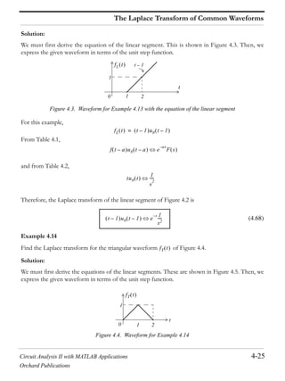
Solution:
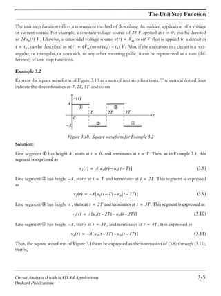
Using (5.6), we get
(5.9)
The residues are
(5.10)
and
(5.11)
Therefore, we express (5.9) as
(5.12)
and from Table 4.2 of Chapter 4
(5.13)
Then,
(5.14)
The residues and poles of a rational function of polynomials such as (5.8), can be found easily using
the MATLAB residue(a,b) function. For this example, we use the code
Ns = [3, 2]; Ds = [1, 3, 2]; [r, p, k] = residue(Ns, Ds)
and MATLAB returns the values
r =
4
-1
p =
-2
-1
k =
[]
F1 s
3s 2+
s
2
3s 2+ +
--------------------------
3s 2+
s 1+ s 2+
---------------------------------
r1
s 1+
----------------
r2
s 2+
----------------+= = =
r1 s 1+ F s
s 1–
lim 3s 2+
s 2+
----------------
s 1–=
1–= = =
r2 s 2+ F s
s 2–
lim
3s 2+
s 1+
----------------
s 2–=
4= = =
F1 s 3s 2+
s
2
3s 2+ +
-------------------------- 1–
s 1+
---------------- 4
s 2+
----------------+= =
e
at–
u0 t
1
s a+
-----------
F1 s 1–
s 1+
---------------- 4
s 2+
----------------+= e
t–
– 4e
2t–
+ u0 t f1 t=

164. Chapter 5 The Inverse Laplace Transformation
5-4 Circuit Analysis II with MATLAB Applications
Orchard Publications
For this MATLAB code, we defined Ns and Ds as two vectors that contain the numerator and
denominator coefficients of . When this code is executed, MATLAB displays the r and p vec-
tors that represent the residues and poles respectively. The first value of the vector r is associated
with the first value of the vector p, the second value of r is associated with the second value of p,
and so on.
The vector k is referred to as the direct term and it is always empty (has no value) whenever is
a proper rational function, that is, when the highest degree of the denominator is larger than that of
the numerator. For this example, we observe that the highest power of the denominator is ,
whereas the highest power of the numerator is and therefore the direct term is empty.
We can also use the MATLAB ilaplace(f) function to obtain the time domain function directly from
. This is done with the code that follows.
syms s t; Fs=(3*s+2)/(s^2+3*s+2); ft=ilaplace(Fs); pretty(ft)
When this code is executed, MATLAB displays the expression
4 exp(-2 t)- exp(-t)
Example 5.2
Use the partial fraction expansion method to simplify of (5.15) below, and find the time
domain function corresponding to .
(5.15)
Solution:
First, we use the MATLAB factor(s) symbolic function to express the denominator polynomial of
in factored form. For this example,
syms s; factor(s^3 + 12*s^2 + 44*s + 48)
ans =
(s+2)*(s+4)*(s+6)
Then,
(5.16)
The residues are
F s
F s
s2
s
F s
F2 s
f2 t F2 s
F2 s 3s
2
2s 5+ +
s
3
12s+
2
44s 48+ +
-------------------------------------------------=
F2 s
F2 s 3s
2
2s 5+ +
s
3
12s+
2
44s 48+ +
------------------------------------------------- 3s
2
2s 5+ +
s 2+ s 4+ s 6+
--------------------------------------------------
r1
s 2+
----------------
r2
s 4+
----------------
r3
s 6+
----------------+ += = =

165. Circuit Analysis II with MATLAB Applications 5-5
Orchard Publications
Partial Fraction Expansion
(5.17)
(5.18)
(5.19)
Then, by substitution into (5.16) we get
(5.20)
From Table 2.2 of Chapter 2
(5.21)
Then,
(5.22)
Check with MATLAB:
syms s t; Fs = (3*s^2 + 4*s + 5) / (s^3 + 12*s^2 + 44*s + 48); ft = ilaplace(Fs)
ft =
-37/4*exp(-4*t)+9/8*exp(-2*t)+89/8*exp(-6*t)
Case II: Complex Poles
Quite often, the poles of are complex*
, and since complex poles occur in complex conjugate
pairs, the number of complex poles is even. Thus, if is a complex root of , then, its complex
conjugate pole, denoted as , is also a root of . The partial fraction expansion method can
also be used in this case, but it may be necessary to manipulate the terms of the expansion in order to
express them in a recognizable form. The procedure is illustrated with the following example.
Example 5.3
Use the partial fraction expansion method to simplify of (5.23) below, and find the time
* A review of complex numbers is presented in Appendix B of Circuit Analysis I with MATLAB Applications.
r1
3s
2
2s 5+ +
s 4+ s 6+
---------------------------------
s 2–=
9
8
---= =
r2
3s
2
2s 5+ +
s 2+ s 6+
---------------------------------
s 4–=
37
4
------–= =
r3
3s
2
2s 5+ +
s 2+ s 4+
---------------------------------
s 6–=
89
8
------= =
F2 s
3s
2
2s 5+ +
s
3
12s+
2
44s 48+ +
-------------------------------------------------
9 8
s 2+
----------------
37 4–
s 4+
----------------
89 8
s 6+
----------------+ += =
e
at–
u0 t
1
s a+
-----------
F2 s 9 8
s 2+
---------------- 37 4–
s 4+
---------------- 89 8
s 6+
----------------+ +=
9
8
---e
2t– 37
4
------– e
4t– 89
8
------e
6t–
+ u0 t f2 t=
F s
pk D s
pk D s
F3 s

166. Chapter 5 The Inverse Laplace Transformation
5-6 Circuit Analysis II with MATLAB Applications
Orchard Publications
domain function corresponding to .
(5.23)
Solution:
Let us first express the denominator in factored form to identify the poles of using the MAT-
LAB factor(s) function. Then,
syms s; factor(s^3 + 5*s^2 + 12*s + 8)
ans =
(s+1)*(s^2+4*s+8)
The factor(s) function did not factor the quadratic term. We will use the roots(p) function.
p=[1 4 8]; roots_p=roots(p)
roots_p =
-2.0000 + 2.0000i
-2.0000 - 2.0000i
Then,
or
(5.24)
The residues are
(5.25)
(5.26)
(5.27)
By substitution into (5.24),
f3 t F3 s
F3 s s 3+
s
3
5s+
2
12s 8+ +
-------------------------------------------=
F3 s
F3 s
s 3+
s
3
5s+
2
12s 8+ +
-------------------------------------------
s 3+
s 1+ s 2 j2+ + s 2 j2–+
------------------------------------------------------------------------= =
F3 s
s 3+
s
3
5s+
2
12s 8+ +
-------------------------------------------
r1
s 1+
----------------
r2
s 2 j2+ +
---------------------------
r2
s 2 j– 2+
-------------------------+ += =
r1
s 3+
s
2
4s 8+ +
--------------------------
s 1–=
2
5
---= =
r2
s 3+
s 1+ s 2 j– 2+
------------------------------------------
s 2– j2–=
1 j2–
1– j2– j4–
------------------------------------ 1 j2–
8– j4+
------------------= = =
1 j2–
8– j4+
----------------------- 8– j4–
8– j4–
----------------------- 16– j12+
80
------------------------ 1
5
---– j3
20
------+= ==
r2
1
5
---–
j3
20
------+
1
5
---–
j3
20
------–= =

167. Circuit Analysis II with MATLAB Applications 5-7
Orchard Publications
Partial Fraction Expansion
(5.28)
The last two terms on the right side of (5.28), do not resemble any Laplace transform pair that we
derived in Chapter 2. Therefore, we will express them in a different form. We combine them into a
single term*, and now (5.28) is written as
(5.29)
For convenience, we denote the first term on the right side of (5.29) as , and the second as
. Then,
(5.30)
Next, for
(5.31)
and recalling that
(5.32)
we express as
(5.33)
* Here, we used MATLAB with simple(( 1/5 +3j/20)/(s+2+2j)+( 1/5 3j/20)/(s+2 2j)). The simple func-
tion, after several simplification tools that were displayed on the screen, returned (-2*s-1)/
(5*s^2+20*s+40)
F3 s 2 5
s 1+
---------------- 1 5– j3 20+
s 2 j2+ +
----------------------------------- 1 5– j3 20–
s 2 j– 2+
-----------------------------------+ +=
F3 s
2 5
s 1+
----------------
1
5
---
2s 1+
s
2
4s 8+ +
-------------------------------–=
F31 s
F32 s
F31 s
2 5
s 1+
----------------=
2
5
---e
t–
f31 t=
F32 s
F32 s
1
5
---–
2s 1+
s
2
4s 8+ +
-------------------------------=
e
at–
tu0tsin
s a+
2 2
+
-------------------------------
e
at–
tu0tcos
s a+
s a+
2 2
+
-------------------------------
F32 s
F32 s
2
5
---–
s 1
2
--- 3
2
--- 3
2
---–+ +
s 2+
2
2
2
+
--------------------------------- 2
5
---–
s 2+
s 2+
2
2
2
+
---------------------------------
3 2–
s 2+
2
2
2
+
---------------------------------+= =
2
5
---–
s 2+
s 2+
2
2
2
+
--------------------------------- 6 10
2
------------- 2
s 2+
2
2
2
+
---------------------------------+=
2
5
---–
s 2+
s 2+
2
2
2
+
--------------------------------- 3
10
------ 2
s 2+
2
2
2
+
---------------------------------+=

168. Chapter 5 The Inverse Laplace Transformation
5-8 Circuit Analysis II with MATLAB Applications
Orchard Publications
Addition of (5.30) with (5.33) yields
Check with MATLAB:
syms a s t w; % Define several symbolic variables
Fs=(s + 3)/(s^3 + 5*s^2 + 12*s + 8); ft=ilaplace(Fs)
ft =
2/5*exp(-t)-2/5*exp(-2*t)*cos(2*t)
+3/10*exp(-2*t)*sin(2*t)
Case III: Multiple (Repeated) Poles
In this case, has simple poles, but one of the poles, say , has a multiplicity . For this condi-
tion, we express it as
(5.34)
Denoting the residues corresponding to multiple pole as , the partial frac-
tion expansion of (5.34) is written as
(5.35)
For the simple poles , we proceed as before, that is, we find the residues as
(5.36)
The residues corresponding to the repeated poles, are found by multiplication of
both sides of (5.35) by . Then,
(5.37)
F3 s F31 s F32 s+
2 5
s 1+
---------------- 2
5
---–
s 2+
s 2+
2
2
2
+
---------------------------------
3
10
------
2
s 2+
2
2
2
+
---------------------------------+= =
2
5
---e
t– 2
5
---e
2t–
2t
3
10
------e
2t–
2tsin+cos– f3 t=
F s p1 m
F s
N s
s p1–
m
s p2– s pn 1–– s pn–
------------------------------------------------------------------------------------------=
m p1 r11 r12 r13 r1m
F s
r11
s p1–
m
---------------------
r12
s p1–
m 1–
----------------------------
r13
s p1–
m 2–
----------------------------
r1m
s p1–
------------------+ + + +=
+
r2
s p2–
------------------
r3
s p3–
------------------
rn
s pn–
------------------+ + +
p1 p2 pn
rk s pk– F s
s pk
lim s pk– F s
s pk=
= =
r11 r12 r13 r1m
s p–
m
s p1–
m
F s r11 s p1– r12 s p1–
2
r13 s p1–
m 1–
r1m+ + + +=
+ s p1–
m r2
s p2–
------------------
r3
s p3–
------------------
rn
s pn–
------------------+ + +

169. Circuit Analysis II with MATLAB Applications 5-9
Orchard Publications
Partial Fraction Expansion
Next, taking the limit as on both sides of (5.37), we get
or
(5.38)
and thus (5.38) yields the residue of the first repeated pole.
The residue for the second repeated pole , is found by differentiating (5.37) with respect to
and again, we let , that is,
(5.39)
In general, the residue can be found from
(5.40)
whose derivative of both sides is
(5.41)
or
(5.42)
Example 5.4
Use the partial fraction expansion method to simplify of (5.43) below, and find the time
domain function corresponding to .
(5.43)
Solution:
We observe that there is a pole of multiplicity 2 at , and thus in partial fraction expansion
form, is written as
s p1
s p1–
m
F s
s p1
lim r11 s p1– r12 s p1–
2
r13 s p1–
m 1–
r1m+ + +
s p1
lim+=
+ s p1–
m r2
s p2–
------------------
r3
s p3–
------------------
rn
s pn–
------------------+ + +
s p1
lim
r11 s p1–
m
F s
s p1
lim=
r12 p1 s
s p1
r12
d
ds
-----
s p1
lim s p1–
m
F s=
r1k
s p1–
m
F s r11 r12 s p1– r13 s p1–
2
+ + +=
m 1– th
k 1– !r1k
1
k 1– !
------------------
s p1
lim
d
k 1–
ds
k 1–
-------------- s p1–
m
F s=
r1k
1
k 1– !
------------------
s p1
lim
d
k 1–
ds
k 1–
-------------- s p1–
m
F s=
F4 s
f4 t F4 s
F4 s s 3+
s 2+ s 1+
2
-----------------------------------=
s 1–=
F4 s

170. Chapter 5 The Inverse Laplace Transformation
5-10 Circuit Analysis II with MATLAB Applications
Orchard Publications
(5.44)
The residues are
The value of the residue can also be found without differentiation as follows:
Substitution of the already known values of and into (5.44), and letting *
, we get
or
from which as before. Finally,
(5.45)
Check with MATLAB:
syms s t; Fs=(s+3)/((s+2)*(s+1)^2); ft=ilaplace(Fs)
ft = exp(-2*t)+2*t*exp(-t)-exp(-t)
We can use the following code to check the partial fraction expansion.
syms s
Ns = [1 3]; % Coefficients of the numerator N(s) of F(s)
expand((s + 1)^2); % Expands (s + 1)^2 to s^2 + 2*s + 1;
d1 = [1 2 1]; % Coefficients of (s + 1)^2 = s^2 + 2*s + 1 term in D(s)
d2 = [0 1 2]; % Coefficients of (s + 2) term in D(s)
* This is permissible since (5.44) is an identity.
F4 s
s 3+
s 2+ s 1+
2
-----------------------------------
r1
s 2+
----------------
r21
s 1+
2
------------------
r22
s 1+
----------------+ += =
r1
s 3+
s 1+
2
------------------
s 2–=
1= =
r21
s 3+
s 2+
-----------
s 1–=
2= =
r22
d
ds
-----
s 3+
s 2+
-----------
s 1–=
s 2+ s 3+–
s 2+
2
---------------------------------------
s 1–=
1–= = =
r22
r1 r21 s 0=
s 3+
s 1+
2
s 2+
-----------------------------------
s 0=
1
s 2+
----------------
s 0=
2
s 1+
2
------------------
s 0=
r22
s 1+
----------------
s 0=
+ +=
3
2
---
1
2
--- 2 r22+ +=
r22 1–=
F4 s s 3+
s 2+ s 1+
2
-----------------------------------= 1
s 2+
---------------- 2
s 1+
2
------------------ 1–
s 1+
----------------+ += e
2t–
2te
t–
e
t–
–+ f4 t=

171. Circuit Analysis II with MATLAB Applications 5-11
Orchard Publications
Partial Fraction Expansion
Ds=conv(d1,d2); % Multiplies polynomials d1 and d2 to express the
% denominator D(s) of F(s) as a polynomial
[r,p,k]=residue(Ns,Ds)
r =
1.0000
-1.0000
2.0000
p =
-2.0000
-1.0000
-1.0000
k =
[]
Example 5.5
Use the partial fraction expansion method to simplify of (5.46) below, and find the time
domain function corresponding to the given .
(5.46)
Solution:
We observe that there is a pole of multiplicity at , and a pole of multiplicity at .
Then, in partial fraction expansion form, is written as
(5.47)
The residues are
F5 s
f5 t F5 s
F5 s
s
2
3+ s 1+
s 1+
3
s 2+
2
--------------------------------------=
3 s 1–= 2 s 2–=
F5 s
F5 s
r11
s 1+
3
------------------
r12
s 1+
2
------------------
r13
s 1+
----------------
r21
s 2+
2
------------------
r22
s 2+
----------------+ + + +=
r11
s
2
3+ s 1+
s 2+
2
--------------------------
s 1–=
1–= =
r12
d
ds
----- s
2
3+ s 1+
s 2+
2
--------------------------
s 1–=
=
s 2+
2
2s 3+ 2 s 2+ s
2
3+ s 1+–
s 2+
4
----------------------------------------------------------------------------------------------
s 1–=
s 4+
s 2+
3
------------------
s 1–=
3= ==

172. Chapter 5 The Inverse Laplace Transformation
5-12 Circuit Analysis II with MATLAB Applications
Orchard Publications
Next, for the pole at ,
and
By substitution of the residues into (5.47), we get
(5.48)
We will check the values of these residues with the MATLAB code below.
syms s; % The function collect(s) below multiplies (s+1)^3 by (s+2)^2
% and we use it to express the denominator D(s) as a polynomial so that we can
% we can use the coefficients of the resulting polynomial with the residue function
Ds=collect(((s+1)^3)*((s+2)^2))
Ds =
s^5+7*s^4+19*s^3+25*s^2+16*s+4
Ns=[1 3 1]; Ds=[1 7 19 25 16 4]; [r,p,k]=residue(Ns,Ds)
r =
4.0000
1.0000
-4.0000
3.0000
-1.0000
r13
1
2!
-----
d
2
ds
2
--------
s
2
3+ s 1+
s 2+
2
--------------------------
s 1–=
1
2
---
d
ds
-----
d
ds
-----
s
2
3+ s 1+
s 2+
2
--------------------------
s 1–=
= =
1
2
--- d
ds
----- s 4+
s 2+
3
------------------
s 1–=
1
2
--- s 2+
3
3 s 2+
2
s 4+–
s 2+
6
----------------------------------------------------------------
s 1–=
==
1
2
---
s 2 3s– 12–+
s 2+
4
-----------------------------------
s 1–=
s– 5–
s 2+
4
------------------
s 1–=
4–= ==
s 2–=
r21
s
2
3+ s 1+
s 1+
3
--------------------------
s 2–=
1= =
r22
d
ds
-----
s
2
3+ s 1+
s 1+
3
--------------------------
s 2–=
s 1+
3
2s 3+ 3 s 1+
2
s
2
3+ s 1+–
s 1+
6
---------------------------------------------------------------------------------------------------
s 2–=
= =
s 1+ 2s 3+ 3 s
2
3+ s 1+–
s 1+
4
-----------------------------------------------------------------------------
s 2–=
s
2
– 4s–
s 1+
4
--------------------
s 2–=
4= ==
F5 s
1–
s 1+
3
------------------
3
s 1+
2
------------------
4–
s 1+
----------------
1
s 2+
2
------------------
4
s 2+
----------------+ + + +=

173. Circuit Analysis II with MATLAB Applications 5-13
Orchard Publications
Case for m n
p =
-2.0000
-2.0000
-1.0000
-1.0000
-1.0000
k =
[]
From Table 2.2 of Chapter 2
and with these, we derive from (5.48) as
(5.49)
We can verify (5.49) with MATLAB as follows:
syms s t; Fs= 1/((s+1)^3) + 3/((s+1)^2) 4/(s+1) + 1/((s+2)^2) + 4/(s+2);
ft=ilaplace(Fs)
ft = -1/2*t^2*exp(-t)+3*t*exp(-t)-4*exp(-t)
+t*exp(-2*t)+4*exp(-2*t)
5.3 Case for m n
Our discussion thus far, was based on the condition that is a proper rational function. However,
if is an improper rational function, that is, if , we must first divide the numerator by
the denominator to obtain an expression of the form
(5.50)
where is a proper rational function.
Example 5.6
Derive the Inverse Laplace transform of
(5.51)
e
at– 1
s a+
----------- te
at– 1
s a+
2
------------------ t
n 1–
e
at– n 1– !
s a+
n
------------------
f5 t
f5 t
1
2
---– t
2
e
t–
3te
t–
4e
t–
– te
2t–
4e
2t–
+ + +=
F s
F s m n N s
D s
F s k0 k1s k2s
2
km n– s
m n– N s
D s
-----------+ + + + +=
N s D s
f6 t
F6 s
s
2
2s 2+ +
s 1+
--------------------------=

174. Chapter 5 The Inverse Laplace Transformation
5-14 Circuit Analysis II with MATLAB Applications
Orchard Publications
Solution:
For this example, is an improper rational function. Therefore, we must express it in the form
of (5.50) before we use the partial fraction expansion method.
By long division, we get
Now, we recognize that
and
but
To answer that question, we recall that
and
where is the doublet of the delta function. Also, by the time differentiation property
Therefore, we have the new transform pair
(5.52)
and thus,
(5.53)
In general,
(5.54)
We verify (5.53) with MATLAB as follows:
Ns = [1 2 2]; Ds = [1 1]; [r, p, k] = residue(Ns, Ds)
r =
1
F6 s
F6 s s
2
2s 2+ +
s 1+
-------------------------- 1
s 1+
----------- 1 s+ += =
1
s 1+
----------- e
t–
1 t
s ?
u0' t t=
u0'' t ' t=
' t
u0'' t ' t= s
2
F s sf 0 f '– 0– s
2
F s s
2 1
s
--- s= = =
s ' t
F6 s s
2
2s 2+ +
s 1+
-------------------------- 1
s 1+
----------- 1 s+ += = e
t–
t ' t+ + f6 t=
d
n
dt
n
-------- t s
n

175. Circuit Analysis II with MATLAB Applications 5-15
Orchard Publications
Alternate Method of Partial Fraction Expansion
p =
-1
k =
1 1
Here, the direct terms k= [1 1] are the coefficients of and respectively.
5.4 Alternate Method of Partial Fraction Expansion
Partial fraction expansion can also be performed with the method of clearing the fractions, that is,
making the denominators of both sides the same, then equating the numerators. As before, we
assume that is a proper rational function. If not, we first perform a long division, and then work
with the quotient and the remainder as we did in Example 5.6. We also assume that the denominator
can be expressed as a product of real linear and quadratic factors. If these assumptions prevail,
we let be a linear factor of , and we assume that is the highest power of
that divides . Then, we can express as
(5.55)
Let be a quadratic factor of , and suppose that is the highest power
of this factor that divides . Now, we perform the following steps:
1. To this factor, we assign the sum of n partial fractions, that is,
2. We repeat step 1 for each of the distinct linear and quadratic factors of
3. We set the given equal to the sum of these partial fractions
4. We clear the resulting expression of fractions and arrange the terms in decreasing powers of
5. We equate the coefficients of corresponding powers of
6. We solve the resulting equations for the residues
Example 5.7
Express of (5.56) below as a sum of partial fractions using the method of clearing the fractions.
(5.56)
t ' t
F s
D s
s a– D s s a–
m
s a–
D s F s
F s
N s
D s
-----------
r1
s a–
-----------
r2
s a–
2
------------------
rm
s a–
m
-------------------+ += =
s
2
s+ + D s s
2
s+ +
n
D s
r1s k1+
s
2
s+ +
---------------------------
r2s k2+
s
2
s+ +
2
----------------------------------
rns kn+
s
2
s+ +
n
----------------------------------+ + +
D s
F s
s
s
F7 s
F7 s
2s– 4+
s
2
1+ s 1–
2
-------------------------------------=

176. Chapter 5 The Inverse Laplace Transformation
5-16 Circuit Analysis II with MATLAB Applications
Orchard Publications
Solution:
Using Steps 1 through 3 above, we get
(5.57)
With Step 4,
(5.58)
and with Step 5,
(5.59)
Relation (5.59) will be an identity is if each power of is the same on both sides of this relation.
Therefore, we equate like powers of and we get
(5.60)
Subtracting the second equation of (5.60) from the fourth, we get
or
(5.61)
By substitution of (5.61) into the first equation of (5.60), we get
or
(5.62)
Next, substitution of (5.61) and (5.62) into the third equation of (5.60) yields
or
(5.63)
Finally by substitution of (5.61), (5.62), and (5.63) into the fourth equation of (5.60), we get
F7 s 2s– 4+
s
2
1+ s 1–
2
-------------------------------------
r1s A+
s
2
1+
------------------
r21
s 1–
2
------------------
r22
s 1–
----------------+ += =
2s– 4+ r1s A+ s 1–
2
r21 s
2
1+ r22 s 1– s
2
1++ +=
2s– 4+ r1 r22+ s
3
2r1– A r22 r21+–+ s
2
+=
+ r1 2A– r22+ s A r22– r21++
s s
s
0 r1 r22+=
0 2r1– A r22 r21+–+=
2– r1 2A– r22+=
4 A r22– r21+=
4 2r1=
r1 2=
0 2 r22+=
r22 2–=
2– 2 2A– 2–=
A 1=

177. Circuit Analysis II with MATLAB Applications 5-17
Orchard Publications
Alternate Method of Partial Fraction Expansion
or
(5.64)
Substitution of these values into (5.57) yields
(5.65)
Example 5.8
Use partial fraction expansion to simplify of (5.66) below, and find the time domain function
corresponding to .
(5.66)
Solution:
This is the same transform as in Example 5.3, where we found that the denominator can be
expressed in factored form of a linear term and a quadratic. Thus, we write as
(5.67)
and using the method of clearing the fractions, we rewrite (5.67) as
(5.68)
As in Example 5.3,
(5.69)
Next, to compute and , we follow the procedure of this section and we get
(5.70)
Since is already known, we only need two equations in and . Equating the coefficient of
on the left side, which is zero, with the coefficients of on the right side of (5.70), we get
(5.71)
4 1 2 r21+ +=
r21 1=
F7 s
2s– 4+
s
2
1+ s 1–
2
-------------------------------------
2s 1+
s
2
1+
------------------
1
s 1–
2
------------------
2
s 1–
----------------–+= =
F8 s
f8 t F8 s
F8 s s 3+
s
3
5s+
2
12s 8+ +
-------------------------------------------=
D s
F8 s
F8 s
s 3+
s 1+ s
2
4s 8+ +
------------------------------------------------=
F8 s
s 3+
s 1+ s
2
4s 8+ +
------------------------------------------------
r1
s 1+
-----------
r2s r3+
s
2
4s 8+ +
--------------------------+= =
r1
s 3+
s
2
4s 8+ +
--------------------------
s 1–=
2
5
---= =
r2 r3
s 3+ r1 s
2
4s 8+ + r2s r3+ s 1++=
r1 r2 r3 s2
s2
0 r1= r2+

178. Chapter 5 The Inverse Laplace Transformation
5-18 Circuit Analysis II with MATLAB Applications
Orchard Publications
and since , then .
To obtain the third residue , we equate the constant terms of (5.70). Then, or
, or . Then, by substitution into (5.68), we get
(5.72)
as before.
The remaining steps are the same as in Example 5.3, and thus is the same as , that is,
5.5 Summary
The Inverse Laplace Transform Integral defined as
is difficult to evaluate because it requires contour integration using complex variables theory.
For most engineering problems we can refer to Tables of Properties, and Common Laplace trans-
form pairs to lookup the Inverse Laplace transform.
The partial fraction expansion method offers a convenient means of expressing Laplace trans-
forms in a recognizable form from which we can obtain the equivalent time-domain functions.
If the highest power of the numerator is less than the highest power of the denomina-
tor , i.e., , is said to be expressed as a proper rational function. If , is
an improper rational function.
The Laplace transform must be expressed as a proper rational function before applying the
partial fraction expansion. If is an improper rational function, that is, if , we must first
divide the numerator by the denominator to obtain an expression of the form
In a proper rational function, the roots of numerator are called the zeros of and the
roots of the denominator are called the poles of .
r1 2 5= r2 2 5–=
r3 3 8r1 r3+=
3 8 2 5 r3+= r3 1 5–=
F8 s
2 5
s 1+
----------------
1
5
---
2s 1+
s
2
4s 8+ +
-------------------------------–=
f8 t f3 t
f8 t f3 t
2
5
---e
t– 2
5
---e
2t–
2t
3
10
------e
2t–
2tsin+cos– u0 t==
L
1–
F s f t=
1
2 j
-------- F s
j–
j+
e
st
ds=
m N s n
D s m n F s m n F s
F s
F s m n
N s D s
F s k0 k1s k2s
2
km n– s
m n– N s
D s
-----------+ + + + +=
N s F s
D s F s

179. Circuit Analysis II with MATLAB Applications 5-19
Orchard Publications
Summary
The partial fraction expansion method can be applied whether the poles of are distinct, com-
plex conjugates, repeated, or a combination of these.
When is expressed as
are called the residues and are the poles of .
The residues and poles of a rational function of polynomials can be found easily using the MAT-
LAB residue(a,b) function. The direct term is always empty (has no value) whenever is a
proper rational function.
We can use the MATLAB factor(s) symbolic function to convert the denominator polynomial
form of into a factored form.
We can use the MATLAB collect(s) and expand(s) symbolic functions to convert the denomi-
nator factored form of into a polynomial form.
In this chapter we developed the new transform pair
and in general,
The method of clearing the fractions is an alternate method of partial fraction expansion.
F s
F s
F s
r1
s p1–
------------------
r2
s p2–
------------------
r3
s p3–
------------------
rn
s pn–
------------------+ + + +=
r1 r2 r3 rn p1 p2 p3 pn F s
F s
F2 s
F2 s
s ' t
d
n
dt
n
-------- t s
n

180. Chapter 5 The Inverse Laplace Transformation
5-20 Circuit Analysis II with MATLAB Applications
Orchard Publications
5.6 Exercises
1. Find the Inverse Laplace transform of the following:
a.
b.
c.
d.
e.
2. Find the Inverse Laplace transform of the following:
a.
b.
c.
d.
e.
3. Find the Inverse Laplace transform of the following:
a.
b. (See hint on next page)
4
s 3+
-----------
4
s 3+
2
------------------
4
s 3+
4
------------------
3s 4+
s 3+
5
------------------
s
2
6s 3+ +
s 3+
5
--------------------------
3s 4+
s
2
4s 85+ +
-----------------------------
4s 5+
s
2
5s 18.5+ +
---------------------------------
s
2
3s 2+ +
s
3
5s
2
10.5s 9+ + +
------------------------------------------------
s
2
16–
s
3
8s
2
24s 32+ + +
----------------------------------------------
s 1+
s
3
6s
2
11s 6+ + +
-------------------------------------------
3s 2+
s
2
25+
-----------------
5s
2
3+
s
2
4+
2
---------------------

181. Circuit Analysis II with MATLAB Applications 5-21
Orchard Publications
Exercises
Hint:
c.
d.
e.
4. Use the Initial Value Theorem to find given that the Laplace transform of is
Compare your answer with that of Exercise 3(c).
5. It is known that the Laplace transform has two distinct poles, one at , the other at
. It also has a single zero at , and we know that . Find and .
1
2
------- t t tcos+sin
s
2
s
2 2
+
2
------------------------
1
2
3
--------- tsin t tcos–
1
s
2 2
+
2
------------------------
2s 3+
s
2
4.25s 1+ +
---------------------------------
s
3
8s
2
24s 32+ + +
s
2
6s 8+ +
----------------------------------------------
e
2s– 3
2s 3+
3
----------------------
f 0 f t
2s 3+
s
2
4.25s 1+ +
---------------------------------
F s s 0=
s 1–= s 1= f t
t
lim 10= F s f t

182. Chapter 5 The Inverse Laplace Transformation
5-22 Circuit Analysis II with MATLAB Applications
Orchard Publications
5.7 Solutions to Exercises
1.
a.
b. c.
d.
e.
2.
a.
b.
c. Using the MATLAB factor(s) function we get:
syms s; factor(s^2+3*s+2), factor(s^3+5*s^2+10.5*s+9)
ans = (s+2)*(s+1)
ans = 1/2*(s+2)*(2*s^2+6*s+9)
4
s 3+
----------- 4e
3t– 4
s 3+
2
------------------ 4te
3t– 4
s 3+
4
------------------
4
3!
-----t
3
e
3t– 2
3
---t
3
e
3t–
=
3s 4+
s 3+
5
------------------
3 s 4 3 5 3 5 3–++
s 3+
5
----------------------------------------------------------- 3
s 3+ 5 3–
s 3+
5
-------------------------------- 3
1
s 3+
4
------------------ 5
1
s 3+
5
------------------–= = =
3
3!
-----t
3
e
3t– 5
4!
-----t
4
e
3t–
–
1
2
--- t
3
e
3t– 5
12
------t
4
e
3t–
–=
s
2
6s 3+ +
s 3+
5
-------------------------- s
2
6s 9 6–+ +
s 3+
5
----------------------------------- s 3+
2
s 3+
5
------------------ 6
s 3+
5
------------------– 1
s 3+
3
------------------ 6
1
s 3+
5
------------------–= = =
1
2!
-----t
2
e
3t– 6
4!
-----t
4
e
3t–
–
1
2
--- t
2
e
3t– 1
2
---t
4
e
3t–
–=
3s 4+
s
2
4s 85+ +
-----------------------------
3 s 4 3 2 3 2 3–++
s 2+
2
81+
----------------------------------------------------------- 3
s 2+ 2 3–
s 2+
2
9
2
+
-------------------------------- 3
s 2+
s 2+
2
9
2
+
------------------------------
1
9
---
2 9
s 2+
2
9
2
+
------------------------------–= = =
3
s 2+
s 2+
2
9
2
+
------------------------------
2
9
---
9
s 2+
2
9
2
+
------------------------------ 3e
2t–
9tcos
2
9
---e
2t–
9tsin––=
4s 5+
s
2
5s 18.5+ +
--------------------------------- 4s 5+
s
2
5s 6.25 12.25+ + +
----------------------------------------------------- 4s 5+
s 2.5+
2
3.5
2
+
--------------------------------------- 4
s 5 4+
s 2.5+
2
3.5
2
+
---------------------------------------= = =
4
s 10 4 10 4– 5 4+ +
s 2.5+
2
3.5
2
+
--------------------------------------------------------- 4
s 2.5+
s 2.5+
2
3.5
2
+
---------------------------------------
1
3.5
-------
5 3.5
s 2.5+
2
3.5
2
+
---------------------------------------–==
4
s 2.5+
s 2.5+
2
3.5
2
+
---------------------------------------
10
7
------
3.5
s 2.5+
2
3.5
2
+
---------------------------------------– 4e
2.5t–
3.5tcos
10
7
------e
2.5t–
3.5tsin–=

183. Circuit Analysis II with MATLAB Applications 5-23
Orchard Publications
Solutions to Exercises
Then,
d.
e.
3.
a.
b.
s
2
3s 2+ +
s
3
5s
2
10.5s 9+ + +
------------------------------------------------
s 1+ s 2+
s 2+ s
2
3s 4.5+ +
----------------------------------------------------
s 1+
s
2
3s 4.5+ +
-----------------------------------
s 1+
s
2
3s 2.25 2.25– 4.5+ + +
----------------------------------------------------------------= = =
s 1.5 1.5– 1+ +
s 1.5+
2
1.5
2
+
--------------------------------------------
s 1.5+
s 1.5+
2
1.5
2
+
--------------------------------------------
1
1.5
-------
0.5 1.5
s 1.5+
2
1.5
2
+
--------------------------------------------–==
s 1.5+
s 1.5+
2
1.5
2
+
--------------------------------------------
1
3
---
1.5
s 2.5+
2
3.5
2
+
---------------------------------------– e
1.5t–
1.5tcos
1
3
---e
1.5t–
1.5tsin–=
s
2
16–
s
3
8s
2
24s 32+ + +
----------------------------------------------
s 4+ s 4–
s 4+ s
2
4s 8+ +
------------------------------------------------
s 4–
s 2+
2
2
2
+
------------------------------
s 2 2– 4–+
s 2+
2
2
2
+
------------------------------= = =
s 2+
s 2+
2
2
2
+
------------------------------
1
2
---
6 2
s 2+
2
2
2
+
------------------------------–=
s 2+
s 2+
2
2
2
+
------------------------------ 3
2
s 2+
2
2
2
+
------------------------------– e
2t–
2tcos 3e
2t–
2tsin–=
s 1+
s
3
6s
2
11s 6+ + +
------------------------------------------- s 1+
s 1+ s 2+ s 3+
-------------------------------------------------- 1
s 2+ s 3+
---------------------------------= =
1
s 2+ s 3+
---------------------------------
r1
s 2+
-----------
r2
s 3+
----------- r1
1
s 3+
-----------
s 2–=
1 r2
1
s 2+
-----------
s 3–=
1–= == =+==
1
s 2+ s 3+
---------------------------------
1
s 2+
-----------
1
s 3+
-----------–= e
2t–
e
3t–
–=
3s 2+
s
2
25+
-----------------
3s
s
2
5
2
+
----------------
1
5
---
2 5
s
2
5
2
+
----------------+ 3
s
s
2
5
2
+
----------------
2
5
---
5
s
2
5
2
+
----------------+ 3 5t
2
5
--- 5tsin+cos= =
5s
2
3+
s
2
4+
2
---------------------
5s
2
s
2
2
2
+
2
-----------------------
3
s
2
2
2
+
2
-----------------------+ 5
1
2 2
------------ 2t 2t 2tcos+sin 3
1
2 8
------------ 2t 2t 2tcos–sin+=
5
4
---
3
16
------+ 2tsin
5
4
---
3
16
------– 2t 2tcos+
23
16
------ 2t
17
8
------t 2tcos+sin=

184. Chapter 5 The Inverse Laplace Transformation
5-24 Circuit Analysis II with MATLAB Applications
Orchard Publications
c.
d.
e.
4. The initial value theorem states that . Then,
The value is the same as in the time domain expression that we found in Exercise 3(c).
5. We are given that and . Then,
. Therefore,
, that is,
and we see that
2s 3+
s
2
4.25s 1+ +
--------------------------------- 2s 3+
s 4+ s 1 4+
----------------------------------------
r1
s 4+
-----------
r2
s 1 4+
------------------+= =
r1
2s 3+
s 1 4+
------------------
s 4–=
5–
15– 4
----------------
4
3
--- r2
2s 3+
s 4+
---------------
s 1 4–=
5 2
15 4
-------------= = 2
3
---== = =
4 3
s 4+
-----------
2 3
s 1 4+
------------------+
2
3
--- 2e
4t–
e
t 4–
+
s
3
8s
2
24s 32+ + +
s
2
6s 8+ +
----------------------------------------------
s 4+ s
2
4s 8+ +
s 2+ s 4+
------------------------------------------------
s
2
4s 8+ +
s 2+
-------------------------------= = and by long division
s
2
4s 8+ +
s 2+
-------------------------- s 2
4
s 2+
-----------+ += ' t 2 t 4e
2t–
+ +
e
2s– 3
2s 3+
3
---------------------- e
2s–
F s f t 2– u0 t 2–
F s
3
2s 3+
3
----------------------=
3 2
3
2s 3+
3
2
3
-------------------------------
3 8
2s 3+ 2
3
----------------------------------
3 8
s 3 2+
3
--------------------------
3
8
---
1
2!
-----t
2
e
3 2 t– 3
16
------t
2
e
3 2 t–
== = =
e
2s–
F s e
2s– 3
2s 3+
3
----------------------=
3
16
------ t 2–
2
e
3 2 t 2––
u0 t 2–
f t
t 0
lim sF s
s
lim=
f 0 s
2s 3+
s
2
4.25s 1+ +
---------------------------------
s
lim 2s
2
3s+
s
2
4.25s 1+ +
---------------------------------
s
lim= =
2s
2
s
2
3s s
2
+
s
2
s
2
4.25s s
2
1 s
2
+ +
------------------------------------------------------------
s
lim 2 3 s+
1 4.25 s 1 s
2
+ +
--------------------------------------------
s
lim 2= ==
f 0 2=
F s
A s 1–
s s 1+
--------------------= f t
t
lim sF s
s 0
lim 10= =
s
A s 1–
s s 1+
--------------------
s 0
lim A s 1–
s 1+
----------------
s 0
lim A– 10= = =
F s 10– s 1–
s s 1+
-------------------------
r1
s
----
r2
s 1+
-----------+ 10
s
------ 20
s 1+
-----------–= = = 10 20e
t–
– u0 t
f t 10 20e
t–
– u0 t= f t
t
lim 10=

185. Circuit Analysis II with MATLAB Applications 6-1
Orchard Publications
Chapter 6
Circuit Analysis with Laplace Transforms
his chapter presents applications of the Laplace transform. Several examples are given to illus-
trate how the Laplace transformation is applied to circuit analysis. Complex impedance, com-
plex admittance, and transfer functions are also defined.
6.1 Circuit Transformation from Time to Complex Frequency
In this section we will derive the voltage-current relationships for the three elementary circuit
devices, i.e., resistors, inductors, and capacitors in the complex frequency domain.
a. Resistor
The time and complex frequency domains for purely resistive circuits are shown in Figure 6.1.
Figure 6.1. Resistive circuit in time domain and complex frequency domain
b. Inductor
The time and complex frequency domains for purely inductive circuits is shown in Figure 6.2.
Figure 6.2. Inductive circuit in time domain and complex frequency domain
c. Capacitor
The time and complex frequency domains for purely capacitive circuits is shown in Figure 6.3.
T
vR t RiR t=
iR t
vR t
R
------------=R
+
Time Domain
vR t
iR t
R
+
Complex Frequency Domain
VR s IR s
VR s RIR s=
IR s
VR s
R
--------------=
+
Time Domain
LvL t iL t
vL t L
diL
dt
-------=
iL t
1
L
--- vL td
–
t
=
+
Complex Frequency Domain
+
sL
LiL 0
VL s
IL s
VL s sLIL s LiL 0–=
IL s
VL s
Ls
-------------
iL 0
s
--------------+=

186. Chapter 6 Circuit Analysis with Laplace Transforms
6-2 Circuit Analysis II with MATLAB Applications
Orchard Publications
Figure 6.3. Capacitive circuit in time domain and complex frequency domain
Note:
In the complex frequency domain, the terms and are called complex inductive impedance,
and complex capacitive impedance respectively. Likewise, the terms and and are called com-
plex capacitive admittance and complex inductive admittance respectively.
Example 6.1
Use the Laplace transform method to find the voltage across the capacitor for the circuit of
Figure 6.4, given that .
Figure 6.4. Circuit for Example 6.1
Solution:
We apply KCL at node as shown in Figure 6.5.
Figure 6.5. Application of KCL for the circuit of Example 6.1
Then,
or
+
Time Domain
+C
vC t
iC t
iC t C
dvC
dt
---------=
vC t
1
C
---- iC td
–
t
=
+
Complex Frequency Domain
+
+
VC s
vC 0
s
----------------
IC s
1
sC
------ IC s sCVC s CvC 0–=
VC s
IC s
sC
------------
vC 0
s
----------------+=
sL 1 sC
sC 1 sL
vC t
vC 0 6 V=
R
C ++
V 1 F12u0 t
vS
vC t
A
R
C ++
V 1 F12u0 t
vS
vC t
AiR
iC
iR iC+ 0=

187. Circuit Analysis II with MATLAB Applications 6-3
Orchard Publications
Circuit Transformation from Time to Complex Frequency
or
(6.1)
The Laplace transform of (6.1) is
or
or
By partial fraction expansion,
Therefore,
Example 6.2
Use the Laplace transform method to find the current through the capacitor for the circuit of
Figure 6.6, given that .
Figure 6.6. Circuit for Example 6.2
vC t 12u0 t–
1
------------------------------------- 1
dvC
dt
---------+ 0=
dvC
dt
--------- vC t+ 12u0 t=
sVC s vC 0 VC s+– 12
s
------=
s 1+ VC s
12
s
------ 6+=
VC s 6s 12+
s s 1+
-------------------=
VC s
6s 12+
s s 1+
-------------------
r1
s
----
r2
s 1+
----------------+= =
r1
6s 12+
s 1+
------------------
s 0=
12= =
r2
6s 12+
s
------------------
s 1–=
6–= =
VC s
12
s
------
6
s 1+
-----------–= 12 6e
t–
– 12 6e
t–
– u0 t vC t= =
iC t
vC 0 6 V=
C ++
V 1 F12u0 t
vS
vC t
iC t

188. Chapter 6 Circuit Analysis with Laplace Transforms
6-4 Circuit Analysis II with MATLAB Applications
Orchard Publications
Solution:
This is the same circuit as in Example 6.1. We apply KVL for the loop shown in Figure 6.7.
Figure 6.7. Application of KVL for the circuit of Example 6.2
and with and , we get
(6.2)
Next, taking the Laplace transform of both sides of (6.2), we get
or
Check: From Example 6.1,
Then,
(6.3)
The presence of the delta function in (6.3) is a result of the unit step that is applied at .
R
C ++
V 1 F12u0 t
vS
vC t
iC t
RiC t
1
C
---- iC t td
–
t
+ 12u0 t=
R 1= C 1=
iC t iC t td
–
t
+ 12u0 t=
IC s
IC s
s
------------
vC 0
s
----------------+ +
12
s
------=
1
1
s
---+ IC s
12
s
------
6
s
---–
6
s
---= =
s 1+
s
----------- IC s
6
s
---=
IC s
6
s 1+
-----------= iC t 6e
t–
u0 t=
vC t 12 6e
t–
– u0 t=
iC t C
dvC
dt
---------
dvC
dt
---------
td
d
12 6e
t–
– u0 t 6e
t–
u0 t 6 t+= = = =
t 0=

189. Circuit Analysis II with MATLAB Applications 6-5
Orchard Publications
Circuit Transformation from Time to Complex Frequency
Example 6.3
In the circuit of Figure 6.8, switch closes at , while at the same time, switch opens. Use
the Laplace transform method to find for .
Figure 6.8. Circuit for Example 6.3
Solution:
Since the circuit contains a capacitor and an inductor, we must consider two initial conditions One
is given as . The other initial condition is obtained by observing that there is an initial
current of in inductor ; this is provided by the current source just before switch
opens. Therefore, our second initial condition is .
For , we transform the circuit of Figure 6.8 into its s-domain*
equivalent shown in Figure 6.9.
Figure 6.9. Transformed circuit of Example 6.3
In Figure 6.9 the current in has been replaced by a voltage source of . This is found from the
relation
(6.4)
* Henceforth, for convenience, we will refer the time domain as t-domain and the complex frequency domain as s-
domain
S1 t 0= S2
vout t t 0
+
C +
1
2 A
1 F
2
0.5 H
0.5 H
vC 0 3 V=
t 0=
t 0=
is t
vout t
iL1 t
L2
R1
R2
L1
S1
S2
vC 0 3 V=
2 A L1 2 A S2
iL1 0 2 A=
t 0
+
+
1
2 0.5s
0.5s
+
1/s
3/s
1 V
1
Vout s
L1 1 V
L1iL1 0
1
2
--- 2 1 V= =

190. Chapter 6 Circuit Analysis with Laplace Transforms
6-6 Circuit Analysis II with MATLAB Applications
Orchard Publications
The polarity of this voltage source is as shown in Figure 6.9 so that it is consistent with the direction
of the current in the circuit of Figure 6.8 just before switch opens.
The initial capacitor voltage is replaced by a voltage source equal to .
Applying KCL at node , we get
(6.5)
and after simplification
(6.6)
We will use MATLAB to factor the denominator of (6.6) into a linear and a quadratic factor.
p=[1 8 10 4]; r=roots(p) % Find the roots of D(s)
r =
-6.5708
-0.7146 + 0.3132i
-0.7146 - 0.3132i
y=expand((s + 0.7146 0.3132j)*(s + 0.7146 + 0.3132j))% Find quadratic form
y =
s^2+3573/2500*s+3043737/5000000
3573/2500 % Find coefficient of s
ans =
1.4292
3043737/5000000 % Find constant term
ans =
0.6087
Therefore,
(6.7)
Now, we perform partial fraction expansion.
(6.8)
iL1 t S2
3 s
Vout s 1– 3 s–
1 s 2 s 2+ +
------------------------------------------
Vout s
1
-----------------
Vout s
s 2
-----------------+ + 0=
Vout s
2s s 3+
s
3
8s
2
10s 4+ + +
-------------------------------------------=
D s
Vout s 2s s 3+
s
3
8s
2
10s 4+ + +
------------------------------------------- 2s s 3+
s 6.57+ s
2
1.43s 0.61+ +
----------------------------------------------------------------------= =
Vout s 2s s 3+
s 6.57+ s
2
1.43s 0.61+ +
----------------------------------------------------------------------
r1
s 6.57+
-------------------
r2 s r3+
s
2
1.43s 0.61+ +
-----------------------------------------+==

191. Circuit Analysis II with MATLAB Applications 6-7
Orchard Publications
Circuit Transformation from Time to Complex Frequency
(6.9)
The residues and are found from the equality
(6.10)
Equating constant terms of (6.10), we get
and by substitution of the known value of from (6.9), we get
Similarly, equating coefficients of , we get
and using the known value of , we get
(6.11)
By substitution into (6.8),
*
or
(6.12)
Taking the Inverse Laplace of (6.12), we get
* We perform these steps to express the term in a form that resembles the transform pairs
and . The remaining steps are carried out in
(6.12).
r1
2s s 3+
s
2
1.43s 0.61+ +
-----------------------------------------
s 6.57–=
1.36= =
r2 r3
2s s 3+ r1 s
2
1.43s 0.61+ + r2 s r3+ s 6.57++=
0 0.61r1 6.57r3+=
r1
r3 0.12–=
s2
2 r1 r2+=
r1
r2 0.64=
Vout s
1.36
s 6.57+
-------------------
0.64s 0.12–
s
2
1.43s 0.61+ +
-----------------------------------------+
1.36
s 6.57+
-------------------
0.64s 0.46 0.58–+
s
2
1.43s 0.51 0.1+ + +
-------------------------------------------------------+= =
0.64s 0.12–
s
2
1.43s 0.61+ +
-----------------------------------------
e
at–
tu0 tcos
s a+
s a+
2 2
+
-------------------------------- e
at–
tu0 tsin
s a+
2 2
+
--------------------------------
Vout s
1.36
s 6.57+
------------------- 0.64
s 0.715 0.91–+
s 0.715+
2
0.316
2
+
--------------------------------------------------------+=
1.36
s 6.57+
-------------------
0.64 s 0.715+
s 0.715+
2
0.316
2
+
--------------------------------------------------------
0.58
s 0.715+
2
0.316
2
+
--------------------------------------------------------–+=
1.36
s 6.57+
-------------------
0.64 s 0.715+
s 0.715+
2
0.316
2
+
--------------------------------------------------------
1.84 0.316
s 0.715+
2
0.316
2
+
--------------------------------------------------------–+=

192. Chapter 6 Circuit Analysis with Laplace Transforms
6-8 Circuit Analysis II with MATLAB Applications
Orchard Publications
(6.13)
6.2 Complex Impedance Z(s)
Consider the -domain series circuit of Figure 6.10, where the initial conditions are assumed to
be zero.
Figure 6.10. Series RLC circuit in s-domain
For this circuit, the sum represents the total opposition to current flow. Then,
(6.14)
and defining the ratio as , we get
(6.15)
and thus, the -domain current can be found from
(6.16)
where
(6.17)
We recall that . Therefore, is a complex quantity, and it is referred to as the complex
input impedance of an -domain series circuit. In other words, is the ratio of the voltage
excitation to the current response under zero state (zero initial conditions).
vout t 1.36e
6.57t–
0.64e
0.715t–
0.316tcos 1.84e
0.715t–
0.316tsin–+ u0 t=
s RLC
+
R
+
VS s
I s
sL
1
sC
------
Vout s
R sL
1
sC
------+ +
I s
VS s
R sL 1 sC+ +
------------------------------------=
Vs s I s Z s
Z s
VS s
I s
------------- R sL 1
sC
------+ +=
s I s
I s
VS s
Z s
-------------=
Z s R sL
1
sC
------+ +=
s j+= Z s
s RLC Z s
Vs s I s

193. Circuit Analysis II with MATLAB Applications 6-9
Orchard Publications
Complex Impedance Z(s)
Example 6.4
Find for the circuit of Figure 6.11. All values are in (ohms).
Figure 6.11. Circuit for Example 6.4
Solution:
First Method:
We will first find , and we will compute from (6.15). We assign the voltage at node
as shown in Figure 6.12.
Figure 6.12. Circuit for finding in Example 6.4
By nodal analysis,
The current is now found as
and thus,
(6.18)
Z s
+
1
VS s
1 s
s s
I s Z s VA s
A
+
1
VS s
1 s
s s
I s
VA s
A
I s
VA s VS s–
1
---------------------------------
VA s
s
--------------
VA s
s 1 s+
------------------+ + 0=
1
1
s
---
1
s 1 s+
------------------+ + VA s VS s=
VA s
s
3
1+
s
3
2s
2
s 1+ + +
------------------------------------- VS s=
I s
I s
VS s VA s–
1
--------------------------------- 1
s
3
1+
s
3
2s
2
s 1+ + +
-------------------------------------– VS s
2s
2
1+
s
3
2s
2
s 1+ + +
------------------------------------- VS s= = =
Z s
VS s
I s
-------------
s
3
2s
2
s 1+ + +
2s
2
1+
-------------------------------------= =

194. Chapter 6 Circuit Analysis with Laplace Transforms
6-10 Circuit Analysis II with MATLAB Applications
Orchard Publications
Second Method:
We can also compute by successive combinations of series and parallel impedances, as it is
done with series and parallel resistances. For this example, we denote the network devices as
and shown in Figure 6.13.
Figure 6.13. Computation of the impedance of Example 6.4 by series parallel combinations
To find the equivalent impedance , looking to the right of terminals and , we start on the
right side of the network and we proceed to the left combining impedances as we combine resis-
tances. Then,
(6.19)
We observe that (6.19) is the same as (6.18).
6.3 Complex Admittance Y(s)
Consider the -domain parallel circuit of Figure 6.14 where the initial conditions are zero.
Figure 6.14. Parallel GLC circuit in s-domain
For this circuit,
Defining the ratio as , we get
Z s
Z1 Z2 Z3 Z4
1 1 s
s sZ s
Z1
Z2
Z3
Z4
a
b
Z s a b
Z s Z3 Z4+ || Z2 Z1+=
Z s
s s 1 s+
s s 1 s+ +
-------------------------- 1+
s
2
1+
2s
2
1+ s
---------------------------- 1+
s
3
s+
2s
2
1+
----------------- 1+
s
3
2s
2
s 1+ + +
2s
2
1+
-------------------------------------= = = =
s GLC
G
+
IS s
V s
1
sL
------
sC
GV s
1
sL
------V s sCV s+ + I s=
G
1
sL
------ sC+ + V s I s=
IS s V s Y s

195. Circuit Analysis II with MATLAB Applications 6-11
Orchard Publications
Complex Admittance Y(s)
(6.20)
and thus the -domain voltage can be found from
(6.21)
where
(6.22)
We recall that . Therefore, is a complex quantity, and it is referred to as the complex
input admittance of an -domain parallel circuit. In other words, is the ratio of the cur-
rent excitation to the voltage response under zero state (zero initial conditions).
Example 6.5
Compute and for the circuit of Figure 6.15. All values are in (ohms). Verify your
answers with MATLAB.
Figure 6.15. Circuit for Example 6.5
Solution:
It is convenient to represent the given circuit as shown in Figure 6.16.
Figure 6.16. Simplified circuit for Example 6.5
Y s
I s
V s
----------- G 1
sL
------ sC+ + 1
Z s
----------= =
s V s
V s
IS s
Y s
-----------=
Y s G
1
sL
------ sC+ +=
s j+= Y s
s GLC Y s
IS s V s
Z s Y s
Z s
Y s
13s
8 s
5s
16 s
10 20
Z3
Z2
Z1
Z s Y s

196. Chapter 6 Circuit Analysis with Laplace Transforms
6-12 Circuit Analysis II with MATLAB Applications
Orchard Publications
where
Then,
Check with MATLAB:
syms s; z1 = 13*s + 8/s; z2 = 5*s + 10; z3 = 20 + 16/s; z = z1 + z2 * z3 / (z2+z3)
z =
13*s+8/s+(5*s+10)*(20+16/s)/(5*s+30+16/s)
z10 = simplify(z)
z10 =
(65*s^4+490*s^3+528*s^2+400*s+128)/s/(5*s^2+30*s+16)
pretty(z10)
4 3 2
65 s + 490 s + 528 s + 400 s + 128
-------------------------------------
2
s (5 s + 30 s + 16)
The complex input admittance is found by taking the reciprocal of , that is,
(6.23)
Z1 13s
8
s
---+
13s
2
8+
s
--------------------= =
Z2 10 5s+=
Z3 20
16
s
------+
4 5s 4+
s
-----------------------= =
Z s Z1
Z2Z3
Z2 Z3+
-----------------+
13s
2
8+
s
--------------------
10 5s+
4 5s 4+
s
-----------------------
10 5s+ 4 5s 4+
s
-----------------------+
----------------------------------------------------+= =
13s
2
8+
s
--------------------
10 5s+
4 5s 4+
s
-----------------------
5s
2
10s 4 5s 4++ +
s
----------------------------------------------------
-----------------------------------------------------
13s
2
8+
s
--------------------
20 5s
2
14s 8+ +
5s
2
30s 16+ +
-------------------------------------------+=+=
65s
4
490s
3
528s
2
400s 128+ + + +
s 5s
2
30s 16+ +
-------------------------------------------------------------------------------------=
Y s Z s
Y s
1
Z s
----------
s 5s
2
30s 16+ +
65s
4
490s
3
528s
2
400s 128+ + + +
-------------------------------------------------------------------------------------= =

197. Circuit Analysis II with MATLAB Applications 6-13
Orchard Publications
Transfer Functions
6.4 Transfer Functions
In an -domain circuit, the ratio of the output voltage to the input voltage under
zero state conditions, is of great interest in network analysis. This ratio is referred to as the voltage
transfer function and it is denoted as , that is,
(6.24)
Similarly, the ratio of the output current to the input current under zero state condi-
tions, is called the current transfer function denoted as , that is,
(6.25)
The current transfer function of (6.25) is rarely used; therefore, from now on, the transfer function
will have the meaning of the voltage transfer function, i.e.,
(6.26)
Example 6.6
Derive an expression for the transfer function for the circuit of Figure 6.17, where repre-
sents the internal resistance of the applied (source) voltage , and represents the resistance of
the load that consists of , , and .
Figure 6.17. Circuit for Example 6.6
Solution:
No initial conditions are given, and even if they were, we would disregard them since the transfer
function was defined as the ratio of the output voltage to the input voltage under
s Vout s Vin s
Gv s
Gv s
Vout s
Vin s
-----------------
Iout s Iin s
Gi s
Gi s
Iout s
Iin s
----------------
G s
Vout s
Vin s
-----------------
G s Rg
VS RL
RL L C
+
+
Rg
RL
L
C
vout
vg
Vout s Vin s

198. Chapter 6 Circuit Analysis with Laplace Transforms
6-14 Circuit Analysis II with MATLAB Applications
Orchard Publications
zero initial conditions. The -domain circuit is shown in Figure 6.18.
Figure 6.18. The s-domain circuit for Example 6.6
The transfer function is readily found by application of the voltage division expression of the
-domain circuit of Figure 6.18, i.e.,
Then,
(6.27)
Example 6.7
Compute the transfer function for the circuit of Figure 6.19 in terms of the circuit constants
Then, replace the complex variable with , and the circuit constants with
their numerical values and plot the magnitude versus radian frequency .
Figure 6.19. Circuit for Example 6.7
Solution:
The -domain equivalent circuit is shown in Figure 6.20.
s
+
+
Vin s
Rg
RL
sL
1
sC
------
Vout s
G s
s
Vout s
RL sL 1 sC+ +
Rg RL sL 1 sC+ + +
---------------------------------------------------Vin s=
G s
Vout s
Vin s
-----------------=
RL Ls 1 sC+ +
Rg RL Ls 1 sC+ + +
---------------------------------------------------=
G s
R1 R2 R3 C1 and C2 s j
G s Vout s Vin s=
vin vout
40 K
200 K 50K
25 nF
10 nF
R2
R1
C2
C1
R3
s

199. Circuit Analysis II with MATLAB Applications 6-15
Orchard Publications
Transfer Functions
Figure 6.20. The s-domain circuit for Example 6.7
Next, we write nodal equations at nodes 1 and 2.
At node 1,
(6.28)
At node 2,
(6.29)
Since (virtual ground), we express (6.29) as
(6.30)
and by substitution of (6.30) into (6.28), rearranging, and collecting like terms, we get:
or
(6.31)
By substitution of with and the given values for resistors and capacitors, we get
or
R2
1/sC1
R3
R1
1/sC2
Vin (s) Vout (s)
1 2
V1 s V2 s
V1 s Vin s–
R1
----------------------------------
V1
1 sC1
---------------
V1 s Vout s–
R2
-------------------------------------
V1 s V2 s–
R3
--------------------------------+ + + 0=
V2 s V1 s–
R3
--------------------------------
Vout s
1 sC2
------------------=
V2 s 0=
V1 s sR– 3C2 Vout s=
1
R1
----- 1
R2
----- 1
R3
----- sC1+ + + sR– 3C2
1
R2
-----– Vout s
1
R1
-----Vin s=
G s
Vout s
Vin s
------------------= 1–
R1
1
R1
----- 1
R2
----- 1
R3
----- sC1+ + + sR3C2
1
R2
-----+
-----------------------------------------------------------------------------------------------------=
s j
G j 1–
2 10
5 1
20 10
3
------------------- j2.5 10
8–
+ j5 10
4
10
8– 1
4 10
4
----------------+
--------------------------------------------------------------------------------------------------------------------------------------------------------------=

200. Chapter 6 Circuit Analysis with Laplace Transforms
6-16 Circuit Analysis II with MATLAB Applications
Orchard Publications
(6.32)
We use MATLAB to plot the magnitude of (6.32) on a semilog scale with the following code:
w=1:10:10000; Gs= 1./(2.5.*10.^( 6).*w.^2 5.*j.*10.^( 3).*w+5);
semilogx(w,abs(Gs)); grid; hold on
xlabel('Radian Frequency w'); ylabel('|Vout/Vin|');
title('Magnitude Vout/Vin vs. Radian Frequency')
The plot is shown in Figure 6.21. We observe that the given op amp circuit is a second order low-
pass filter whose cutoff frequency ( ) occurs at about .
Figure 6.21. versus for the circuit of Example 6.7
G j
Vout j
Vin j
---------------------= 1–
2.5 10
6– 2
j5 10
3–
5+–
------------------------------------------------------------------------=
3 dB– 700 r s
G j

201. Circuit Analysis II with MATLAB Applications 6-17
Orchard Publications
Summary
6.5 Summary
The Laplace transformation provides a convenient method of analyzing electric circuits since
integrodifferential equations in the -domain are transformed to algebraic equations in the -
domain.
In the -domain the terms and are called complex inductive impedance, and complex
capacitive impedance respectively. Likewise, the terms and and are called complex
capacitive admittance and complex inductive admittance respectively.
The expression
is a complex quantity, and it is referred to as the complex input impedance of an -domain
series circuit.
In the -domain the current can be found from
The expression
is a complex quantity, and it is referred to as the complex input admittance of an -domain
parallel circuit.
In the -domain the voltage can be found from
In an -domain circuit, the ratio of the output voltage to the input voltage under
zero state conditions is referred to as the voltage transfer function and it is denoted as , that
is,
t s
s sL 1 sC
sC 1 sL
Z s R sL
1
sC
------+ +=
s RLC
s I s
I s
VS s
Z s
-------------=
Y s G 1
sL
------ sC+ +=
s GLC
s V s
V s
IS s
Y s
-----------=
s Vout s Vin s
G s
G s
Vout s
Vin s
-----------------

202. Chapter 6 Circuit Analysis with Laplace Transforms
6-18 Circuit Analysis II with MATLAB Applications
Orchard Publications
6.6 Exercises
1. In the circuit of Figure 6.22, switch has been closed for a long time, and opens at . Use
the Laplace transform method to compute for .
Figure 6.22. Circuit for Exercise 1
2. In the circuit of Figure 6.23, switch has been closed for a long time, and opens at . Use
the Laplace transform method to compute for .
Figure 6.23. Circuit for Exercise 2
3. Use mesh analysis and the Laplace transform method, to compute and for the circuit
of Figure 6.24, given that and .
Figure 6.24. Circuit for Exercise 3
S t 0=
iL t t 0
1 mH
S
t 0=
iL t
+
L
32 V
10
20
R1
R2
S t 0=
vc t t 0
S
t 0=
+
72 V
6 K
C +60 K
30 K 20 K
10 K
40
9
------ F
vC t
R1
R2
R3
R4
R5
i1 t i2 t
iL(0 0= vC(0 0=
+
C +
1
3
1 F
i1 t +
1 H
v1 t u0 t=
v2 t 2u0 t=
2 H
i2 t
L1
R1
R2
L2

203. Circuit Analysis II with MATLAB Applications 6-19
Orchard Publications
Exercises
4. For the -domain circuit of Figure 6.25,
a. compute the admittance
b. compute the -domain value of when , and all initial conditions are zero.
Figure 6.25. Circuit for Exercise 4
5. Derive the transfer functions for the networks (a) and (b) of Figure 6.26.
Figure 6.26. Networks for Exercise 5
6. Derive the transfer functions for the networks (a) and (b) of Figure 6.27.
Figure 6.27. Networks for Exercise 6
7. Derive the transfer functions for the networks (a) and (b) of Figure 6.28.
s
Y s I1 s V1 s=
t i1 t v1 t u0 t=
R1
R2+
1
+
R3
1
31 s
V1 s
VC sI1 s
+
V2 s 2VC s=2R4
R
C
++
Vin s Vout s R
L
+
Vin s
+
Vout s
(a) (b)
R
C
++
Vin s Vout s
R
L
+
Vin s
+
Vout s
(a) (b)

204. Chapter 6 Circuit Analysis with Laplace Transforms
6-20 Circuit Analysis II with MATLAB Applications
Orchard Publications
Figure 6.28. Networks for Exercise 7
8. Derive the transfer function for the networks (a) and (b) of Figure 6.29.
Figure 6.29. Networks for Exercise 8
9. Derive the transfer function for the network of Figure 6.30. Using MATLAB, plot versus
frequency in Hertz, on a semilog scale.
Figure 6.30. Network for Exercise 9
R
C ++
Vin s Vout s
R
L
+
Vin s
+
Vout s
(a) (b)
L
R2R1
C
R1
Vin s
Vout s
R2
C
Vin s Vout s
(a) (b)
G s
R1 R2
R3
C1
C2
Vout s
Vin s
R4 R1 = 11.3 k
R2 = 22.6 k
R3=R4 = 68.1 k
C1=C2 = 0.01 F

205. Circuit Analysis II with MATLAB Applications 6-21
Orchard Publications
Solutions to Exercises
6.7 Solutions to Exercises
1. At the -domain circuit is as shown below and the resistor is shorted out by the
inductor.
Then,
and thus the initial condition has been established as
For all the -domain and -domain circuits are as shown below.
From the -domain circuit above we get
2. At the -domain circuit is as shown below.
Then,
t 0= t 20
1 mH
S
iL t
+
L
32 V
10
20
iL t
t 0
-
=
32
10
------ 3.2 A= =
iL 0 3.2 A=
t 0 t s
1 mH
iL 0 3.2 A=
+
20
LiL 0 3.2 10
3–
V=
20
IL s
10
3–
s
s
IL s
3.2 10
3–
20 10
3–
s+
-------------------------
3.2
s 20000+
-----------------------= = 3.2e
20000t–
u0 t iL t=
t 0= t
+
72 V
6 K +
60 K
30 K 20 K
10 KvC t
iT t
i2 t

206. Chapter 6 Circuit Analysis with Laplace Transforms
6-22 Circuit Analysis II with MATLAB Applications
Orchard Publications
and
Therefore, the initial condition is
For all the -domain circuit is as shown below.
Then,
3. The -domain circuit is shown below where , , and
iT 0
72 V
6 K 60 K 60 K+
------------------------------------------------------------
72 V
6 K 30 K+
-------------------------------------
72 V
36 K
-----------------= = 2 mA= =
i2 0
1
2
---iT 0 1 mA= =
vC 0 20 K 10 K+ i2 0 30 K 1 mA 30 V= = =
t 0 s
+
60 K
30 K 20 K
10 K
1
40 9 10
6–
s
----------------------------------
30 s
+
22.5 K
9 10
6
40s
-------------------
30 s
60 K 30 K+ 20 K 10 K+ 22.5 K=
VC s
VR
VR VC s=
+
VC s VR
22.5 10
3
9 10
6
40s 22.5 10
3
+
-------------------------------------------------------------
30
s
------ 30 22.5 10
3
9 10
6
40 22.5 10
3
s+
-------------------------------------------------------------= = =
30 22.5 10
3
22.5 10
3
9 10
6
40 22.5 10
3
s+
----------------------------------------------------------------------------
30
9 10
6
90 10
4
s+
---------------------------------------------------
30
10 s+
--------------= ==
VC s
30
s 10+
--------------= 30e
10t–
u0 t V vC t=
s z1 2s= z2 1 1 s+= z3 s 3+=
+
+
I1 s +
I2 s
2s
1 s
1 s
1 s
2 s
3
z1
z3
z2

207. Circuit Analysis II with MATLAB Applications 6-23
Orchard Publications
Solutions to Exercises
Then,
and in matrix form
Using MATLAB we get
Z=[z1+z2 z2; z2 z2+z3]; Vs=[1/s 2/s]'; Is=ZVs; fprintf(' n');...
disp('Is1 = '); pretty(Is(1)); disp('Is2 = '); pretty(Is(2))
Is1 =
2
2 s - 1 + s
-------------------------------
2 3
(6 s + 3 + 9 s + 2 s ) conj(s)
Is2 =
2
4 s + s + 1
- -------------------------------
2 3
(6 s + 3 + 9 s + 2 s ) conj(s)
Therefore,
(1)
(2)
We express the denominator of (1) as a product of a linear and quadratic term using MATLAB.
p=[2 9 6 3]; r=roots(p); fprintf(' n'); disp('root1 ='); disp(r(1));...
disp('root2 ='); disp(r(2)); disp('root3 ='); disp(r(3)); disp('root2+root3 ='); disp(r(2)+r(3));...
disp('root2 * root3 ='); disp(r(2)*r(3))
root1 =
-3.8170
root2 =
z1 z2+ I1 s z2I2 s– 1 s=
z2I1 s– z2 z3+ I2 s+ 2– s=
z1 z2+ z2–
z2– z2 z3+
I1 s
I2 s
1 s
2– s
=
I1 s s
2
2s 1–+
2s
3
9s
2
6s 3+ + +
--------------------------------------------=
I2 s
4s
2
s 1+ +
2s
3
9s
2
6s 3+ + +
--------------------------------------------–=

208. Chapter 6 Circuit Analysis with Laplace Transforms
6-24 Circuit Analysis II with MATLAB Applications
Orchard Publications
-0.3415 + 0.5257i
root3 =
-0.3415 - 0.5257i
root2 + root3 =
-0.6830
root2 * root3 =
0.3930
and with these values (1) is written as
(3)
Multiplying every term by the denominator and equating numerators we get
Equating , , and constant terms we get
We will use MATLAB to find these residues.
A=[1 1 0; 0.683 3.817 1; 0.393 0 3.817]; B=[1 2 1]'; r=AB; fprintf(' n');...
fprintf('r1 = %5.2f t',r(1)); fprintf('r2 = %5.2f t',r(2)); fprintf('r3 = %5.2f',r(3))
r1 = 0.48 r2 = 0.52 r3 = -0.31
By substitution of these values into (3) we get
(4)
By inspection, the Inverse Laplace of first term on the right side of (4) is
(5)
The second term on the right side of (4) requires some manipulation. Therefore, we will use the
MATLAB ilaplace(s) function to find the Inverse Laplace as shown below.
syms s t
IL=ilaplace((0.52*s 0.31)/(s^2+0.68*s+0.39));
I1 s
s
2
2s 1–+
s 3.817+ s
2
0.683s 0.393+ +
-----------------------------------------------------------------------------------
r1
s 3.817+
---------------------------
r2s r3+
s
2
0.683s 0.393+ +
----------------------------------------------------+= =
s
2
2s 1–+ r1 s
2
0.683s 0.393+ + r2s r3+ s 3.817++=
s
2
s
r1 r2+ 1=
0.683r1 3.817r2 r3+ + 2=
0.393r1 3.817r3+ 1–=
I1 s
r1
s 3.817+
---------------------------
r2s r3+
s
2
0.683s 0.393+ +
----------------------------------------------------+
0.48
s 3.817+
---------------------------
0.52s 0.31–
s
2
0.683s 0.393+ +
----------------------------------------------------+= =
0.48
s 3.82+
------------------------ 0.48e
3.82t–

209. Circuit Analysis II with MATLAB Applications 6-25
Orchard Publications
Solutions to Exercises
pretty(IL)
1217 17 1/2 1/2
- ---- exp(- -- t) 14 sin(7/50 14 t)
4900 50
13 17 1/2
+ -- exp(- -- t) cos(7/50 14 t)
25 50
Thus,
Next, we will find . We found earlier that
and following the same procedure we have
(6)
Multiplying every term by the denominator and equating numerators we get
Equating , , and constant terms we get
We will use MATLAB to find these residues.
A=[1 1 0; 0.683 3.817 1; 0.393 0 3.817]; B=[ 4 1 1]'; r=AB; fprintf(' n');...
fprintf('r1 = %5.2f t',r(1)); fprintf('r2 = %5.2f t',r(2)); fprintf('r3 = %5.2f',r(3))
r1 = -4.49 r2 = 0.49 r3 = 0.20
By substitution of these values into (6) we get
(7)
By inspection, the Inverse Laplace of first term on the right side of (7) is
i1 t 0.48e
3.82t–
0.93e
0.34t–
0.53t 0.52e
0.34t–
0.53tcos+sin–=
I2 s
I2 s 4s
2
s 1+ +
2s
3
9s
2
6s 3+ + +
--------------------------------------------–=
I2 s
4s
2
s– 1––
s 3.817+ s
2
0.683s 0.393+ +
-----------------------------------------------------------------------------------
r1
s 3.817+
---------------------------
r2s r3+
s
2
0.683s 0.393+ +
----------------------------------------------------+= =
4s
2
s– 1–– r1 s
2
0.683s 0.393+ + r2s r3+ s 3.817++=
s
2
s
r1 r2+ 4–=
0.683r1 3.817r2 r3+ + 1–=
0.393r1 3.817r3+ 1–=
I1 s
r1
s 3.817+
---------------------------
r2s r3+
s
2
0.683s 0.393+ +
----------------------------------------------------+
4.49–
s 3.817+
---------------------------
0.49s 0.20+
s
2
0.683s 0.393+ +
----------------------------------------------------+= =

210. Chapter 6 Circuit Analysis with Laplace Transforms
6-26 Circuit Analysis II with MATLAB Applications
Orchard Publications
(8)
The second term on the right side of (7) requires some manipulation. Therefore, we will use the
MATLAB ilaplace(s) function to find the Inverse Laplace as shown below.
syms s t
IL=ilaplace((0.49*s 0.20)/(s^2+0.68*s+0.39)); pretty(IL)
167 17 1/2 1/2
---- exp(- -- t) 14 sin(7/50 14 t)
9800 50
49 17 1/2
+ --- exp(- -- t) cos(7/50 14 t)
100 50
Thus,
4.
a. Mesh 1:
or
(1)
Mesh 2:
(2)
Addition of (1) and (2) yields
or
0.48
s 3.82+
------------------------ 4.47– e
3.82t–
i2 t 4.47– e
3.82t–
0.06e
0.34t–
0.53t 0.49e
0.34t–
0.53tcos+sin+=
+
1
+
1
3
1 s
V1 s
VC s
I1 s
+
V2 s 2VC s=2
I2 s
2 1 s+ I1 s I2 s– V1 s=
6 2 1 s+ I1 s 6I2 s– 6V1 s=
I1– s 6I2 s+ V– 2 s 2 s I1 s–= =
12 6 s+ I1 s 2 s 1– I1 s+ 6V1 s=
11 8 s+ I1 s 6V1 s=

211. Circuit Analysis II with MATLAB Applications 6-27
Orchard Publications
Solutions to Exercises
and thus
b. With we get
5.
Circuit (a):
and
Circuit (b):
and
Both of these circuits are first-order low-pass filters.
Y s
I1 s
V1 s
------------- 6
11 8 s+
--------------------- 6s
11s 8+
------------------= ==
V1 s 1 s=
I1 s Y s V1 s
6s
11s 8+
------------------ 1
s
--- 6
11s 8+
------------------ 6 11
s 8 11+
---------------------= = = =
6
11
------e
8 11 t–
i1 t=
R
++
Vin s Vout s
1 Cs
Vout s
1 Cs
R 1 Cs+
----------------------- Vin s=
G s
Vout s
Vin s
----------------- 1 Cs
R 1 Cs+
----------------------- 1 Cs
RCs 1+ Cs
---------------------------------------- 1
RCs 1+
-------------------- 1 RC
s 1 RC+
-----------------------= = = = =
R
L
+
Vin s
+
Vout s
Vout s
R
Ls R+
---------------- Vin s=
G s
Vout s
Vin s
----------------- R
Ls R+
---------------- R L
s R L+
-------------------= = =

212. Chapter 6 Circuit Analysis with Laplace Transforms
6-28 Circuit Analysis II with MATLAB Applications
Orchard Publications
6.
Circuit (a):
and
Circuit (b):
and
Both of these circuits are first-order high-pass filters.
7.
Circuit (a):
R
C
++
Vin s Vout s
Vout s
R
1 Cs R+
----------------------- Vin s=
G s
Vout s
Vin s
-----------------
R
1 Cs R+
-----------------------
RCs
RCs 1+
------------------------
s
s 1 RC+
-----------------------= = = =
R
L
+
Vin s
+
Vout s
Vout s
Ls
R Ls+
---------------- Vin s=
G s
Vout s
Vin s
-----------------
Ls
R Ls+
----------------
s
s R L+
-------------------= = =
R
C ++
Vin s Vout s
L
Vout s
R
Ls 1+ Cs R+
------------------------------------ Vin s=

213. Circuit Analysis II with MATLAB Applications 6-29
Orchard Publications
Solutions to Exercises
and
This circuit is a second-order band-pass filter.
Circuit (b):
and
This circuit is a second-order band-elimination (band-reject) filter.
8.
Circuit (a):
Let and and since for inverting op-amp , for this circuit
This circuit is a first-order active low-pass filter.
G s
Vout s
Vin s
-----------------
R
Ls 1+ Cs R+
------------------------------------
RCs
LCs
2
1 RCs+ +
---------------------------------------
R L s
s
2
R L s 1 LC+ +
--------------------------------------------------= = = =
R
L
+
Vin s
+
Vout s
Vout s
Ls 1+ Cs
R Ls 1+ + Cs
------------------------------------ Vin s=
G s
Vout s
Vin s
-----------------
Ls 1+ Cs
R Ls 1+ + Cs
------------------------------------
LCs
2
1+
LCs
2
RCs 1+ +
---------------------------------------
s
2
1 LC+
s
2
R L s 1 LC+ +
--------------------------------------------------= = = =
R2R1
C
Vin s
Vout s
z1 R1= z2
R2 1 Cs
R2 1 Cs+
--------------------------=
Vout s
Vin s
-----------------
z2
z1
----–=
G s
Vout s
Vin s
-----------------
R2 1 Cs R2 1 Cs+–
R1
--------------------------------------------------------------------------
R2 1 Cs–
R1 R2 1 Cs+
-----------------------------------------
R1C–
s 1 R2C+
--------------------------= = = =

214. Chapter 6 Circuit Analysis with Laplace Transforms
6-30 Circuit Analysis II with MATLAB Applications
Orchard Publications
Circuit (b):
Let and and since for inverting op-amp , for this circuit
This circuit is a first-order active high-pass filter.
9.
At Node :
or
(1)
At Node :
R1
R2
C
Vin s Vout s
z1 R1 1 Cs+= z2 R2=
Vout s
Vin s
-----------------
z2
z1
----–=
G s
Vout s
Vin s
-----------------
R2–
R1 1 Cs+
--------------------------
R2 R1 s–
s 1 R1C+
--------------------------= = =
R1 R2
R3
C1
C2
Vout s
Vin s
R4 R1 = 11.3 K
R2 = 22.6 K
R3=R4 = 68.1 K
C1=C2 = 0.01 FV3
V2
V1
V1
V1 s
R3
-------------
V1 s Vout s–
R4
-------------------------------------+ 0=
1
R3
------ 1
R4
------+ V1 s
1
R4
------Vout s=
V3
V3 s V2 s–
R2
---------------------------------
V3 s
1 C1s
----------------+ 0=

215. Circuit Analysis II with MATLAB Applications 6-31
Orchard Publications
Solutions to Exercises
and since we express the last relation above as
or
(2)
At Node :
or
(3)
From (1)
(4)
From (2)
and with (4)
(5)
By substitution of (4) and (5) into (3) we get
or
and thus
By substitution of the given values and after simplification we get
V3 s V1 s=
V1 s V2 s–
R2
--------------------------------- C1sV1
s+ 0=
1
R2
------ C1s+ V1 s
1
R2
------V2 s=
V2
V2 s Vin s–
R1
----------------------------------
V2 s V1 s–
R2
---------------------------------
V2 s Vout s–
1 C2s
-------------------------------------+ + 0=
1
R1
------
1
R2
------ C2s+ + V2 s
Vin s
R1
---------------
V1 s
R2
------------- C2sVout s+ +=
V1 s
1 R4
R3 R4+ R3R4
---------------------------------------Vout s
R3
R3 R4+
-----------------------Vout s= =
V2 s R2
1
R2
------ C1s+ V1 s 1 R2C1
s+ V1 s= =
V2 s
R3 1 R2C1
s+
R3 R4+
------------------------------------Vout s=
1
R1
------
1
R2
------ C2s+ +
R3 1 R2C1
s+
R3 R4+
------------------------------------Vout s
Vin s
R1
---------------
1
R2
------
R3
R3 R4+
-----------------------Vout s C2sVout s+ +=
1
R1
------ 1
R2
------ C2s+ +
R3 1 R2C1
s+
R3 R4+
------------------------------------
1
R2
------
R3
R3 R4+
-----------------------– C2s– Vout s
1
R1
------Vin s=
G s
Vout s
Vin s
-----------------
1
R1
1
R1
------
1
R2
------ C2s+ +
R3 1 R2C1
s+
R3 R4+
------------------------------------
1
R2
------
R3
R3 R4+
-----------------------– C2s–
--------------------------------------------------------------------------------------------------------------------------------------------= =

216. Chapter 6 Circuit Analysis with Laplace Transforms
6-32 Circuit Analysis II with MATLAB Applications
Orchard Publications
w=1:10:10000; s=j.*w; Gs=7.83.*10.^7./(s.^2+1.77.*10.^4.*s+5.87.*10.^7);...
semilogx(w,abs(Gs)); grid; hold on
xlabel('Radian Frequency w'); ylabel('|Vout/Vin|');
title('Magnitude Vout/Vin vs. Radian Frequency')
The plot above indicates that this circuit is a second-order low-pass filter.
G s 7.83 10
7
s
2
1.77 10
4
s 5.87 10
7
+ +
----------------------------------------------------------------------=

217. Circuit Analysis II with MATLAB Applications 7-1
Orchard Publications
Chapter 7
Frequency Response and Bode Plots
his chapter discusses frequency response in terms of both amplitude and phase. This topic will
enable us to determine which frequencies are dominant and which frequencies are virtually
suppressed. The design of electric filters is based on the study of the frequency response. We
will also discuss the Bode method of linear system analysis using two separate plots; one for the mag-
nitude of the transfer function, and the other for the phase, both versus frequency. These plots reveal
valuable information about the frequency response behavior.
Note: Throughout this text, the common (base 10) logarithm of a number will be denoted as
while its natural (base e) logarithm will be denoted as . However, we should remember
that in MATLAB the function displays the natural logarithm, and the common (base 10) log-
arithm is defined as .
7.1 Decibels
The ratio of any two values of the same quantity (power, voltage or current) can be expressed in
decibels ( ). For instance, we say that an amplifier has power gain or a transmission line
has a power loss of (or gain ). If the gain (or loss) is , the output is equal to the
input. We should remember that a negative voltage or current gain or indicates that there is a
phase difference between the input and the output waveforms. For instance, if an amplifier has
a gain of (dimensionless number), it means that the output is out-of-phase with the
input. For this reason we use absolute values of power, voltage and current when these are expressed
in terms to avoid misinterpretation of gain or loss.
By definition,
(7.1)
Therefore,
represents a power ratio of
represents a power ratio of
represents a power ratio of
represents a power ratio of
represents a power ratio of
T
x
xlog xln
xlog
10 xlog
dB 10 dB
7 dB 7– dB 0 dB
AV AI
180
100– 180
dB
dB 10
Pout
Pin
---------log=
10 dB 10
10n dB 10
n
20 dB 100
30 dB 1 000
60 dB 1 000 000

218. Chapter 7 Frequency Response and Bode Plots
7-2 Circuit Analysis II with MATLAB Applications
Orchard Publications
Also,
represents a power ratio of approximately
represents a power ratio of approximately
represents a power ratio of approximately
From these, we can estimate other values. For instance, which is equivalent to a
power ratio of approximately Likewise, and this is equivalent
to a power ratio of approximately .
Since and , if we let the values for the voltage and
current ratios become:
(7.2)
and
(7.3)
Example 7.1
Compute the gain in for the amplifier shown in Figure 7.1.
Figure 7.1. Amplifier for Example 7.1
Solution:
Example 7.2
Compute the gain in for the amplifier shown in Figure 7.2 given that .
Figure 7.2. Amplifier for Example 7.2.
1 dB 1.25
3 dB 2
7 dB 5
4 dB 3 dB 1 dB+=
2 1.25 2.5= 27 dB 20 dB 7 dB+=
100 5 500=
y x
2
log 2 xlog= = P V
2
R I
2
R= = R 1= dB
dBv 10
Vout
Vin
----------
2
log 20
Vout
Vin
----------log= =
dBi 10
Iout
Iin
--------
2
log 20
Iout
Iin
--------log= =
dBW
Pin Pout
1 w 10 w
dBW 10
Pout
Pin
----------log 10 10
1
------log 10 10log 10 1 10 dBW= = = = =
dBV 2log 0.3=
Vin Vout
1 v 2v

219. Circuit Analysis II with MATLAB Applications 7-3
Orchard Publications
Bandwidth and Frequency Response
Solution:
7.2 Bandwidth and Frequency Response
Electric and electronic circuits, such as filters and amplifiers, exhibit a band of frequencies over
which the output remains nearly constant. Consider, for example, the magnitude of the output volt-
age of an electric or electronic circuit as a function of radian frequency as shown in Figure
7.3.
Figure 7.3. Definition of the bandwidth.
As shown in Figure 7.3, the bandwidth is where and are the lower and upper
cutoff frequencies respectively. At these frequencies, and these two points
are known as the or half-power points. They derive their name from the fact that since
power , for and for or the power is ,
that is, it is “halved”. Alternately, we can define the bandwidth as the frequency band between half-
power points.
Most amplifiers are used with a feedback path which returns (feeds) some or all its output to the
input as shown in Figure 7.4.
Figure 7.4. Amplifier with partial output feedback
Figure 7.5 shows an amplifier where the entire output is fed back to the input.
dBV 20
Vout
Vin
----------log 20 2
1
---log 20 0.3log 20 0.3 6 dBV= = = = =
Vout
Vout
1
0.707
Bandwith
1 2
BW 2 1–= 1 2
Vout 2 2 0.707= =
3 dB down
p v
2
R i
2
R= = R 1= v 0.707 Vout= i 0.707 Iout= 1 2
GAIN AMPLIFIER
FEEDBACK CIRCUIT
INPUT OUTPUT
+

220. Chapter 7 Frequency Response and Bode Plots
7-4 Circuit Analysis II with MATLAB Applications
Orchard Publications
Figure 7.5. Amplifier with entire output feedback
The symbol (Greek capital letter sigma) inside the circle indicates the summing point where the
output signal, or portion of it, is combined with the input signal. This summing point may be also
indicated with a large plus (+) symbol inside the circle. The positive (+) sign below the summing
point implies positive feedback which means that the output, or portion of it, is added to the input.
On the other hand, the negative ( ) sign implies negative feedback which means that the output, or
portion of it, is subtracted from the input. Practically, all amplifiers use used with negative feedback
since positive feedback causes circuit instability.
7.3 Octave and Decade
Let us consider two frequencies and defining the frequency interval , and let
(7.4)
If these frequencies are such that , we say that these frequencies are separated by one
octave and if , they are separated by one decade.
Let us now consider a transfer function whose magnitude is evaluated at , that is,
(7.5)
Taking the log of both sides of (7.5) and multiplying by 20, we get
or
(7.6)
Relation (7.6) is an equation of a straight line in a semilog plot with abscissa where
and shown in Figure 7.6.
GAIN AMPLIFIER
INPUT OUTPUT
FEEDBACK PATH
+
u1 u2 u2 u1–
u2 u1– log10 2 log10 1– log10
2
1
------= =
2 2 1=
2 10 1=
G s s j=
G s C
s
k
----=
s j=
G C
k
------= =
20log10 G 20log10C 20log10
k
– 20klog10– 20log10C+= =
G dB 20klog10– 20log10C+=
log10
slope 20k
dB
decade
------------------–=
intercept C dB=

221. Circuit Analysis II with MATLAB Applications 7-5
Orchard Publications
Bode Plot Scales and Asymptotic Approximations
Figure 7.6. Straight line with slope
With these concepts in mind, we can now proceed to discuss Bode Plots and Asymptotic Approxi-
mations.
7.4 Bode Plot Scales and Asymptotic Approximations
Bode plots are magnitude and phase plots where the abscissa (frequency axis) is a logarithmic (base
10) scale, and the radian frequency is equally spaced between powers of such as , ,
, and so on.
The ordinate ( axis) of the magnitude plot has a scale in units, and the ordinate of the phase
plot has a scale in degrees as shown in Figure 7.7.
Figure 7.7. Magnitude and phase plots
20 dB decade– 6 dB octave–=
G
10log
dB
C
40
0
10
20
30
1000100101
G axis intercept
20 dB decade– 6 dB octave–=
10 10
1–
10
0
10
1
10
2
dB dB
1 110 100 10 100
Frequency r/s
0 0
Magnitude(dB)
PhaseAngle(deg.)
10
20
10
20
45
90
90
45 Frequency r/s
Bode Magnitude Plot Bode Phase Angle Plot

222. Chapter 7 Frequency Response and Bode Plots
7-6 Circuit Analysis II with MATLAB Applications
Orchard Publications
It is convenient to express the magnitude in so that a transfer function , composed of prod-
ucts of terms can be computed by the sum of the magnitudes of the individual terms. For exam-
ple,
and the Bode plots then can be approximated by straight lines called asymptotes.
7.5 Construction of Bode Plots when the Zeros and Poles are Real
Let us consider the transfer function
(7.7)
where is a real constant, and the zeros and poles are real numbers. We will consider complex
zeros and poles in the next section. Letting in (7.7) we get
(7.8)
Next, we multiply and divide each numerator factor by and each denominator factor
by and we get:
(7.9)
Letting
(7.10)
we can express (7.9) in magnitude and phase form,
dB G s
dB
20 1
j
100
---------+
1 j+
---------------------------------- 20 dB 1 j
100
---------+ dB
1
1 j+
--------------- dB+ +=
G s
A s z1+ s z2+ s zm+
s s p1+ s p2+ s p3+ s pn+
------------------------------------------------------------------------------------------------=
A zi pi
s j=
G j
A j z1+ j z2+ j zm+
j j p1+ j p2+ j p3+ j pn+
-------------------------------------------------------------------------------------------------------------------=
j zi+ zi
j pi+ pi
G j
A z1
j
z1
------ 1+ z2
j
z2
------ 1+ zm
j
zm
------ 1+
j p1
j
p1
------ 1+ p2
j
p2
------ 1+ pn
j
pn
------ 1+
---------------------------------------------------------------------------------------------------------------------=
K
A z1 z2 zm
p1 p2 pn
------------------------------------------ A
zi
i 1=
m
pi
i 1=
n
-------------==
dB

223. Circuit Analysis II with MATLAB Applications 7-7
Orchard Publications
Construction of Bode Plots when the Zeros and Poles are Real
(7.11)
(7.12)
The constant can be positive or negative. Its magnitude is and its phase angle is if ,
and if . The magnitude and phase plots for the constant are shown in Figure 7.8.
Figure 7.8. Magnitude and phase plots for the constant K
For a zero of order , that is, at the origin, the Bode plots for the magnitude and phase are as
shown in Figures 7.9 and 7.10 respectively.
For a pole of order , that is, at the origin, the Bode plots are as shown in Figures
7.11 and 7.12 respectively.
Next, we consider the term .
The magnitude of this term is
(7.13)
and taking the log of both sides and multiplying by we get
(7.14)
It is convenient to normalize (7.14) by letting
(7.15)
G 20 Klog 20
j
z1
------ 1+ 20
j
z2
------ 1+log 20
j
zm
------ 1+
20 j 20
j
p1
------ 1+ 20
j
p2
------ 1+ – 20
j
pn
------ 1+log–log–log–log–
log+ + +log+=
G K
j
z1
------ 1++
j
z2
------ 1+
j
zm
------ 1+
j– j
p1
------ 1+ j
p2
------ 1+–– – j
pn
------ 1+–
+ + +=
K K 0 K 0
180– K 0 K
Frequency r/s
0
Magnitude(dB)
PhaseAngle(deg.)
0
180
Frequency r/s
20log|K| K 0
K 0
n j
n
n 1 j
n
j
n–
=
G j a j+
n
=
G j a
2 2
+
n
a
2 2
+
n 2
= =
20
20 G jlog 10n a
2 2
+log=
u a

224. Chapter 7 Frequency Response and Bode Plots
7-8 Circuit Analysis II with MATLAB Applications
Orchard Publications
Figure 7.9. Magnitude for zeros of Order n at the origin
Figure 7.10. Phase for zeros of Order n at the origin
Then, (7.14) becomes
(7.16)
-120
-100
-80
-60
-40
-20
0
20
40
60
80
100
120
0.01 0.10 1.00 10.00 100.00
(r/s)
MagnitudeindB
n=1
n=2
n=3
0
90
180
270
360
0.01 0.10 1.00 10.00 100.00
(rad/s)
PhaseAngle(deg)
n=3
n=2
n=1
20 G julog 10n a
2 a
2 2
+
a
2
------------------log 10n a
2
10+log n 1 u
2
+log= =
10n 1 u
2
+log 20n alog+=

225. Circuit Analysis II with MATLAB Applications 7-9
Orchard Publications
Construction of Bode Plots when the Zeros and Poles are Real
Figure 7.11. Magnitude for poles of Order n at the origin
Figure 7.12. Phase for poles of Order n at the origin
For the first term of (7.16) becomes . For , this term becomes approxi-
mately and this has the same form as which is shown in Fig-
ure 7.9 for , , and .
The frequency at which two aymptotes intersect each other forming a corner is referred to as the
corner frequency. Thus, the two lines defined by the first term of (7.16), one for and the other
for intersect at the corner frequency .
The second term of (7.16) represents the ordinate axis intercept defined by this straight line.
-120
-100
-80
-60
-40
-20
0
20
40
60
80
100
120
0.01 0.10 1.00 10.00 100.00
(r/s)
MagnitudeindB
n=1
n=2
n=3
-360
-270
-180
-90
0
0.01 0.10 1.00 10.00 100.00
(rad/s)
PhaseAngle(deg)
n=3
n=2
n=1
u 1« 10n 1log 0 dB= u 1»
10n u
2
log 20n ulog= G j j
n
=
n 1= n 2= n 3=
u 1«
u 1» u 1=

226. Chapter 7 Frequency Response and Bode Plots
7-10 Circuit Analysis II with MATLAB Applications
Orchard Publications
The phase response for the term is found as follows:
We let
(7.17)
and
(7.18)
Then,
(7.19)
Figure 7.13 shows plots of the magnitude of (7.16) for , , , and .
Figure 7.13. Magnitude for zeros of Order n for
As shown in Figure 7.13, a quick sketch can be obtained by drawing the straight line asymptotes given
by and for and respectively.
The phase angle of (7.19) is . Then, with (7.18) and letting
(7.20)
G j a j+
n
=
u a
u u
1–
tan=
a j+
n
a
n
1 ju+
n
a
n
1 u
2
+ u
1–
tan
n
a
n
1 u
2
+
n 2
e
jn u
= = =
a 10= n 1= n 2= n 3=
Order n for (a+j )n
u= /a, a=10
0
20
40
60
80
100
120
0.01 0.10 1.00 10.00 100.00
Frequency u (r/s)
MagnitudeindB
n=1
n=2
n=3
Asymptotes
Corner Frequencies
a j+
n
10 1log 0= 10n u
2
log u 1« u 1»
n u
n u u n u
1–
tan= =

227. Circuit Analysis II with MATLAB Applications 7-11
Orchard Publications
Construction of Bode Plots when the Zeros and Poles are Real
we get
(7.21)
and
(7.22)
At the corner frequency we get and with (7.20)
(7.23)
Figure 7.14 shows the phase angle plot for (7.19).
Figure 7.14. Phase for zeros of Order n for
The magnitude and phase plots for are similar to those of
except for a minus sign. In this case (7.16) becomes
(7.24)
and (7.20) becomes
(7.25)
The plots for (7.24) and (7.25) are shown in Figures 7.15 and 7.16 respectively.
u
u 0
lim n u
1–
tan
u 0
lim 0= =
u
u
lim n u
1–
tan
u
lim
n
2
------= =
u a= u 1=
1 n 1
1–
tan n
4
------= =
Order n for (a+j )n
u= /a, a=10
(u) = n*arctan(u)*180/
0
90
180
270
360
0.01 0.10 1.00 10.00 100.00
u (rad/s)
PhaseAngle(deg)
n=1
n=2
n=3
a j+
n
G j 1 a j+
n
= G j a j+
n
=
20– G julog 10– n 1 u
2
+log 20– n alog=
u n– u
1–
tan=

228. Chapter 7 Frequency Response and Bode Plots
7-12 Circuit Analysis II with MATLAB Applications
Orchard Publications
Figure 7.15. Magnitude for poles of Order n for
Figure 7.16. Phase for poles of Order n for
7.6 Construction of Bode Plots when the Zeros and Poles are Complex
The final type of terms appearing in the transfer function are quadratic term of the form
whose roots are complex conjugates. In this case, we express the complex conjugate
roots as
Order n for 1/(a+j )n
u= /a, a=10
-120
-100
-80
-60
-40
-20
0
0.01 0.10 1.00 10.00 100.00
Frequency u (r/s)
MagnitudeindB n=1
n=2
n=3
Asymptotes
Corner Frequencies
1 a j+
n
Order n for 1/(a+j )n
u= /a, a=10
(u) = n*arctan(u)*180/
-360
-270
-180
-90
0
0.01 0.10 1.00 10.00 100.00
u (rad/s)
PhaseAngle(deg)
n=3
n=2
n=1
1 a j+
n
G s
as
2
bs c+ +

229. Circuit Analysis II with MATLAB Applications 7-13
Orchard Publications
Construction of Bode Plots when the Zeros and Poles are Complex
(7.26)
and letting
(7.27)
and
(7.28)
by substitution into (7.26) we get
(7.29)
Next, we let
(7.30)
Then,
(7.31)
The magnitude of (7.31) is
(7.32)
and taking the log of both sides and multiplying by we get
(7.33)
As in the previous section, it is convenient to normalize (7.33) by dividing by to yield a function
of the normalized frequency variable such that
(7.34)
Then, (7.33) is expressed as
or
s j–+ s j+ + s +
2 2
+=
s
2
2 s
2 2
+ + +=
n=
2 2
+ n
2
=
s
2
2 s
2 2
+ + + s
2
2 ns n
2
+ +=
G s s
2
2 ns n
2
+ +=
G j j
2
j2 n n
2
+ +=
n
2 2
– j2 n+=
G j n
2 2
–
2
4
2
n
2
+
2
=
20
20 G jlog 10 n
2 2
–
2
4
2
n
2 2
+log=
n
4
u
u n
20 G julog 10 n
2 2
–
2
4
2
n
2 2
+log=

230. Chapter 7 Frequency Response and Bode Plots
7-14 Circuit Analysis II with MATLAB Applications
Orchard Publications
(7.35)
The first term in (7.35) is a constant which represents the ordinate axis intercept defined by this
straight line. For the second term, if , this term reduces to approximately and
if , this term reduces to approximately and this can be plotted as a straight line
increasing at . Using these two straight lines as asymptotes for the magnitude curve
we see that the asymptotes intersect at the corner frequency . The exact shape of the curve
depends on the value of which is called the damping coefficient.
A plot of (7.35) for , , and is shown in Figure 7.17.
The phase shift associated with is also simplified by the substitution
and thus
(7.36)
The two asymptotic relations of (7.36) are
(7.37)
and
(7.38)
At the corner frequency , and
(7.39)
A plot of the phase for , , and is shown in Figure 7.18.
20 G julog 10 n
4 n
2 2
–
n
2
-------------------
2
4
2
n
4
2
n
2
------+log 10 n
4 n
2 2
–
n
2
-------------------
2
4
2
n
4
2
n
2
------+log= =
10 n
4
1 u
2
–
2
4
2
u
2
+log 10 n
4
log 10 1 u
2
–
2
4
2
u
2
+log+==
u
2
1« 10 1log 0 dB=
u
2
1» 10 u
4
log
40 dB decade
u 1=
0.2= 0.4= 0.707=
n
2 2
– j2 n+ u n
u
2 u
1 u
2
–
--------------
1–
tan=
u
u 0
lim
2 u
1 u
2
–
--------------
1–
tan
u 0
lim 0= =
u
u
lim
2 u
1 u
2
–
--------------
1–
tan
u
lim= =
n= u 1=
1
2 u
1 u
2
–
--------------
1–
tan
u 1
lim
2
---= =
0.2= 0.4= 0.707=

231. Circuit Analysis II with MATLAB Applications 7-15
Orchard Publications
Construction of Bode Plots when the Zeros and Poles are Complex
Figure 7.17. Magnitude for zeros of
Figure 7.18. Phase for zeros of
The magnitude and phase plots for
Zeros of ( n
2
- 2
)+j2 n
u = / n, n = 1
10log n
4
+10log{(1-u2
)2
+4 2
u2
}
-20
-10
0
10
20
30
40
0.01 0.10 1.00 10.00 100.00
Frequency u (r/s)
MagnitudeindB
=0.707
=0.2
=0.4
10 n
4
log 10 1 u
2
–
2
4
2
u
2
+log+
Zeros of ( n
2
- 2
)+j2 n
u = / n, n = 1
(u) = (arctan(2 u/(1-u2
))*180/
0
90
180
0.01 0.10 1.00 10.00 100.00
u (rad/s)
PhaseAngle(deg)
=0.2
=0.4
=0.707
10 n
4
log 10 1 u
2
–
2
4
2
u
2
+log+
G j
1
n
2 2
– j2 n+
----------------------------------------------=

232. Chapter 7 Frequency Response and Bode Plots
7-16 Circuit Analysis II with MATLAB Applications
Orchard Publications
are similar to those of
except for a minus sign. In this case, (7.35) becomes
(7.40)
and (7.36) becomes
(7.41)
A plot of (7.40) for , , and is shown in Figure 7.19.
Figure 7.19. Magnitude for poles of
A plot of the phase for , , and is shown in Figure 7.20.
G j n
2 2
– j2 n+=
10– n
4
log 10– 1 u
2
–
2
4
2
u
2
+log
u
2 u
1 u
2
–
--------------
1–
tan–=
0.2= 0.4= 0.707=
Magnitude for Poles of 1/(( n
2
- 2
)+j2 n
u = / n, n = 1
10log n
4
10log{(1-u2
)2
+4 2
u2
}
-40
-30
-20
-10
0
10
20
0.01 0.10 1.00 10.00 100.00
Frequency u (r/s)
MagnitudeindB
=0.707
=0.2
=0.4
1 10 n
4
log 10 1 u
2
–
2
4
2
u
2
+log+
0.2= 0.4= 0.707=

233. Circuit Analysis II with MATLAB Applications 7-17
Orchard Publications
Construction of Bode Plots when the Zeros and Poles are Complex
Figure 7.20. Phase for poles of
Example 7.3
For the circuit shown in Figure 7.21
a. Compute the transfer function .
b. Construct a straight line approximation for the magnitude of the Bode plot.
c. From the Bode plot obtain the values of at and . Com-
pare these values with the actual values.
d. If , use the Bode plot to compute the output .
Figure 7.21. Circuit for Example 7.3.
Solution:
a. We transform the given circuit to its equivalent in the shown in Figure 7.22.
Phase for Poles of ( n
2
- 2
)+j2 n
u = / n, n = 1
(u) = (arctan(2 u/(1-u2
))*180/
-180
-90
0
0.01 0.10 1.00 10.00 100.00
u (rad/s)
PhaseAngle(deg)
=0.2
=0.4
=0.707
1 10 n
4
log 10 1 u
2
–
2
4
2
u
2
+log+
G s
20 G jlog 30 r s= 4000 r s=
vs t 10 5000t 60+cos= vout t
+
vsu0 t
R
C L
110
100 F
100 mH
+
vout t
s domain–

234. Chapter 7 Frequency Response and Bode Plots
7-18 Circuit Analysis II with MATLAB Applications
Orchard Publications
Figure 7.22. Circuit for Example 7.3 in
and by the voltage division expression,
Therefore, the transfer function is
(7.42)
b. Letting we get
or in standard form
(7.43)
Letting the magnitude of (7.43) be denoted as , and expressing it in decibels we get
(7.44)
We observe that the first term on the right side of (7.44) is a constant whose value is
. The second term is a straight line with slope equal to . For
the third term is approximately zero and for it decreases with slope equal to
Likewise, for the fourth term is approximately zero and for
it also decreases with slope equal to
For Bode plots we use semilog paper. Instructions to construct semilog paper with Microsoft
Excel are provided in Appendix D.
+
Vin s
R
C L
110
10
4
s
0.1s
+
Vout s
s domain–
Vout s
110
10
4
s 0.1s 110+ +
---------------------------------------------- Vin s=
G s
Vout s
Vin s
-----------------
110s
0.1s
2
110s 10
4
+ +
---------------------------------------------
1100s
s
2
1100s 10
5
+ +
----------------------------------------
1100s
s 100+ s 1000+
------------------------------------------------= = = =
s j=
G j 1100j
j 100+ j 1000+
--------------------------------------------------------=
G j
0.011j
1 j 100+ 1 j 1000+
----------------------------------------------------------------------=
A
AdB 20 G jlog 20 0.011 20 j 20 1
j
10
------+ 20 1
j
100
---------+log–log–log+log= =
20 0.011log 39.17–= 20 dB decade
100 r s 100
20– dB decade 1000 r s
1000 20– dB decade

235. Circuit Analysis II with MATLAB Applications 7-19
Orchard Publications
Construction of Bode Plots when the Zeros and Poles are Complex
In the Bode plot of Figure 7.23 the individual terms are shown with dotted lines and the sum of
these with a solid line.
Figure 7.23. Magnitude plot of (7.44)
c. The plot of Figure 7.23 shows that the magnitude of (7.43) at is approximately
and at is approximately . The actual values are found as follows:
At , (7.43) becomes
and using MATLAB we get
g30=0.011*30j/((1+0.3j)*(1+0.03j));...
fprintf(' n'); fprintf('mag = %6.2f t',abs(g30));...
fprintf('magdB = %6.2f dB',20*log10(abs(g30))); fprintf(' n'); fprintf(' n')
mag = 0.32 magdB = -10.01 dB
Therefore,
and
-80
-60
-40
-20
0
20
40
60
80
1.E+00 1.E+01 1.E+02 1.E+03 1.E+04 1.E+05
20 j10log
20 1 j+10log
20– 1 j 100+10log
20– 1 j 1000+10log
20 0.01110log
30 r s=
9 dB– 4000 r s= 10 dB–
30 r s=
G j30 0.011 j30
1 j0.3+ 1 j0.03+
--------------------------------------------------=
G j30 0.32=
20 G j30log 20 0.32log 10 dB–=

236. Chapter 7 Frequency Response and Bode Plots
7-20 Circuit Analysis II with MATLAB Applications
Orchard Publications
Likewise, at , (7.43) becomes
and using MATLAB we get
g4000=0.011*4000j/((1+40j)*(1+4j));...
fprintf(' n'); fprintf('mag = %6.2f t',abs(g4000));...
fprintf('magdB = %6.2f dB',20*log10(abs(g4000))); fprintf(' n'); fprintf(' n')
mag = 0.27 magdB = -11.48 dB
Therefore,
and
d. From the Bode plot of Figure7.23, we see that the value of at is approxi-
mately . Then, since in general , and that implies , we
have
and therefore
If we wish to obtain a more accurate value, we substitute into (7.43) and we get
g5000=0.011*5000j/((1+50j)*(1+5j));...
fprintf(' n'); fprintf('mag = %6.2f t',abs(g5000));...
fprintf('phase = %6.2f deg.',angle(g5000)*180/pi); fprintf(' n'); fprintf(' n')
mag = 0.22 phase = -77.54 deg.
Then,
and in the
4000 r s=
G j1000
0.11 j4000
1 j40+ 1 j4+
-----------------------------------------=
G j4000 0.27=
20 G j4000log 20 0.27log 11.48 dB–= =
AdB 5000 r s=
12 dB– adB 20 blog= y xlog= x 10
y
=
A 10
12
20
------–
0.25= =
Vout max A VS 0.25 10 2.5 V= = =
5000=
G j5000 0.011 j5000
1 j50+ 1 j5+
----------------------------------------- 0.22 77.54–= =
Vout max A 10 0.22 10 2.2 V= = =
t domain–
vout t 2.2 5000t 77.54–cos=

237. Circuit Analysis II with MATLAB Applications 7-21
Orchard Publications
Construction of Bode Plots when the Zeros and Poles are Complex
We can use the MATLAB function bode(sys) to draw the Bode plot of a Linear Time Invariant
(LTI) System where sys = tf(num,den) creates a continuous-time transfer function sys with
numerator num and denominator den, and tf creates a transfer function. With this function, the fre-
quency range and number of points are chosen automatically. The function
bode(sys,{wmin,wmax}) draws the Bode plot for frequencies between wmin and wmax (in radi-
ans/second) and the function bode(sys,w) uses the user-supplied vector w of frequencies, in radi-
ans/second, at which the Bode response is to be evaluated. To generate logarithmically spaced fre-
quency vectors, we use the command logspace(first_exponent,last_exponent,
number_of_values). For example, to generate plots for 100 logarithmically evenly spaced points
for the frequency interval , we use the statement logspace( 1,2,100).
The bode(sys,w) function displays both magnitude and phase. If we want to display the magnitude
only, we can use the bodemag(sys,w) function.
MATLAB requires that we express the numerator and denominator of as polynomials of in
descending powers.
Let us plot the transfer function of Example 7.3 using MATLAB.
From (7.42),
and the MATLAB code to generate the magnitude and phase plots is
num=[0 1100 0]; den=[1 1100 10^5]; w=logspace(0,5,100); bode(num,den,w)
However, since for this example we are interested in the magnitude only, we will use the code
num=[0 1100 0]; den=[1 1100 10^5]; sys=tf(num,den);...
w=logspace(0,5,100); bodemag(sys,w); grid
and upon execution, MATLAB displays the plot shown in Figure 7.24.
Example 7.4
For the circuit of Example 7.3
a. Draw a Bode phase plot.
b. Using the Bode phase plot estimate the frequency where the phase is zero degrees.
c. Compute the actual frequency where the phase is zero degrees.
d. Find if and is the value found in part (c).
10
1–
10
2
r s
G s s
G s
1100s
s
2
1100s 10
5
+ +
----------------------------------------=
vout t vin t 10 t 60+cos=

238. Chapter 7 Frequency Response and Bode Plots
7-22 Circuit Analysis II with MATLAB Applications
Orchard Publications
Figure 7.24. Bode plot for Example 7.3.
Solution:
a. From (7.43) of Example 7.3
(7.45)
and in magnitude-phase form
where
For
For
The straight-line phase angle approximations are shown in Figure 7.25.
G j
0.011j
1 j 100+ 1 j 1000+
----------------------------------------------------------------------=
G j
0.011 j
1 j 100+ 1 j 1000+
---------------------------------------------------------------------------- – –=
90= – 100
1–
tan–= – 1000
1–
tan–=
100=
– 1
1–
tan– 45–= =
1000=
– 1
1–
tan– 45–= =

239. Circuit Analysis II with MATLAB Applications 7-23
Orchard Publications
Construction of Bode Plots when the Zeros and Poles are Complex
Figure 7.25. Bode plot for Example 7.4.
Figure 7.26 shows the magnitude and phase plots generated with the following MATLAB code:
num=[0 1100 0]; den=[1 1100 10^5]; w=logspace(0,5,100); bode(num,den,w)
b. From the Bode plot of Figure 7.25 we find that the phase is zero degrees at approximately
c. From (7.45)
and in magnitude-phase form
The phase will be zero when
-180
-135
-90
-45
0
45
90
135
180
90=
10
1
10
0
10
2
10
5
10
4
10
3
– –=
– 1000
1–
tan–=
– 100
1–
tan–=
310 r s=
G j
0.011j
1 j 100+ 1 j 1000+
----------------------------------------------------------------------=
G j
0.011 90
1 j 100+ 100
1–
tan 1 j 1000+ 1000
1–
tan
---------------------------------------------------------------------------------------------------------------------------------------------------------------=
100
1–
tan 1000
1–
tan+ 90=

240. Chapter 7 Frequency Response and Bode Plots
7-24 Circuit Analysis II with MATLAB Applications
Orchard Publications
Figure 7.26. Bode plots for Example 7.4 generated with MATLAB
This is a trigonometric equation and we will solve it for with the solve(equ) MATLAB func-
tion as follows:
syms w; x=solve(atan(w/100)+atan(w/1000) pi/2); combine(x)
ans =
316.2278
Therefore,
d. Evaluating (7.45) at we get:
(7.46)
and with MATLAB
Gj316=0.011*316.23j/((1+316.23j/100)*(1+316.23j/1000)); fprintf(' n');...
fprintf('magGj316 = %5.2f t', abs(Gj316));...
fprintf('phaseGj316 = %5.2f deg.', angle(Gj316)*180/pi)
magGj316 = 1.00 phaseGj316 = -0.00 deg.
We are given that and with we get
316.23 r s=
316.23 r s=
G j316.23 0.011 j316.23
1 j316.23 100+ 1 j316.23 1000+
-----------------------------------------------------------------------------------------------=
Vin 10 V= G j316.23 1=

241. Circuit Analysis II with MATLAB Applications 7-25
Orchard Publications
Corrected Amplitude Plots
The phase angle of the input voltage is given as and with we find that
the phase angle of the output voltage is
and thus
or
7.7 Corrected Amplitude Plots
The amplitude plots we have considered thus far are approximate. We can make the straight line
more accurate by drawing smooth curves connecting the points at one-half the corner frequency
, the corner frequency and twice the corner frequency as shown in Figure 7.27.
At the corner frequency , the value of the amplitude in is
(7.47)
where the plus (+) sign applies to a first order zero, and the minus ( ) to a first order pole.
Similarly,
(7.48)
and
(7.49)
As we can seen from Figure 7.27, the straight line approximations, shown by dotted lines, yield
at half the corner frequency and at the corner frequency. At twice the corner frequency, the straight
line approximations yield because and are separated by one octave which is equiva-
lent to per decade. Therefore, the corrections to be made are at half the corner fre-
quency , at the corner frequency , and at twice the corner frequency .
The corrected amplitude plots for a first order zero and first order pole are shown by solid lines in
Figure 7.27.
Vout G j316.23 Vin 1 10= 10 V= =
in 60= j316.23 0=
out in j316.23+ 60 0+ 60= ==
Vout 10 60=
vout t 10 316.23t 60+cos=
n 2 n 2 n
n A dB
AdB
n=
20 1 j+log 20 2log 3 dB= = =
AdB
n 2=
20 1 j 2+log 20 5
4
---log 0.97 dB 1 dB= = =
AdB 2 n=
20 1 j2+log 20 5log 6.99 dB 7 dB= = =
0 dB
6 dB n 2 n
3 dB 1 dB
n 2 3 dB n 1 dB 2 n

242. Chapter 7 Frequency Response and Bode Plots
7-26 Circuit Analysis II with MATLAB Applications
Orchard Publications
The corrections for straight-line amplitude plots when we have complex poles and zeros require dif-
ferent type of correction because they depend on the damping coefficient . Let us refer to the plot
of Figure 7.28.
Figure 7.27. Corrections for magnitude Bode plots
We observe that as the damping coefficient becomes smaller and smaller, larger and larger peaks in
the amplitude occur in the vicinity of the corner frequency . We also observe that when
, the amplitude at the corner frequency lies below the straight line approximation.
We can obtain a fairly accurate amplitude plot by computing the amplitude at four points near the
corner frequency as shown in Figure 7.28.
-20
-15
-10
-5
0
5
10
15
20
in r/s
MagnitudeindB
n 2 n n 2
3 dB
3– dB
1 dB
1– dB
7– dB
7 dB
6 dB
6– dB
n
0.707 n
n

243. Circuit Analysis II with MATLAB Applications 7-27
Orchard Publications
Corrected Amplitude Plots
The amplitude plot of Figure 7.28 is for complex poles. In analogy with (7.30), i.e.,
Figure 7.28. Magnitude Bode plots with complex poles
which was derived earlier for complex zeros, the transfer function for complex poles is
(7.50)
where C is a constant.
Dividing each term of the denominator of (7.50) by we get
and letting and , we get
(7.51)
As before, we let . Then (7.51) becomes
Magnitude for Poles of 1/(( n
2
- 2
)+j2 n
u = / n, n = 1
10log n
4
10log{(1-u2
)2
+4 2
u2
}
-40
-30
-20
-10
0
10
20
0.01 0.10 1.00 10.00 100.00
Frequency u (r/s)
MagnitudeindB
=0.707
=0.2
=0.4
G s s
2
2 ns n
2
+ +=
G s
C
s
2
2 ns n
2
+ +
---------------------------------------=
n
G s
C
n
2
------
1
s n
2
2 s n 1+ +
---------------------------------------------------------------=
C n
2
K= s j=
G j
K
1 n
2
– j2 n+
---------------------------------------------------------------=
n u=

244. Chapter 7 Frequency Response and Bode Plots
7-28 Circuit Analysis II with MATLAB Applications
Orchard Publications
(7.52)
and in polar form,
(7.53)
The magnitude of (7.53) in is
(7.54)
and the phase is
(7.55)
In (7.54) the term is constant and thus the amplitude , as a function of frequency, is
dependent only the second term on the right side. Also, from this expression, we observe that as
,
(7.56)
and as ,
(7.57)
We are now ready to compute the values of at points , , , and of the plot of Figure 7.29.
At point 1, the corner frequency corresponds to . Then, from (7.54)
(7.58)
and for
G ju
K
1 u
2
– j2 u+
--------------------------------=
G ju
K
1 u
2
– j2 u+
-------------------------------------------=
dB
AdB 20 G julog 20 Klog 20 1 u
2
– j2 u+log–= =
20 Klog 20 1 u
2
–
2
4
2
u
2
+log– 20 K 10 u
4
2u
2
2
2
1– 1+ +log–log==
u 2 u
1 u
2
–
--------------
1–
tan–=
20 Klog AdB
u 0
10– u
4
2u
2
2
2
1– 1+ +log 0
u
10– u
4
2u
2
2
2
1– 1+ +log 40 ulog–
AdB 1 2 3 4
n u 1=
AdB n 2 AdB
u
2
--- 10– u
4
2u
2
2
2
1– 1+ +log u 1 2=
= =
10
1
16
------ 2
1
4
--- 2
2
1– 1+ +log 10
1
16
------
2 1
2
---– 1+ +log–=–=
10
2
0.5625+log–=
0.4=
AdB n 2
point 1
10 0.4
2
0.5625+log– 1.41 dB= =

245. Circuit Analysis II with MATLAB Applications 7-29
Orchard Publications
Corrected Amplitude Plots
Figure 7.29. Corrections for magnitude Bode plots with complex poles when
To find the amplitude at point 2, in (7.54) we let and we form the magnitude in . Then,
(7.59)
We now recall that the logarithmic function is a monotonically increasing function and therefore
(7.59 has a maximum when the absolute magnitude of this expression is maximum. Also, the square
of the absolute magnitude is maximum when the absolute magnitude is maximum.
The square of the absolute magnitude is
(7.60)
-6
-5
-4
-3
-2
-1
0
1
2
3
4
5
6
n 2 n
0 dBmax
Point 1 at n 2=
Point 2 at max= Point 3 at n=
Point 4 at 0 dB=
0.4=
K 1= dB
AdB point 2
20 1
1 n
2
– j2 n+
---------------------------------------------------------------log=
1
1 n
2
–
2
4 n
2
+
-------------------------------------------------------------------------

246. Chapter 7 Frequency Response and Bode Plots
7-30 Circuit Analysis II with MATLAB Applications
Orchard Publications
or
(7.61)
To find the maximum, we take the derivative with respect to and we set it equal to zero, that is,
(7.62)
The expression of (7.62) will be zero when the numerator is set to zero, that is,
(7.63)
Of course, we require that the value of must be a nonzero value. Then,
or
from which
(7.64)
provided that or or .
The value of the amplitude at point is found by substitution of (7.64) into (7.54), that is,
(7.65)
and for
The value of the amplitude at point is found by substitution of into (7.54).
Then,
1
1 2
2
n
2
–
4
n
4
+ 4
2 2
n
2
+
-------------------------------------------------------------------------------------
4 n
2
4
3
n
4
– 8
2
n
2
–
1 n
2
–
2
4 n
2
+
2
--------------------------------------------------------------------------------------- 0=
n
2
4 4
2
n
2
– 8
2
– 0=
4 4
2
n
2
– 8
2
– 0=
4
2
n
2
4 8
2
–=
max n 1 2
2
–= =
1 2
2
– 0 1 2 0.707
dB 2
AdB max 10– u
4
2u
2
2
2
1– 1+ +log
u 1 2–=
=
10 1 2
2
–
2
2 1 2
2
– 2
2
1– 1+ +log–=
10 4
2
1
2
–log–=
0.4=
AdB max 10 4 0.4
2
1 0.4
2
–log– 2.69 dB= =
dB 3 n u 1= = =

247. Circuit Analysis II with MATLAB Applications 7-31
Orchard Publications
Corrected Amplitude Plots
(7.66)
and for
Finally, at point , the value of the amplitude crosses the axis. Therefore, at this point we
are interested not in but in the location of in relation to the corner frequency .
at this point we must have from (7.57)
and since , it follows that
or
Solving for and making use of we get
From (7.67),
therefore, if we already know the frequency at which the amplitude is maximum, we can compute
the frequency at point from
(7.67)
Example 7.5
For the circuit of Figure 7.30
AdB n 10– u
4
2u
2
2
2
1– 1+ +log u 1=
=
10 1 2 2
2
1– 1+ +log–=
10 4
2
log– 20 2log–==
0.4=
AdB n 20 2 0.4log– 1.94 dB= =
4 dB 0 dB
AdB 0 dB 0 dB n
0 dB 10– u
4
2u
2
2
2
1– 1+ +log=
1log 0=
u
4
2u
2
2
2
1– 1+ + 1=
u
4
2u
2
2
2
1–+ 0=
u
2
u
2
2 2
2
1–+ 0=
u
2
2 2
2
1–+ 0=
u u n=
0 dB n 2 1 2
2
–=
max n 1 2
2
–=
dB
4
0 dB 2 max=

248. Chapter 7 Frequency Response and Bode Plots
7-32 Circuit Analysis II with MATLAB Applications
Orchard Publications
Figure 7.30. Circuit for Example 7.5.
a. Compute the transfer function
b. Find the corner frequency from .
c. Compute the damping coefficient .
d. Construct a straight line approximation for the magnitude of the Bode plot.
e. Compute the amplitude in at one-half the corner frequency , at the frequency at
which the amplitude reaches its maximum value, at the corner frequency , and at the frequency
where the amplitude is zero. Then, draw a smooth curve to connect these four points.
Solution:
a. We transform the given circuit to its equivalent in the shown in Figure 7.31 where
, , and .
Figure 7.31. Circuit for Example 7.5 in
and by the voltage division expression,
Therefore, the transfer function is
+
vinu0 t
R
C
L
0.2
40 mF
10 mH
+
vout t
G s
n G s
dB n 2 max
n
0 dB dB
s domain–
R 1= Ls 0.05s= 1 Cs 125 s=
+
Vin s
R
C
L
0.2
25 s
0.01s
+
Vout s
s domain–
Vout s
25 s
0.2 0.01s 25 s+ +
--------------------------------------------- Vin s=

249. Circuit Analysis II with MATLAB Applications 7-33
Orchard Publications
Corrected Amplitude Plots
(7.68)
b. From (7.50)
(7.69)
and from (7.68) and (7.69) or
(7.70)
c. From (7.68) and (7.69) . Then, the damping coefficient is
(7.71)
d. For , the straight line approximation lies along the axis, whereas for , the
straight line approximation has a slope of . The corner frequency was found in part (b)
to be The amplitude plot is shown in Figure 7.31.
e. From (7.61),
where from (7.74) and thus . Then,
and this value is indicated as Point 1 on the plot of Figure 7.32.
Next, from (7.64)
Then,
Therefore, from (7.65)
and this value is indicated as Point 2 on the plot of Figure 7.32.
The amplitude at the corner frequency is found from (7.66), that is,
G s
Vout s
Vin s
-----------------
25
0.01s
2
0.2s 25+ +
--------------------------------------------
2500
s
2
20s 2500+ +
--------------------------------------= = =
G s
K
s
2
2 ns n
2
+ +
---------------------------------------=
n
2
2500=
n 50 rad s=
2 n 20=
20
2 n
--------- 20
2 50
--------------- 0.2= = =
n 0 dB n
40 dB– n
50 rad s dB
AdB n 2 10
2
0.5625+log–=
0.2=
2
0.04=
AdB n 2 10 0.04 0.5625+log–= 10 0.6025log– 2.2 dB= =
max n 1 2
2
–=
max 50 1 2 0.04– 50 0.92 47.96 rad s= = =
AdB max 10 4
2
1
2
–log– 10 0.16 0.96log– 8.14 dB= ==
dB

250. Chapter 7 Frequency Response and Bode Plots
7-34 Circuit Analysis II with MATLAB Applications
Orchard Publications
Then,
and this value is indicated as Point 3 on the plot of Figure 7.32.
Finally, the frequency at which the amplitude plot crosses the axis is found from (7.67), that
is,
or
This frequency is indicated as Point 4 on the plot of Figure 7.32.
Figure 7.32. Amplitude plot for Example 7.5
The amplitude plot of Figure 7.32 reveals that the given circuit behaves as a low pass filter.
AdB n 20 2log–=
AdB n 20 2 0.2log– 7.96 dB= =
0 dB
0 dB 2 max=
0 dB 2 47.96 67.83 rad s= =
-40
-35
-30
-25
-20
-15
-10
-5
0
5
10
15
20
10 100 1000
in r/s
MagnitudeindB
n 50=
n 2 25=
max 48 0 dB 68
Point 1
7.96 dB
0 dB
Point 2
8.14 dB
2.2 dB
Point 3
Point 4

251. Circuit Analysis II with MATLAB Applications 7-35
Orchard Publications
Corrected Amplitude Plots
Using the transfer function of (7.68) with MATLAB, we get the Bode magnitude plot shown in Fig-
ure 7.33.
num=[0 0 2500]; den=[1 20 2500]; sys=tf(num,den); w=logspace(0,5,100); bodemag(sys,w)
Figure 7.33. Bode plot for Example 7.5 using MATLAB

252. Chapter 7 Frequency Response and Bode Plots
7-36 Circuit Analysis II with MATLAB Applications
Orchard Publications
7.8 Summary
The decibel, denoted as dB, is a unit used to express the ratio between two amounts of power, gen-
erally . By definition, the number of is obtained from . It
can also be used to express voltage and current ratios provided that the voltages and currents have
identical impedances. Then, for voltages we use the expression , and for
currents we use the expression
The bandwidth, denoted as , is a term generally used with electronic amplifiers and filters. For
low-pass filters the bandwidth is the band of frequencies from zero frequency to the cutoff fre-
quency where the amplitude fall to of its maximum value. For high-pass filters the band-
width is the band of frequencies from of maximum amplitude to infinite frequency. For
amplifiers, band-pass, and band-elimination filters the bandwidth is the range of frequencies where
the maximum amplitude falls to of its maximum value on either side of the frequency
response curve.
If two frequencies and are such that , we say that these frequencies are separated
by one octave and if , they are separated by one decade.
Frequency response is a term used to express the response of an amplifier or filter to input sinuso-
ids of different frequencies. The response of an amplifier or filter to a sinusoid of frequency is
completely described by the magnitude and phase of the transfer function.
Bode plots are frequency response diagrams of magnitude and phase versus frequency .
In Bode plots the - frequencies, denoted as , are referred to as the corner frequencies.
In Bode plots, the transfer function is expressed in linear factors of the form for the zero
(numerator) linear factors and for the pole linear factors. When quadratic factors with
complex roots occur in addition to the linear factors, these quadratic factors are expressed in the
form .
In magnitude Bode plots with quadratic factors the difference between the asymptotic plot and the
actual curves depends on the value of the damping factor . But regardless of the value of , the
actual curve approaches the asymptotes at both low and high frequencies.
In Bode plots the corner frequencies are easily identified by expressing the linear terms as
and for the zeros and poles respectively. For quadratic factor the cor-
ner frequency appears in the expression or
Pout Pin dB dBw 10 Pout Pin10
log=
dBv 20 Vout Vin10
log=
dBi 20 Iout Iin10
log=
BW
0.707
0.707
0.707
1 2 2 2 1=
2 10 1=
G j G j
3 dB n
j zi+
j pi+
j
2
j2 n n
2
+ +
n
zi j zi 1+ pi j pi 1+
n j
2
j2 n n
2
+ + j n
2
j2 n 1+ +

253. Circuit Analysis II with MATLAB Applications 7-37
Orchard Publications
Summary
In both the magnitude and phase Bode plots the frequency (abscissa) scale is logarithmic. The
ordinate in the magnitude plot is expressed in and in the phase plot is expressed in degrees.
In magnitude Bode plots, the asymptotes corresponding to the linear terms of the form
and have a slope where the positive slope applies to
zero (numerator) linear factors, and the negative slope applies to pole (denominator) linear factors.
In magnitude Bode plots, the asymptotes corresponding to the quadratic terms of the form
have a slope where the positive slope applies to zero
(numerator) quadratic factors, and the negative slope applies to pole (denominator) quadratic fac-
tors.
In phase Bode plots with linear factors, for frequencies less than one tenth the corner frequency
we assume that the phase angle is zero. At the corner frequency the phase angle is . For fre-
quencies ten times or greater than the corner frequency, the phase angle is approximately
where the positive angle applies to zero (numerator) linear factors, and the negative angle applies
to pole (denominator) linear factors.
In phase Bode plots with quadratic factors, the phase angle is zero for frequencies less than one
tenth the corner frequency. At the corner frequency the phase angle is . For frequencies ten
times or greater than the corner frequency, the phase angle is approximately where the pos-
itive angle applies to zero (numerator) quadratic factors, and the negative angle applies to pole
(denominator) quadratic factors.
Bode plots can be easily constructed and verified with the MATLAB function bode(sys) func-
tion. With this function, the frequency range and number of points are chosen automatically. The
function bode(sys),{wmin,wmax}) draws the Bode plot for frequencies between wmin and
wmax (in radian/second) and the function bode(sys,w) uses the user-supplied vector w of fre-
quencies, in radian/second, at which the Bode response is to be evaluated. To generate logarithmi-
cally spaced frequency vectors, we use the command logspace(first_exponent,last_exponent,
number_of_values).
dB
j zi 1+ j pi 1+ 20 dB decade
j n
2
j2 n 1+ + 40 dB decade
45
90
90
180

254. Chapter 7 Frequency Response and Bode Plots
7-38 Circuit Analysis II with MATLAB Applications
Orchard Publications
7.9 Exercises
1. For the transfer function
a. Draw the magnitude Bode plot and find the approximate maximum value of in .
b. Find the value of where for
c. Check your plot with the plot generated with MATLAB.
2. For the transfer function of Exercise 1
a. Draw a Bode plot for the phase angle and find the approximate phase angle at ,
, , and
b. Compute the actual values of the phase angle at the frequencies specified in (a).
c. Check your magnitude plot of Exercise 1 and the phase plot of this exercise with the plots gen-
erated with MATLAB.
3. For the circuit of Figure 7.34
a. Compute the transfer function.
b. Draw the Bode amplitude plot for
c. From the plot of part (b) determine the type of filter represented by this circuit and estimate the
cutoff frequency.
d. Compute the actual cutoff frequency of this filter.
e. Draw a straight line phase angle plot of .
f. Determine the value of at the cutoff frequency from the plot of part (c).
g. Compute the actual value of at the cutoff frequency.
Figure 7.34. Circuit for Exercise 3
G s
10
5
s 5+
s 100+ s 5000+
------------------------------------------------=
G j dB
G j 1= 5 r s
30 r s=
50 r s= 100 r s= 5000 r s=
20 G jlog
G j
+
vinu0 t
R
C
L
1
4 10
3–
F
0.25 H +
vout t

255. Circuit Analysis II with MATLAB Applications 7-39
Orchard Publications
Answers to Exercises
7.10 Answers to Exercises
1. a.
The corner frequencies are at , , and . The asymptotes
are shown as solid lines.
From this plot we observe that for the interval
G j
10
5
j 5+
j 100+ j 5000+
--------------------------------------------------------
10
5
5 1 j 5+
100 1 j 100+ 5000 1 j 5000+
-------------------------------------------------------------------------------------------------------------= =
1 j 5+
1 j 100+ 1 j 5000+
--------------------------------------------------------------------------=
20 G jlog 20 1 j 5+log 20 1 j 100+log 20 1 j 5000+log––=
5 r s= 100 r s= 5000 r s=
-40
-35
-30
-25
-20
-15
-10
-5
0
5
10
15
20
25
30
35
40
10
0
10
1
10
2
10
3
10
4
10
5
MagnitudeofGjindB
r s
20 1 j 5+log
20 G jlog
20– 1 j 100+log
20– 1 j 100+log
20 G jlog max 26 dB 10
2
5 10
3

256. Chapter 7 Frequency Response and Bode Plots
7-40 Circuit Analysis II with MATLAB Applications
Orchard Publications
b. By inspection, at
2. From the solution of Exercise 1
and in magnitude-phase form
that is, where , , and
The corner frequencies are at , , and where at those fre-
quencies , , and respectively. The asymptotes are shown as solid
lines.
From the phase plot we observe that , , , and
20 G jlog 0 dB= 9.85 10
4
r s=
G j
1 j 5+
1 j 100+ 1 j 5000+
--------------------------------------------------------------------------=
G j
1 j 5+
1 j 100+ 1 j 5000+
-------------------------------------------------------------------------------- – –=
– –= 5
1–
tan= – 100
1–
tan–= – 5000
1–
tan–=
5 r s= 100 r s= 5000 r s=
45= – 45–= – 45–=
30 r s 60 50 r s 53 100 r s 38
5000 r s 39–
-90
-75
-60
-45
-30
-15
0
15
30
45
60
75
90
Phaseangleindegrees
r s
10
0
10
1
10
2
10
3
10
4
10
5
5
1–
tan=
– 100
1–
tan–=
– 5000
1–
tan–=

257. Circuit Analysis II with MATLAB Applications 7-41
Orchard Publications
Answers to Exercises
b. We use MATLAB for the computations.
theta_g30=(1+30j/5)/((1+30j/100)*(1+30j/5000));...
theta_g50=(1+50j/5)/((1+50j/100)*(1+50j/5000));...
theta_g100=(1+100j/5)/((1+100j/100)*(1+100j/5000));...
theta_g5000=(1+5000j/5)/((1+5000j/100)*(1+5000j/5000));...
printf(' n');...
fprintf('theta30r = %5.2f deg. t', angle(theta_g30)*180/pi);...
fprintf('theta50r = %5.2f deg. ', angle(theta_g50)*180/pi);...
fprintf(' n');...
fprintf('theta100r = %5.2f deg. t', angle(theta_g100)*180/pi);...
fprintf('theta5000r = %5.2f deg. ', angle(theta_g5000)*180/pi);...
fprintf(' n')
theta30r = 63.49 deg. theta50r = 57.15 deg.
theta100r = 40.99 deg. theta5000r = -43.91 deg.
Thus, the actual values are
c. The Bode plot generated with MATLAB is shown below.
syms s; expand((s+100)*(s+5000))
ans =
s^2+5100*s+500000
num=[0 10^5 5*10^5]; den=[1 5.1*10^3 5*10^5]; w=logspace(0,5,10^4);...
bode(num,den,w)
G j30
1 j30 5+
1 j30 100+ 1 j30 5000+
------------------------------------------------------------------------------ 63.49= =
G j50
1 j50 5+
1 j50 100+ 1 j50 5000+
------------------------------------------------------------------------------ 57.15= =
G j100
1 j100 5+
1 j100 100+ 1 j100 5000+
------------------------------------------------------------------------------------ 40.99= =
G j5000
1 j5000 5+
1 j5000 100+ 1 j5000 5000+
------------------------------------------------------------------------------------------ 43.91–= =

258. Chapter 7 Frequency Response and Bode Plots
7-42 Circuit Analysis II with MATLAB Applications
Orchard Publications
3. a. The equivalent circuit is shown below.
By the voltage division expression
and
(1)
b. From (1) with
(2)
From (7.53)
s domain–
+
Vin s
1
25 s
0.25s +
Vout s
Vout s
1 25 s+
0.25s 1 25 s+ +
----------------------------------------- Vin s=
G s
Vout s
Vin s
-----------------
s 25+
0.25s
2
s 25+ +
------------------------------------
4 s 25+
s
2
4s 100+ +
--------------------------------= = =
s j=
G j
4 j 25+
–
2
4j 100+ +
-----------------------------------------=

259. Circuit Analysis II with MATLAB Applications 7-43
Orchard Publications
Answers to Exercises
(3)
and from (1) and (3) , , and ,
Following the procedure of page 7-26 we let . The numerator of (2) is a lin-
ear factor and thus we express it as . Then (2) is written as
or
(4)
The amplitude of in is
(5)
The asymptote of the first term on the right side of (5) has a corner frequency of and
rises with slope of . The second term has a corner frequency of and rises
with slope of . The amplitude plot is shown below.
c. The plot above indicates that the circuit is a low-pass filter and the cutoff frequency
occurs at approximately .
G s C
s
2
2 ns n
2
+ +
---------------------------------------=
n
2
100= n 10= 2 n 4= 0.2=
u n 10= =
100 1 j 25+
G j
100 1 j 25+
100 –
2
100 4j 100 100 100+ +
----------------------------------------------------------------------------------------------
1 j 25+
1 10
2
– j0.4 10+
--------------------------------------------------------= =
G j
1 j 25+
1 10
2
– j0.4 10+
-----------------------------------------------------------------------=
G j dB
20 G jlog 20 1 j 25+log 20 1 10
2
– j0.4 10+log–=
25 r s
20 dB decade 10 r s
40– dB decade
-80
-60
-40
-20
0
20
40
60
80
10
1–
10
0
10
1
10
2
10
3
10
4
3 dB at c 13 r s–
20 1 j 25+log
20 G jlog
20 1 10
2
– j0.4 10+log–
3 dB c
13 r s

260. Chapter 7 Frequency Response and Bode Plots
7-44 Circuit Analysis II with MATLAB Applications
Orchard Publications
d. The actual cutoff frequency occurs where
At this frequency (2) is written as
and considering its magnitude we get
We will use MATLAB to find the four roots of this equation.
syms w; solve(w^4 216*w^2 10000)
ans =
[ 2*(27+1354^(1/2))^(1/2)] [ -2*(27+1354^(1/2))^(1/2)]
[ 2*(27-1354^(1/2))^(1/2)] [ -2*(27-1354^(1/2))^(1/2)]
w1=2*(27+1354^(1/2))^(1/2)
w1 =
15.9746
w2= 2*(27+1354^(1/2))^(1/2)
w2 =
-15.9746
w3=2*(27 1354^(1/2))^(1/2)
w3 =
0.0000 + 6.2599i
w4= 2*(27 1354^(1/2))^(1/2)
w4 =
-0.0000 - 6.2599i
G j c G j max 2 1 2 0.70= = =
G j c
100 4j c+
100 c–
2
4j+
-----------------------------------------=
100
2
4 c
2
+
100 c–
2 2
4 c
2
+
-------------------------------------------------------
1
2
-------=
2 100
2
4 c
2
+ 100 c–
2 2
4 c
2
+=
20000 32 c
2
+ 10000 200 c
2
– c
4
16 c
2
+ +=
c
4
216 c
2
– 10000– 0=

261. Circuit Analysis II with MATLAB Applications 7-45
Orchard Publications
Answers to Exercises
From these four roots we accept only the first, that is,
e. From (4)
and
For a first order zero or pole not at the origin, the straight line phase angle plot approximations
are as follows:
I. For frequencies less than one tenth the corner frequency we assume that the phase angle is
zero. For this exercise the corner frequency of is and thus for
the phase angle is zero as shown on the Bode plot below.
II For frequencies ten times or greater than the corner frequency, the phase angle is approxi-
mately . The numerator phase angle is zero at one tenth the corner frequency,
it is at the corner frequency, and for frequencies ten times or greater the corner
frequency. For this exercise, in the interval the phase angle is zero at
and rises to at .
c 16 r s
25
1–
tan=
0.4 10
1 10
2
–
------------------------------=
n 25 r s=
1 2.5 r s
-180
-135
-90
-45
0
45
90
135
180
Phaseangledegrees
r s
10
1–
10
0
10
1
10
2
10
3
10
4
–
G j
n 25 r s=
n 10 r s=
90
45 90
2.5 250 r s
2.5 r s 90 250 r s

262. Chapter 7 Frequency Response and Bode Plots
7-46 Circuit Analysis II with MATLAB Applications
Orchard Publications
III As shown in Figure 7.20, for complex poles the phase angle is zero at zero frequency,
at the corner frequency and approaches as the frequency becomes large. The
phase angle asymptotes are shown on the plot of the previous page.
f. From the plot of the previous page we observe that the phase angle at the cutoff frequency is
approximately
g. The exact phase angle at the cutoff frequency is found from (1) with .
We need not simplify this expression since we can use MATLAB.
g16=(64j+100)/((16j)^2+64j+100); angle(g16)*180/pi
ans =
-125.0746
This value is about twice as that we observed from the asymptotic plot of the previous page.
Errors such as this occur because of the high non-linearity between frequency intervals. There-
fore, we should use the straight line asymptotes only to observe the shape of the phase angle. It
is best to use MATLAB as shown below.
num=[0 4 100]; den=[1 4 100]; w=logspace(0,2,1000);bode(num,den,w)
90– 180–
63–
c 16 r s= s j16=
G j16
4 j16 25+
j16
2
4 j16 100+ +
-----------------------------------------------------=

263. Circuit Analysis II with MATLAB Applications 8-1
Orchard Publications
Chapter 8
Self and Mutual Inductances - Transformers
his chapter begins with the interactions between electric circuits and changing magnetic fields.
It defines self and mutual inductances, flux linkages, induced voltages, the dot convention,
Lenz’s law, and magnetic coupling. It concludes with a detailed discussion on transformers.
8.1 Self-Inductance
About 1830, Joseph Henry, while working at the university which is now known as Princeton, found
that electric current flowing in a circuit has a property analogous to mechanical momentum which is
a measure of the motion of a body and it is equal to the product of its mass and velocity, i.e., . In
electric circuits this property is sometimes referred to as the electrokinetic momentum and it is equal to
the product of where is the current analogous to velocity and the self-inductance is analogous
to the mass . About the same time, Michael Faraday visualized this property in a magnetic field in
space around a current carrying conductor. This electrokinetic momentum is denoted by the symbol
that is,
(8.1)
Newton’s second law states that the force necessary to change the velocity of a body with mass is
equal to the rate of change of the momentum, i.e.,
(8.2)
where is the acceleration. The analogous electrical relation says that the voltage necessary to pro-
duce a change of current in an inductive circuit is equal to the rate of change of electrokinetic
momentum, i.e,
(8.3)
8.2 The Nature of Inductance
Inductance is associated with the magnetic field which is always present when there is an electric cur-
rent. Thus when current flows in an electric circuit, the conductors (wires) connecting the devices in
the circuit are surrounded by a magnetic field. Figure 8.1 shows a simple loop of wire and its magnetic
field which is represented by the small loops. The direction of the magnetic field (not shown) can be
T
Mv
Li i L
M
Li=
M
F
d
dt
----- Mv M
dv
dt
------ Ma= = =
a v
v
d
dt
----- Li L
di
dt
-----= =

264. Chapter 8 Self and Mutual Inductances - Transformers
8-2 Circuit Analysis II with MATLAB Applications
Orchard Publications
determined by the left-hand rule if conventional current flow is assumed, or by the right-hand rule if
electron current flow is assumed. The magnetic field loops are circular in form and are called lines of
magnetic flux. The unit of magnetic flux is the weber (Wb).
Figure 8.1. Magnetic field around a current carrying wire
In a loosely wound coil of wire such as the one shown in Figure 8.2, the current through the wound
coil produces a denser magnetic field and many of the magnetic lines link the coil several times.
Figure 8.2. Magnetic field around a current carrying wound coil
The magnetic flux is denoted as and, if there are turns and we assume that the flux passes
through each turn, the total flux denoted as is called flux linkage. Then,
(8.4)
By definition, a linear inductor one in which the flux linkage is proportional to the current through it,
that is,
(8.5)
where the constant of proportionality is called inductance in webers per ampere.
We now recall Faraday’s law of electromagnetic induction which states that
(8.6)
and from (8.3) and (8.5),
(8.7)
N
N=
Li=
L
v d
dt
------=
v L
di
dt
-----=

265. Circuit Analysis II with MATLAB Applications 8-3
Orchard Publications
Lenz’s Law
8.3 Lenz’s Law
Heinrich F. E. Lenz was a German scientist who, without knowledge of the work of Faraday and
Henry, duplicated many of their discoveries nearly simultaneously. The law which goes by his name, is
a useful rule for predicting the direction of an induced current. Lenz’s law states that:
Whenever there is a change in the amount of magnetic flux linking an electric circuit, an induced voltage
of value directly proportional to the time rate of change of flux linkages is set up tending to produce a cur-
rent in such a direction as to oppose the change in flux.
To understand Lenz’s law, let us consider the transformer shown in Figure 8.3.
Figure 8.3. Basic transformer construction
Here, we assume that the current in the primary winding has the direction shown and it produces the
flux in the direction shown in Figure 8.3 by the arrow below the dotted line. Suppose that this flux
is decreasing. Then in the secondary winding there will be a voltage induced whose current will be in
a direction to increase the flux. In other words, the current produced by the induced voltage will tend
to prevent any decrease in flux. Conversely, if the flux produced by the primary winding in increasing,
the induced voltage in the secondary will produce a current in a direction which will oppose an
increase in flux.
8.4 Mutually Coupled Coils
Consider the inductor (coil) shown in Figure 8.4. There are many magnetic lines of flux linking the
coil with turns but for simplicity, only two are shown in Figure 8.4. The current produces a
magnetic flux . Then by (8.4) and (8.5)
(8.8)
and by Faraday’s law of (8.6), in terms of the self-inductance ,
(8.9)
v
i
L1 N1 i1
11
1 N1 11 L1i1= =
L1
v1
d 1
dt
--------- N1
d 11
dt
------------ L1
di1
dt
-------= = =

266. Chapter 8 Self and Mutual Inductances - Transformers
8-4 Circuit Analysis II with MATLAB Applications
Orchard Publications
Figure 8.4. Magnetic lines linking a coil
Next, suppose another coil with turns is brought near the vicinity of coil and some lines
of flux are also linking coil as shown in Figure 8.5.
Figure 8.5. Lines of flux linking two coils
It is convenient to express the flux as the sum of two fluxes and , that is,
(8.10)
where the linkage flux is the flux which links coil only and not coil , and the mutual flux
is the flux which links both coils and . We have assumed that the linkage and mutual
fluxes and link all turns of coil and the mutual flux links all turns of coil .
The arrangement above forms an elementary transformer where coil is called the primary winding
and coil the secondary winding.
N1
i1
L1
v1
+
-
L2 N2 L1
L2
N1
i1
L1 L2
v1
+
-
N2
i2 = 0
L1
21
11 L1 21
11 L1 21+=
L1 L1 L2
21 L1 L2
L1 21 L1 21 L2
L1
L2

267. Circuit Analysis II with MATLAB Applications 8-5
Orchard Publications
Mutually Coupled Coils
In a linear transformer the mutual flux is proportional to the primary winding current and
since there is no current in the secondary winding, the flux linkage in the secondary winding is by
(8.8),
(8.11)
where is the mutual inductance (in Henries) and thus the open-circuit secondary winding voltage
is
(8.12)
In summary, when there is no current in the secondary winding the voltages are
(8.13)
Next, we will consider the case where there is a voltage in the secondary winding producing current
which in turn produces flux as shown in Figure 8.6.
Figure 8.6. Flux in secondary winding
Then in analogy with (8.8) and (8.9)
(8.14)
and by Faraday’s law in terms of the self-inductance
(8.15)
21 i1
2 N2 21 M21i1= =
M21
v2
v2
d 2
dt
--------- N2
d 21
dt
------------ M21
di1
dt
-------= = =
v1 L1
di1
dt
-------= and v2 M21
di1
dt
-------=
if i1 0 and i2 0=
i2 22
N2
i2
L2
v2
+
-
2 N2 22 L2i2= =
L2
v2
d 2
dt
--------- N2
d 22
dt
------------ L2
di2
dt
-------= = =

268. Chapter 8 Self and Mutual Inductances - Transformers
8-6 Circuit Analysis II with MATLAB Applications
Orchard Publications
If another coil with turns is brought near the vicinity of coil , some lines of flux are also
linking coil as shown in Figure 8.7.
Figure 8.7. Lines of flux linking open primary coil
Following the same procedure as above we express the flux as the sum of two fluxes and
that is,
(8.16)
where the linkage flux is the flux which links coil only and not coil , and the mutual flux
is the flux which links both coils and . As before, we have assumed that the linkage and
mutual fluxes link all turns of coil and the mutual flux links all turns of coil .
Since there is no current in the primary winding, the flux linkage in the primary winding is
(8.17)
where is the mutual inductance (in Henries) and thus the open-circuit primary winding voltage
is
(8.18)
In summary, when there is no current in the primary winding, the voltages are
(8.19)
L1 N1 L2
L1
N2
i2
L2L1
v2
+
-
N1
i1 = 0
L2
12
22 L2
12
22 L2 12+=
L2 L2 L1
12 L2 L1
L2 L1
1 N1 12 M12i2= =
M12
v1
v1
d 1
dt
--------- N1
d 12
dt
------------ M12
di2
dt
-------= = =
v2 L2
di2
dt
-------= and v1 M12
di2
dt
-------=
if i1 0= and i2 0

269. Circuit Analysis II with MATLAB Applications 8-7
Orchard Publications
Mutually Coupled Coils
We will see later that
(8.20)
The last possible arrangement is shown in Figure 8.8 where and also .
Figure 8.8. Flux linkages when both primary and secondary currents are present
The total flux linking coil is
(8.21)
and the total flux linking coil is
(8.22)
and since , we express (8.21) and (8.22) as
(8.23)
and
(8.24)
Differentiating (8.23) and (8.24) and using (8.13), (8.14), (8.19) and (8.20) we get:
(8.25)
M12 M21 M= =
i1 0 i2 0
N1
i1
L1 L2
v2
+
-
N2
L1
21
+
-
L2
12
v1
i2
1 L1
1 L1 21 12+ + 11 12+= =
2 L2
2 L2 12 21+ + 11 22+= =
N=
1 N1 11 N1 12+=
2 N2 21 N2 12+=
v1 L1
di1
dt
------- M
di2
dt
-------+=
v2 M
di1
dt
------- L2
di2
dt
-------+=

270. Chapter 8 Self and Mutual Inductances - Transformers
8-8 Circuit Analysis II with MATLAB Applications
Orchard Publications
In (8.25) the voltage terms
are referred to as self-induced voltages and the terms
are referred to as mutual voltages.
In our previous studies we used the passive sign convention as a basis to denote the polarity (+) and
( ) of voltages and powers. While this convention can be used with the self-induced voltages, it can-
not be used with mutual voltages because there are four terminals involved. Instead, the polarity of
the mutual voltages is denoted by the dot convention. To understand this convention, we first consider
the transformer circuit designations shown in Figures 8.9(a) and 8.9(b) where the dots are placed on
the upper terminals and the lower terminals respectively.
Figure 8.9. Arrangements where the mutual voltage has a positive sign
These designations indicate the condition that a current entering the dotted (undotted) terminal of
one coil induce a voltage across the other coil with positive polarity at the dotted (undotted) terminal
of the other coil. Thus, the mutual voltage term has a positive sign. Following the same rule we see
that in the circuits of Figure 8.10 (a) and 8.10(b) the mutual voltage has a negative sign.
Example 8.1
For the circuit of Figure 8.11 find and if
a. and
b. and
c. and
L1
di1
dt
------- and L2
di2
dt
-------
M
di1
dt
------- and M
di2
dt
-------
v2L1 L2
M
v1
i2
i1
(a)
v2L1 L2
M
v1
i2
i1
(b)
v2 M
di1
dt
-------=
for both
circuits
i
v1 v2
i1 50 mA= i2 25 mA=
i1 0= i2 20 377tsin mA=
i1 15 377tcos mA= i2 40 377t 60+sin mA=

271. Circuit Analysis II with MATLAB Applications 8-9
Orchard Publications
Mutually Coupled Coils
Figure 8.10. Arrangements where the mutual voltage has a negative sign
Figure 8.11. Circuit for Example 8.1
Solution:
a. Since both currents and are constants, their derivatives are zero, i.e.,
and thus
b. The dot convention in the circuit of Figure 8.11 shows that the mutual voltage terms are positive
and thus
v2L1 L2
M
v1
i2
i1
(a)
v2L1 L2
M
v1
i2
i1
(b)
v2 M–
di1
dt
-------=
for both
circuits
v2L1 L2
M = 20 mH
v1
i2
i1
50 mH50 mH
i1 i2
di1
dt
-------
di2
dt
------- 0= =
v1 v2 0= =
v1 L1
di1
dt
------- M
di2
dt
-------+ 0.05 0 20 10
3–
+ 20 377 377tcos= =
150.8 377t mVcos=
v2 M
di1
dt
------- L2
di2
dt
-------+ 20 10
3–
0 0.05+ 20 377 377tcos= =
377 377t mVcos=

272. Chapter 8 Self and Mutual Inductances - Transformers
8-10 Circuit Analysis II with MATLAB Applications
Orchard Publications
c.
Example 8.2
For the circuit of Figure 8.12 find the open-circuit voltage for given that .
Figure 8.12. Circuit for Example 8.2
Solution:
For
Now,
where is the forced response component of and it is obtained from
v1 L1
di1
dt
------- M
di2
dt
-------+ 0.05 15 377 377tsin– 0.02 40 377 377t 60+cos+= =
282.75 377tsin– 301.6 377t 60+ mVcos+=
v2 M
di1
dt
------- L2
di2
dt
-------+ 0.02 15 377 377tsin– 0.05 40 377 377t 60+cos+= =
113.1 377tsin 754 377t 60+ mVcos+–=
v2 t 0 i1 0 0=
+
t 0= 5
50 mH
L2
R
L1
v1
v2
i1 i2
M 20 mH=
50 mH24 V
t 0
L
di1
dt
------- Ri1+ 24=
0.05
di1
dt
------- 5i1+ 24=
di1
dt
------- 100i1+ 480=
i1 if in+=
if i1
if
24
5
------ 4.8 A= =

273. Circuit Analysis II with MATLAB Applications 8-11
Orchard Publications
Establishing Polarity Markings
and is the natural response component of and it is obtained from
Then,
and with the initial condition
we get
Therefore,
and in accordance with the dot convention,
8.5 Establishing Polarity Markings
In our previous discussion and in Examples 8.1 and 8.2, the polarity markings (dots) were given.
There are cases, however, when these are not known. The following method is generally used to
establish the polarity marking in accordance with the dot convention.
Consider the transformer and its circuit symbol shown in Figure 8.13.
Figure 8.13. Establishing polarity markings
We recall that the direction of the flux can be found by the right-hand rule which states that if the
fingers of the right hand encircle a winding in the direction of the current, the thumb indicates the
direction of the flux. Let us place a dot at the upper end of and assume that the current enters
the top end thereby producing a flux in the clockwise direction shown. Next, we want the current in
in i1
in Ae
Rt L–
Ae
100t–
= =
i1 if in+ 4.8 Ae
100t–
+= =
i1 0
+
i1 0 0 4.8 Ae
0
+= = =
A 4.8–=
i1 if in+ 4.8 4.8– e
100t–
= =
v2 M–
di1
dt
------- 0.02 480e
100t–
– 9.6e
100t–
–= = =
L1 L2
M
L1 L2
i1
i2
L1 i1

274. Chapter 8 Self and Mutual Inductances - Transformers
8-12 Circuit Analysis II with MATLAB Applications
Orchard Publications
to enter the end which will produce a flux in the same direction, in this case, clockwise. This will
be accomplished if the current in enters the lower end as shown and thus we place a dot at that
end.
Example 8.3
For the transformer shown in Figure 8.14, find and .
Figure 8.14. Circuit for Example 8.3
Solution:
Let us first establish the dot positions as discussed above. The dotted circuit now is as shown in Fig-
ure 8.15.
Figure 8.15. Figure for Example 8.3 with dotted markings
Since enters the dot on the left side and leaves the dot on the right side, the fluxes oppose each
other. Therefore,
L2
i2 L2
v1 v2
++
i1 2 377t Asin= i2 5– 377cos t A=
v1 v2
M 2 H=
L2L1
3 H 4 H
++
i1 2 377t Asin= i2 5– 377cos t A=
v1 v2
M 2 H=
L2L1
3 H 4 H
i1 i2
v1 L1
di1
dt
------- M
di2
dt
-------– 2262 377tcos 3770 377t Vsin–= =
v2 M
di1
dt
-------– L2
di2
dt
-------+ 1508 377tcos– 7540 377t Vsin+= =

275. Circuit Analysis II with MATLAB Applications 8-13
Orchard Publications
Establishing Polarity Markings
Example 8.4
For the circuit below, find the voltage ratio .*
Figure 8.16. Circuit for Example 8.4
Solution:
The dots are given to us as shown. Now, we arbitrarily assign currents and as shown in Figure
8.17 and we write mesh equations for each mesh.
Figure 8.17. Mesh currents for the circuit of Example 8.4
With this current assignments leaves the dotted terminal of the right mesh and therefore the
mutual voltage has a negative sign. Then,
Mesh 1:
or
(8.26)
* Henceforth we will be using bolded capital letters to denote phasor quantities.
V2 V1
+
Vin 120 0=
R1
0.5
500
RLOADV2
M 50 mH=
50 mH 100 mH
377 r s=
L1
L2V1
I1 I2
+
Vin 120 0=
R1
0.5
500
RLOADV2
M 50 mH=
50 mH 100 mH
377 r s=
L1
L2
I1
I2
V1
I2
R1I1 j L1I1 j MI2–+ Vin=
0.5 j18.85+ I1 j18.85I2– 120 0=

276. Chapter 8 Self and Mutual Inductances - Transformers
8-14 Circuit Analysis II with MATLAB Applications
Orchard Publications
Mesh 2:
or
(8.27)
We will find the ratio using the MATLAB code below where and
Z=[0.5+18.85j 18.85j; 18.85j 500+37.7j]; V=[120 0]'; I=ZV;...
fprintf(' n'); fprintf('V1 = %7.3f V t', abs(18.85j*I(1))); fprintf('V2 = %7.3f V t', abs(500*I(2)));...
fprintf('Ratio V2/V1 = %7.3f t',abs((500*I(2))/(18.85j*I(1))))
V1 = 120.093 V V2 = 119.753 V Ratio V2/V1 = 0.997
That is,
(8.28)
and thus the magnitude of is practically the same as the magnitude of . However, we
suspect that will be out of phase with . We can find the phase of by adding the fol-
lowing statement to the MATLAB code above.
fprintf('Phase V2= %6.2f deg', angle(500*I(2))*180/pi)
Phase V2= -0.64 deg
This is a very small phase difference from the phase of and thus we see that both the magnitude
and phase of are essentially the same as that of .
If we increase the load resistance to we will find that again the magnitude and phase of
are essentially the same as that of . Therefore, the transformer of this example is an isola-
tion transformer, that is, it isolates the load from the source and the value of appears across the
load even though the load changes. An isolation transformer is also referred to as a 1:1 transformer.
If in a transformer the secondary winding voltage is considerably higher than the input voltage, the
transformer is referred to as a step-up transformer. Conversely, if the secondary winding voltage is
considerably lower than the input voltage, the transformer is referred to as a step-down transformer.
8.6 Energy Stored in a Pair of Mutually Coupled Inductors
We know that the energy stored in an inductor is
(8.29)
j MI1 j L2I2 RLOAD I2+ +– 0=
j18.85I1– 1000 j37.7+ I2+ 0=
V2 V1 V1 j L1I1 j18.85I1= =
V2
V1
------
119.75
120.09
---------------- 0.997= =
VLOAD V2= Vin
VLOAD Vin VLOAD
Vin
VLOAD Vin
RLOAD 1 K
VLOAD Vin
Vin
W t
1
2
---Li
2
t=

277. Circuit Analysis II with MATLAB Applications 8-15
Orchard Publications
Energy Stored in a Pair of Mutually Coupled Inductors
In the transformer circuits shown in Figure 8.18, the stored energy is the sum of the energies sup-
plied to the primary and secondary terminals. From (8.25),
Figure 8.18. Transformer circuits for computation of the energy
(8.30)
and after replacing M with and in the appropriate terms, the instantaneous power delivered
to these terminals are:
(8.31)
Now, let us suppose that at some reference time , both currents and are zero, that is,
(8.32)
In this case, there is no energy stored, and thus
(8.33)
Next, let us assume that at time , the current is increased to some finite value, while is still
zero. In other words, we let
(8.34)
and
(8.35)
v2L1 L2v1
i2
i1
(a)
v2L1 L2v1
i2
i1
(b)
M M
v2 M
di1
dt
-------=
for both
circuits
v1 L1
di1
dt
------- M
di2
dt
-------+=
v2 M
di1
dt
------- L2
di2
dt
-------+=
M12 M21
p1 v1i1= L1
di1
dt
------- M12
di2
dt
-------+ i1=
p2 v2i2= M21
di1
dt
------- L2
di2
dt
-------+ i2=
t0 i1 i2
i1 t0 i2 t0 0= =
W t0 0=
t1 i1 i2
i1 t1 I1=
i2 t1 0=

278. Chapter 8 Self and Mutual Inductances - Transformers
8-16 Circuit Analysis II with MATLAB Applications
Orchard Publications
Then, the energy accumulated at this time is
(8.36)
and since , then and also . Therefore, from (8.31) and (8.36) we
get
(8.37)
Finally, let us at some later time , maintain at its previous value, and increase to a finite value,
that is, we let
(8.38)
and
(8.39)
During this time interval, and using (8.31) the energy accumulated is
(8.40)
Therefore, the energy stored in the transformer from to is from (8.37) and (8.40),
(8.41)
Now, let us reverse the order in which we increase and . That is, in the time interval ,
we increase so that while keeping . Then, at , we keep while we
increase so that . Using the same steps in equations (8.33) through (8.40), we get
(8.42)
Since relations (8.41) and (8.42) represent the same energy, we must have
(8.43)
W1 p1 p2+ td
t0
t1
=
i2 t1 0= p2 t1 0= di2 dt 0=
W1 L1i1
i1d
dt
------- td
t0
t1
L1 i1 i1d
t0
t1
1
2
---L1I1
2
= = =
t2 i1 i2
i1 t2 I1=
i2 t2 I2=
di1 dt 0=
W2 p1 p2+ td
t1
t2
= M12I1
di2
dt
------- L2i2
di2
dt
-------+ td
t1
t2
=
M12I1 L2i2+ di2
t1
t2
M12I1I2
1
2
---L
2
I2
2
+==
t0 t2
W t0
t2 1
2
---L1I1
2
M12I1I2
1
2
---L
2
I2
2
+ +=
i1 i2 t0 t t1
i2 i2 t1 I2= i1 0= t t2= i2 I2=
i1 i1 t2 I1=
W t0
t2 1
2
---L1I1
2
M21I1I2
1
2
---L
2
I2
2
+ +=
M12 M21 M= =

279. Circuit Analysis II with MATLAB Applications 8-17
Orchard Publications
Energy Stored in a Pair of Mutually Coupled Inductors
and thus we can express (8.41) and (8.42) as
(8.44)
Relation (8.44) was derived with the dot markings of Figure 8.18 which is repeated below as Figure
8.19 for convenience.
Figure 8.19. Transformer circuits of Figure 8.18
However, if we repeat the above procedure for dot markings of the circuit of Figure 8.20 we will find
that
Figure 8.20. Transformer circuits with different dot arrangement from Figure 8.19
(8.45)
and relations (8.44) and (8.45) can be combined to a single relation as
(8.46)
where the sign of is positive if both currents enter the dotted (or undotted) terminals, and it is
negative if one current enters the dotted (or undotted) terminal while the other enters the undotted
(or dotted) terminal.
W t0
t2 1
2
---L1I1
2
MI1I2
1
2
---L
2
I2
2
+ +=
v2L1 L2v1
i2
i1
(a)
v2L1 L2v1
i2
i1
(b)
M M
v2 M
di1
dt
-------=
for both
circuits
v2L1 L2v1
i2
i1
(a)
v2L1 L2v1
i2
i1
(b)
M M
v2 M–
di1
dt
-------=
for both
circuits
W t0
t2 1
2
---L1I1
2
M– I1I2
1
2
---L
2
I2
2
+=
W t0
t2 1
2
---L1I1
2
MI1I2
1
2
---L
2
I2
2
+=
M

280. Chapter 8 Self and Mutual Inductances - Transformers
8-18 Circuit Analysis II with MATLAB Applications
Orchard Publications
The currents and are assume constants and represent the final values of the instantaneous val-
ues of the currents and respectively. We may express (8.46) in terms of the instantaneous cur-
rents as
(8.47)
Obviously, the energy on the left side of (8.47) cannot be negative for any values of , , , , or
. Let us assume first that and are either both positive or both negative in which case their
product is positive. Then, from (8.47) we see that the energy would be negative if
(8.48)
and the magnitude of the is greater than the sum of the other two terms on the right side of
that expression. To derive an expression relating the mutual inductance M to the self-inductances
and , we add and subtract the term on the right side of (8.47), and we complete the
square. This expression then becomes
(8.49)
We now observe that the first term on the right side of (8.49) could be very small and could approach
zero, but it can never be negative. Therefore, for the energy to be positive, the second and third terms
on the right side of (8.48) must be such that or
(8.50)
Expression (8.50) indicates that the mutual inductance can never be larger than the geometric mean
of the inductances of the two coils between which the mutual inductance exists.
Note: The inequality in (8.49) was derived with the assumption that and have the same alge-
braic sign. If their signs are opposite, we select the positive sign of (8.47) and we find that (8.50) holds
also for this case.
The ratio is known as the coefficient of coupling and it is denoted with the letter , that is,
(8.51)
I1 I2
i1 i2
W t0
t2 1
2
---L1i1
2
Mi1i2
1
2
---L
2
i2
2
+=
i1 i2 L1 L2
M i1 i2
W t0
t2 1
2
---L1i1
2 1
2
---L
2
i2
2
Mi1i2–+=
Mi1i2
L1
L2 L1L2i1i2
W t0
t2 1
2
--- L1i1 L2i2–
2
L1L2i1i2 Mi1i2–+=
L1L2 M
M L1L2
i1 i2
M L1L2 k
k
M
L1L2
----------------=

281. Circuit Analysis II with MATLAB Applications 8-19
Orchard Publications
Energy Stored in a Pair of Mutually Coupled Inductors
Obviously must have a value between zero and unity, that is, . Physically, provides a
measure of the proximity of the primary and secondary coils. If the coils are far apart, we say that
they are loose-coupled and has a small value, typically between and . For close-coupled cir-
cuits, has a value of about . Power transformers have a between and . The value of
is exactly unity only when the two coils are coalesced into a single coil.
Example 8.5
For the transformer of Figure 8.21 compute the energy stored at if:
a. and
b. and
c. and
Figure 8.21. Transformer for Example 8.5
Solution:
Since the currents enter the dotted terminals, we use (8.45) with the plus (+) sign for the mutual
inductance term, that is,
(8.52)
Then,
a.
b.
Since and , it follows that
k 0 k 1 k
k 0.01 0.1
k 0.5 k 0.90 0.95
k
t 0=
i1 50 mA= i2 25 mA=
i1 0= i2 20 377tsin mA=
i1 15 377tcos mA= i2 40 377t 60+sin mA=
v2L1 L2
M = 20 mH
v1
i2
i1
50 mH50 mH
W t
1
2
---L1i1
2
Mi1i2
1
2
---L
2
i2
2
+ +=
W t 0=
0.5 50 10
3–
50 10
3– 2
20 10
3–
50 10
3–
25 10
3–
+=
+ 0.5 50 10
3–
25 10
3– 2
103 10
6–
J 103 J= =
i1 0= i2 20 377tsin t 0=
0= =

282. Chapter 8 Self and Mutual Inductances - Transformers
8-20 Circuit Analysis II with MATLAB Applications
Orchard Publications
c.
8.7 Circuits with Linear Transformers
A linear transformer is a four-terminal device in which the voltages and currents in the primary coils
are linearly related.
The transformer shown in figure 8.22 a linear transformer. This transformer contains a voltage
source in the primary, a load resistor in the secondary, and the resistors and represent the
resistances of the primary and secondary coils respectively. Moreover, the primary is referenced to
directly to ground, but the secondary is referenced to a DC voltage source and thus it is said that
the secondary of the transformer has a DC isolation.
Figure 8.22. Transformer with DC isolation
Application of KVL around the primary and secondary circuits yields the loop equations
(8.53)
and we see that the instantaneous values of the voltages and the currents are not affected by the pres-
ence of the DC voltage source since we would have obtained the same equations had we let
.
W t 0=
0=
W t 0=
0.5 50 10
3–
15 10
3– 2
20 10
3–
15 10
3–
40 10
3–
60sin+=
+ 0.5 50 10
3–
40 10
3–
60sin
2
46 10
6–
J 46 J= =
R1 R2
V0
v2
L1 L2
M
v1
i2
i1
R1
vin
R2
RLOAD
vout
V0 (DC)
vin R1i1 L1
di1
dt
------- M
di2
dt
-------–+=
0 M
di1
dt
-------– L2
di1
dt
------- R2 RLOAD++ +=
V0
V0 0=

283. Circuit Analysis II with MATLAB Applications 8-21
Orchard Publications
Circuits with Linear Transformers
Example 8.6
For the transformer shown in Figure 8.23, find the total response of for given that
and. . Use MATLAB to sketch for .
Figure 8.23. Transformer for Example 8.6
Solution:
The total response consists of the summation of the forced and natural responses, that is,
(8.54)
and since the applied voltage is constant (DC), no steady-state (forced) voltage is produced in the sec-
ondary and thus .
For the -domain circuit is shown in Figure 8.24.
Figure 8.24. The -domain circuit for the transformer of Example 8.6
The loop equations for this transformer are
(8.55)
Since we are interested only in , we will use Cramer’s rule.
i2 t 0
M 100 mH= i1 0 i2 0 0= = i2 0 t 5 s
L1 L2
R1
vin
R2
RLOAD
vout
t=0
24 V DC
100 200
1 K
3 H 5 H
I1 I2
M 2 H=
i2T i2f i2n+=
i2f 0=
t 0 s
2s
100 200
24 s
vout s3s 5s
I1 s I2 s
1000
vin s
s
3s 100+ I1 s 2sI2 s– 24 s=
2sI1 s 5s 1200+ I2 s+– 0=
I2 s

284. Chapter 8 Self and Mutual Inductances - Transformers
8-22 Circuit Analysis II with MATLAB Applications
Orchard Publications
or
and by partial fraction expansion,
(8.56)
from which
(8.57)
(8.58)
By substitution into (8.56), we get
(8.59)
and taking the Inverse Laplace of (8.59) we get
(8.60)
Using the following MATLAB code we get the plot shown on Figure 8.25.
t=0: 0.001: 0.2; i2n=0.01.*(exp( 32.02*t) exp( 340.71.*t)); plot(t,i2n); grid
Example 8.7
For the transformer of Figure 8.26, find the steady-state (forced) response of .
Solution:
The -domain equivalent circuit is shown in Figure 8.27.
We could use the same procedure as in the previous example, but it is easier to work with the transfer
function .
I2 s
3s 100+ 24 s
2s– 0
3s 100+ 2s–
2s– 5s 1200+
----------------------------------------------------
48
11s
2
4100s 120000+ +
--------------------------------------------------------
4.36
s
2
372.73s 10909.01+ +
-----------------------------------------------------------= = =
I2 s 4.36
s 340.71+ s 32.02+
---------------------------------------------------------=
I2 s
4.36
s 340.71+ s 32.02+
---------------------------------------------------------=
r1
s 340.71+
-------------------------
r2
s 32.02+
----------------------+=
r1
4.36
s 32.02+
----------------------
s 340.71–=
0.01–= =
r2
4.36
s 340.71+
-------------------------
s 32.02–=
0.01= =
I2 s 0.01
s 32.02+
---------------------- 0.01–
s 340.71+
-------------------------+=
i2n 0.01 e
32.02t–
e
340.71t–
–=
vout
s
G s

285. Circuit Analysis II with MATLAB Applications 8-23
Orchard Publications
Circuits with Linear Transformers
Figure 8.25. Plot for the secondary current of the transformer of Example 8.6
Figure 8.26. Circuit for Example 8.7
Figure 8.27. The s-domain equivalent circuit of Example 8.7
The loop equations for the transformer of Figure 8.27 are:
10
170 377t Vcos
vout
vin
100
2 H
3 H 5 H
0.1 F
10
100
2s
3s 5s
1 0.1s
Vout s
Vin s
I1 s
I2 s
170 0 V

286. Chapter 8 Self and Mutual Inductances - Transformers
8-24 Circuit Analysis II with MATLAB Applications
Orchard Publications
(8.61)
and by Cramer’s rule,
or
From Figure 8.27 we see that
(8.62)
and
(8.63)
The input is a sinusoid, that is,
and since we are interested in the steady-state response, we let
and thus
From (8.63) we get:
or
3s 10 1 0.1s+ + I1 s 2s 1 0.1s+ I2 s– Vin s=
2s 1 0.1s+ I1 s– 5s 100 1 0.1s+ + I2 s+ 0=
I2 s
3s 10 1 0.1s+ + Vin s
2s 1 0.1s+– 0
3s 10 1 0.1s+ + 2s 1 0.1s+–
2s 1 0.1s+– 5s 100 1 0.1s+ +
---------------------------------------------------------------------------------------------------------=
I2 s
2s 10 s+ Vin s
11s
2
350s 1040 1100 s+ + +
------------------------------------------------------------------------
2s
2
10+ Vin s
11s
3
350s
2
1040s 1100+ + +
-----------------------------------------------------------------------= =
0.18s
2
0.91+ Vin s
s
3
31.82s
2
94.55s 100+ + +
--------------------------------------------------------------------=
Vout s 100 I2 s 100
0.18s
2
0.91+ Vin s
s
3
31.82s
2
94.55s 100+ + +
--------------------------------------------------------------------
18s
2
91+ Vin s
s
3
31.82s
2
94.55s 100+ + +
--------------------------------------------------------------------= = =
G s
Vout s
Vin s
------------------ 18s
2
91+
s
3
31.82s
2
94.55s 100+ + +
--------------------------------------------------------------------= =
vin 170 377t Vcos=
s j j377= =
Vin s Vin j= 170 0=
Vout j
2.56 10
6
– 91+
j– 5.36 10
7
4.52 10
6
– j3.56 10
4
+ 100+
--------------------------------------------------------------------------------------------------------------170 0
4.35 10
8
– 0
4.52– 10
6
j5.36 10
7
–
--------------------------------------------------------------= =

287. Circuit Analysis II with MATLAB Applications 8-25
Orchard Publications
Reflected Impedance in Transformers
(8.64)
and in the -domain,
(8.65)
The expression of (8.65) indicates that the transformer of this example is a step-down transformer.
8.8 Reflected Impedance in Transformers
In this section, we will see how the load impedance of the secondary can be reflected into the pri-
mary.
Let us consider the transformer phasor circuit of Figure 8.28. We assume that the resistance of the
primary and secondary coils is negligible.
Figure 8.28. Circuit for the derivation of reflected impedance
By KVL the loops equations in phasor notation are:
(8.66)
or
(8.67)
and
(8.68)
or
(8.69)
Vout j 4.35 10
8
180
5.38 10
7
94.82–
------------------------------------------------- 43.5 180
5.38 94.82–
---------------------------------- 8.09 274.82 8.09 85.18–= = = =
t
vout t 8.09 377t 85.18–cos=
M
VS
V2
V1
I2I1
L1 L2
VLOAD
ZLOAD
j L1I1 j MI2– VS=
I2
j L1I1 VS–
j M
------------------------------=
j MI1– j L2 ZLOAD+ I2+ 0=
I2
j MI1
j L2 ZLOAD+
--------------------------------------=

288. Chapter 8 Self and Mutual Inductances - Transformers
8-26 Circuit Analysis II with MATLAB Applications
Orchard Publications
Equating the right sides of (8.67) and (8.69) we get:
(8.70)
Solving for we get:
(8.71)
and dividing by we obtain the input impedance as
(8.72)
The first term on the right side of (8.72) represents the reactance of the primary. The second term is
a result of the mutual coupling and it is referred to as the reflected impedance. It is denoted as , i.e.,
(8.73)
From (8.73), we make two important observations:
1. The reflected impedance does not depend on the dot locations on the transformer. For
instance, if either dot in the transformer of the previous page is placed on the opposite terminal,
the sign of the mutual term changes from to . But since varies as , its sign remains
unchanged.
2. Let . Then, we can rewrite (8.73) as
(8.74)
To express (8.74) as the sum of a real and an imaginary component, we multiply both numerator
and denominator by the complex conjugate of the denominator. Then,
(8.75)
The imaginary part of (8.75) represents the reflected reactance and we see that it is negative. That
is, the reflected reactance is opposite to that of the net reactance of the secondary.
j L1I1 VS–
j M
------------------------------
j MI1
j L2 ZLOAD+
--------------------------------------=
VS
VS j L1
j M 2
j L2 ZLOAD+
--------------------------------------– I1=
VS I1 Zin
Zin
VS
I1
------ j L1
2M2
j L2 ZLOAD+
---------------------------------+= =
ZR
ZR
2M2
j L2 ZLOAD+
---------------------------------=
ZR
M M– ZR M2
ZLOAD RLOAD jXLOAD+=
ZR
2M2
j L2 RLOAD jXLOAD+ +
--------------------------------------------------------
2M2
RLOAD j XLOAD L2++
-----------------------------------------------------------= =
ZR
2M2
RLOAD
RLOAD
2
XLOAD L2+
2
+
------------------------------------------------------------ j
2M2
XLOAD L2+
RLOAD
2
XLOAD L2+
2
+
------------------------------------------------------------–=
XLOAD L2+

289. Circuit Analysis II with MATLAB Applications 8-27
Orchard Publications
Reflected Impedance in Transformers
Therefore, if is a capacitive reactance whose magnitude is less than , or if it is an induc-
tive reactance, then the reflected reactance is capacitive. However, if is a capacitive reac-
tance whose magnitude is greater than , the reflected reactance is inductive. In the case where
the magnitude of is capacitive and equal to , the reflected reactance is zero and the
transformer operates at resonant frequency. In this case, the reflected impedance is purely real
since (8.75) reduces to
(8.76)
Example 8.8
In the transformer circuit of Figure 8.29, represents the internal impedance of the voltage source
.
Find:
a.
b.
c.
d.
e.
Figure 8.29. Transformer for Example 8.8
XLOAD L2
XLOAD
L2
XLOAD L2
ZR
2M2
RLOAD
---------------=
ZS
VS
Zin
I1
I2
V1
V2
200 mH
100 mH
VS
V2V1
I2
I1
L1 L2
VLOAD
ZLOAD
ZS
2
300 mH
377 r s=
VS 120 0=
ZLOAD 10 j
7540------------–=

290. Chapter 8 Self and Mutual Inductances - Transformers
8-28 Circuit Analysis II with MATLAB Applications
Orchard Publications
Solution:
a. From (8.72)
and we must add to it. Therefore, for the transformer of this example,
b.
c. By KVL
or
d.
e.
8.9 The Ideal Transformer
An ideal transformer is one in which the coefficient of coupling is almost unity, and both the primary
and secondary inductive reactances are very large in comparison with the load impedances. The pri-
mary and secondary coils have many turns wound around a laminated iron-core and are arranged so
that the entire flux links all the turns of both coils.
An important parameter of an ideal transformer is the turns ratio which is defined as the ratio of
the number of turns on the secondary, , to the number of turns of the primary , that is,
Zin
VS
I1
------ j L1
2M2
j L2 ZLOAD+
---------------------------------+= =
Zs 2=
Zin j L1
2M2
j L2 ZLOAD+
--------------------------------- 2+ + j75.4 142129 0.01
j113.1 10 j20–+
----------------------------------------- 2+ +==
3.62 j60.31+ 60.42 86.56==
I1
VS
Zin
------- 120 0
60.42 86.56
----------------------------------------- 1.98 86.56 A–= = =
j MI1– j L2 ZLOAD+ I2+ 0=
I2
j M
j L2 ZLOAD+
---------------------------------I1
j37.7
j113.1 10 j20–+
-----------------------------------------1.98 86.56–
74.88 3.04
93.64 83.87
---------------------------------- 0.8 80.83– A= = ==
V1 j L1I1 j M I2– 75.4 90 1.98 86.56– 37.7 90 0.8 80.83––= =
149.29 3.04 30.15 9.17– 149.08 j7.92 30.15– j4.8–+ 118.9 1.5 V= ==
V2 ZLOAD I2 10 j20– 0.8 80.83– 22.36 63.43– 0.8 80.83– 17.89 144.26 V–= = = =
a
N2 N1

291. Circuit Analysis II with MATLAB Applications 8-29
Orchard Publications
The Ideal Transformer
(8.77)
The flux produced in a winding of a transformer due to a current in that winding is proportional to
the product of the current and the number of turns on the winding. Therefore, letting be a con-
stant of proportionality which depends on the physical properties of the transformer, for the primary
and secondary windings we have:
(8.78)
The constant is the same for the primary and secondary windings because we have assumed that
the same flux links both coils and thus both flux paths are identical. We recall from (8.8) and (8.14)
that
(8.79)
Then, from (8.78) and (8.79) we get:
(8.80)
or
(8.81)
Therefore,
(8.82)
From (8.69),
(8.83)
or
(8.84)
a
N2
N1
------=
11 N1i1=
22 N2i2=
1 N1 11 L1i1= =
2 N2 22 L2i2= =
N1 11 L1i1 N1
2
i1= =
N2 22 L2i2 N2
2
i2= =
L1 N1
2
=
L2 N2
2
=
L2
L1
------
N2
N1
------
2
a
2
= =
I2
j MI1
j L2 ZLOAD+
--------------------------------------=
I2
I1
----
j M
j L2 ZLOAD+
--------------------------------------=

292. Chapter 8 Self and Mutual Inductances - Transformers
8-30 Circuit Analysis II with MATLAB Applications
Orchard Publications
and since , (8.84) reduces to
(8.85)
For the case of unity coupling,
(8.86)
or
(8.87)
and by substitution of (8.87) into (8.85) we get:
(8.88)
From (8.82) and (8.88), we obtain the important relation
(8.89)
Also, from (8.77) and (8.89),
(8.90)
and this relation indicates that if , the current is larger than .
The primary and secondary voltages are also related to the turns ratio . To find this relation, we
define the secondary or load voltage as
(8.91)
and the primary voltage across as
(8.92)
From (8.72),
(8.93)
j L2 ZLOAD»
I2
I1
---- j M
j L2
------------ M
L2
------= =
k
M
L1L2
---------------- 1= =
M L1L2=
I2
I1
----
L1L2
L2
----------------
L1
L2
------= =
I2
I1
----
1
a
---=
N1I1 N2I2=
N2 N1 I2 I1
a
V2
V2 ZLOAD I2=
V1 L1
V1 ZinI1=
Zin
Vs
I1
----- j L1
2
M
2
j L2 ZLOAD+
---------------------------------+= =

293. Circuit Analysis II with MATLAB Applications 8-31
Orchard Publications
The Ideal Transformer
and for
Then, (8.93) becomes
(8.94)
Next, from (8.82)
(8.95)
Substitution of (8.95) into (8.94) yields
(8.96)
and if we let , both terms on the right side of (8.96) become infinite and we get an indeter-
minate result. To work around this problem, we combine these terms and we get:
and as ,
(8.97)
Finally, substitution of (8.97) into (8.92) yields
(8.98)
and by division of (8.91) by (8.98) we get:
(8.99)
or
(8.100)
k 1=
M
2
L1L2=
Zin j L1
2
L1L2
j L2 ZLOAD+
---------------------------------+=
L2 a
2
L1=
Zin j L1
2
a
2
L1
2
j a
2
L1 ZLOAD+
---------------------------------------+=
j L1
Zin
2
a
2
L1
2
j L1ZLOAD
2
a
2
L1
2
+ +–
j a
2
L1 ZLOAD+
---------------------------------------------------------------------------------
j L1ZLOAD
j a
2
L1 ZLOAD+
---------------------------------------= =
j L1
Zin
ZLOAD
a
2
--------------=
V1
ZLOAD
a
2
--------------I1=
V2
V1
------
ZLOADI2
ZLOAD a
2
I1
---------------------------------- a
2 1
a
--- a= = =
V2
V1
------ a=

294. Chapter 8 Self and Mutual Inductances - Transformers
8-32 Circuit Analysis II with MATLAB Applications
Orchard Publications
also, from the current and voltage relations of (8.88) and (8.99),
(8.101)
that is, the volt-amperes of the secondary and the primary are equal.
An ideal transformer is represented by the network of Figure 8.30.
Figure 8.30. Ideal transformer representation
8.10 Impedance Matching
An ideal (iron-core) transformer can be used as an impedance level changing device. We recall from
basic circuit theory that to achieve maximum power transfer, we must adjust the resistance of the
load to make it equal to the resistance of the voltage source. But this is not always possible. A power
amplifier for example, has an internal resistance of several thousand ohms. On the other hand, a
speaker which is to be connected to the output of a power amplifier has a fixed resistance of just a
few ohms. In this case, we can achieve maximum power transfer by inserting an iron-core trans-
former between the output of the power amplifier and the input of the speaker as shown in Figure
8.31 where
Figure 8.31. Transformer used as impedance matching device
V2I2 V1I1=
v2L1 L2v1
i2i1 1:a
N2 N1
i1 i21:a
v1
v2N1 N2Amplifier
Speaker
Power

295. Circuit Analysis II with MATLAB Applications 8-33
Orchard Publications
A Simplified Transformer Equivalent Circuit
Let us suppose that in Figure 8.31 the amplifier internal impedance is and the impedance of
the speaker is only . We can find the appropriate turns ratio using (8.97), that is,
(8.102)
or
or
(8.103)
that is, the number of turns in the primary must be 100 times the number of the turns in the second-
ary.
8.11 A Simplified Transformer Equivalent Circuit
In analyzing networks containing ideal transformers, it is very convenient to replace the transformer
by an equivalent circuit before the analysis. Consider the transformer circuit of Figure 8.32.
Figure 8.32. Circuit to be simplified
From (8.97)
The input impedance seen by the voltage source in the circuit of Figure 8.32 is
(8.104)
and thus the circuit of Figure 8.32 can be replaced with the simplified circuit shown in Figure 8.33.
80000
8 N2 N1 a=
Zin
ZLOAD
a2
--------------=
a
N2
N1
------
ZLOAD
Zin
-------------- 8
80000
--------------- 1
10000
--------------- 1
100
---------= = = = =
N1
N2
------ 100=
ZLOAD
VS
ZS
V1 V2
L1 L2
I2I1
VLOAD
1:a
Zin
ZLOAD
a
2
--------------=
VS
Zin ZS
ZLOAD
a2
--------------+=

296. Chapter 8 Self and Mutual Inductances - Transformers
8-34 Circuit Analysis II with MATLAB Applications
Orchard Publications
Figure 8.33. Simplified circuit for the transformer of Figure 8.32
The voltages and currents can now be found from the simple series circuit if Figure 8.33.
8.12 Thevenin Equivalent Circuit
Let us consider again the circuit of Figure 8.32. This time we want to find the Thevenin equivalent to
the left of the secondary terminals and replace the primary by its Thevenin equivalent at points and
as shown in Figure 8.34.
Figure 8.34. Circuit for the derivation of Thevenin’s equivalent
If we open the circuit at points and as shown in Figure 8.34, we find the Thevenin voltage as
. Since the secondary is now an open circuit, we have , and also
because . Since no voltage appears across , and . Then,
(8.105)
We will find the Thevenin impedance from the relation
(8.106)
The short circuit current is found from
ZLOAD
a2
--------------
VS
ZS
V1 V2 a=
I1 aI2=
x
y
ZLOAD
VS
ZS
V1 V2
L1 L2
I2I1
VLOAD
1:a x
y
x y
VTH VOC Vxy= = I2 0= I1 0=
I1 aI2= ZS V1 VS= V2 oc aV1 aVS= =
VTH VOC Vxy aVS= = =
ZTH
ZTH
VOC
ISC
---------=
ISC

297. Circuit Analysis II with MATLAB Applications 8-35
Orchard Publications
Thevenin Equivalent Circuit
*
(8.107)
and by substitution into (8.106),
The Thevenin equivalent circuit with the load connected to it is shown in Figure 8.35.
Figure 8.35. The Thevenin equivalent of the transformer circuit in Figure 8.34
The circuit of Figure 8.35 was derived with the assumption that the dots are placed as shown in Fig-
ure 8.34. If either dot is reversed, we simply replace by .
Example 8.9
For the circuit of Figure 8.36, find .
Solution:
We will replace the given circuit with its Thevenin equivalent. First, we observe that the dot in the
secondary has been reversed, and therefore we will replace by . The Thevenin equivalent is
Figure 8.36. Circuit for Example 8.9
* Since and or it follows that also.
ISC I2
I1
a
-----
VS ZS
a
----------------
VS
aZS
---------= = = =
V2 0= V2 V1 a= aV1 V2= V1 0=
ZTH
aVS
VS aZS
-------------------- a
2
ZS= =
ZLOAD
x
y
aVS
a2ZS
V2 aV1=
I2 I1 a=
a a–
V2
a a–
VS
V2
L1 L2
0.01V2
8 0 V
10
I1 I21:10
60 j80+

298. Chapter 8 Self and Mutual Inductances - Transformers
8-36 Circuit Analysis II with MATLAB Applications
Orchard Publications
obtained by multiplying and the dependent source by and the resistor by
. With these modifications we obtain the circuit of Figure 8.37.
Figure 8.37. The Thevenin equivalent of the circuit of Example 8.9
Now, by application of KCL
or
Other equivalent circuits can be developed from the equations of the primary and secondary voltages
and currents.
Consider, for example the linear transformer circuit of Figure 8.38.
From (8.30), the primary and secondary voltages and currents are:
(8.108)
VS 10– 10
a–
2
100=
V2
0.001– V280– 0 V
1 K
I2
60 j80+
V2 80 0––
10
3
------------------------------------- 10
3–
V2––
V2
60 j80+
--------------------+ 0=
V2
10
3
--------
V2
10
3
--------
60 j– 80 V2
10000
-----------------------------+ + 80
10
3
--------–=
2V2 6 j8– V2+ 80–=
8 1 j1– V2 80 180=
2 45– V2 10 180=
V2
10
2
------- 225 5 2 135–= =
v1 L1
di1
dt
------- M
di2
dt
-------+=
v2 M
di1
dt
------- L2
di2
dt
-------+=

299. Circuit Analysis II with MATLAB Applications 8-37
Orchard Publications
Thevenin Equivalent Circuit
Figure 8.38. Linear transformer
and these equations are satisfied by the equivalent circuit shown in Figure 8.39.
Figure 8.39. Network satisfying the expressions of (8.108)
If we rearrange the equations of (8.108) as
(8.109)
these equations are satisfied by the circuit of Figure 8.40.
Figure 8.40. Network satisfying the expressions of (8.109)
v2L1 L2v1
i1 i2
v1 v2
i2i1
M
di2
dt
-------
L1 L2
M
di1
dt
-------
v1 L1 M–
di1
dt
------- M
di1
dt
-------
di2
dt
-------++=
v2 M
di1
dt
-------
di2
dt
-------+ L2 M–
di2
dt
-------+=
v1 v2
i2i1
M
L1 M– L2 M–

300. Chapter 8 Self and Mutual Inductances - Transformers
8-38 Circuit Analysis II with MATLAB Applications
Orchard Publications
8.13 Summary
Inductance is associated with the magnetic field which is always present when there is an electric
current.
The magnetic field loops are circular in form and are called lines of magnetic flux.
The magnetic flux is denoted as and the unit of magnetic flux is the weber (Wb).
If there are turns and we assume that the flux passes through each turn, the total flux
denoted as is called flux linkage. Then,
A linear inductor one in which the flux linkage is proportional to the current through it, that is,
where the constant of proportionality is called inductance in webers per ampere.
Faraday’s law of electromagnetic induction states that
Lenz’s law states that whenever there is a change in the amount of magnetic flux linking an electric
circuit, an induced voltage of value directly proportional to the time rate of change of flux linkages
is set up tending to produce a current in such a direction as to oppose the change in flux.
A linear transformer is a four-terminal device in which the voltages and currents in the primary
coils are linearly related.
In a linear transformer, when there is no current in the secondary winding the voltages are
In a linear transformer, when there is no current in the primary winding, the voltages are
In a linear transformer, when there is a current in both the primary and secondary windings, the
voltages are
N
N=
Li=
L
v d
dt
------=
v1 L1
di1
dt
-------= and v2 M21
di1
dt
-------=
if i1 0 and i2 0=
v2 L2
di2
dt
-------= and v1 M12
di2
dt
-------=
if i1 0= and i2 0

301. Circuit Analysis II with MATLAB Applications 8-39
Orchard Publications
Summary
The voltage terms
are referred to as self-induced voltages.
The voltage terms
are referred to as mutual voltages.
The polarity of the mutual voltages is denoted by the dot convention. If a current entering the
dotted (undotted) terminal of one coil induces a voltage across the other coil with positive polarity
at the dotted (undotted) terminal of the other coil, the mutual voltage term has a positive sign. If a
current entering the undotted (dotted) terminal of one coil induces a voltage across the other coil
with positive polarity at the dotted (undotted) terminal of the other coil, the mutual voltage term
has a negative sign.
If the polarity (dot) markings are not given, they can be established by using the right-hand rule
which states that if the fingers of the right hand encircle a winding in the direction of the current,
the thumb indicates the direction of the flux. Thus, in an ideal transformer with primary and sec-
ondary windings and and currents and respectively, we place a dot at the upper end of
and assume that the current enters the top end thereby producing a flux in the clockwise
direction. Next, we want the current in to enter the end which will produce a flux in the same
direction, in this case, clockwise.
The energy stored in a pair of mutually coupled inductors is given by
where the sign of is positive if both currents enter the dotted (or undotted) terminals, and it is
negative if one current enters the dotted (or undotted) terminal while the other enters the undotted
(or dotted) terminal.
The ratio
v1 L1
di1
dt
------- M
di2
dt
-------+=
v2 M
di1
dt
------- L2
di2
dt
-------+=
L1
di1
dt
------- and L2
di2
dt
-------
M
di1
dt
------- and M
di2
dt
-------
i
i
L1 L2 i1 i2
L1 i1
L2
W t0
t2 1
2
---L1i1
2
Mi1i2
1
2
---L
2
i2
2
+=
M
k M
L1L2
----------------=

302. Chapter 8 Self and Mutual Inductances - Transformers
8-40 Circuit Analysis II with MATLAB Applications
Orchard Publications
is known as the coefficient of coupling and provides a measure of the proximity of the primary
and secondary coils. If the coils are far apart, we say that they are loose-coupled, and has a small
value, typically between and . For close-coupled circuits, has a value of about .
Power transformers have a between and . The value of is exactly unity only when
the two coils are coalesced into a single coil.
If the secondary of a linear transformer is referenced to a DC voltage source , it is said that the
secondary has DC isolation.
In a linear transformer, the load impedance of the secondary can be reflected into the primary can
be reflected into the primary using the relation
where is referred to as the reflected impedance.
An ideal transformer is one in which the coefficient of coupling is almost unity, and both the pri-
mary and secondary inductive reactances are very large in comparison with the load impedances.
The primary and secondary coils have many turns wound around a laminated iron-core and are
arranged so that the entire flux links all the turns of both coils.
In an ideal transformer number of turns on the primary and the number of turns on the sec-
ondary are related to the primary and secondary currents and respectively as
An important parameter of an ideal transformer is the turns ratio which is defined as the ratio of
the number of turns on the secondary, , to the number of turns of the primary , that is,
In an ideal transformer the turns ratio relates the primary and secondary currents as
In an ideal transformer the turns ratio relates the primary and secondary voltages as
k
k
0.01 0.1 k 0.5
k 0.90 0.95 k
V0
ZR
2M2
j L2 ZLOAD+
---------------------------------=
ZR
N1
N2 I1 I2
N1I1 N2I2=
a
N2 N1
a
N2
N1
------=
a
I2
I1
---- 1
a
---=
a
V2
V1
------ a=

303. Circuit Analysis II with MATLAB Applications 8-41
Orchard Publications
Summary
In an ideal transformer the volt-amperes of the primary and the secondary are equal, that is,
An ideal transformer can be used as an impedance matching device by specifying the appropriate
turns ratio . Then,
In analyzing networks containing ideal transformers, it is very convenient to replace the trans-
former by an equivalent circuit before the analysis. One method is presented in Section 8.11.
An ideal transformer can be replaced by a Thevenin equivalent as discussed in Section 8.12.
V2I2 V1I1=
N2 N1 a=
Zin
ZLOAD
a2
--------------=

304. Chapter 8 Self and Mutual Inductances - Transformers
8-42 Circuit Analysis II with MATLAB Applications
Orchard Publications
8.14 Exercises
1. For the transformer of Figure 8.41, find for .
Figure 8.41. Circuit for Exercise 1
2. For the transformer circuit of Figure 8.42, find the phasor currents and .
Figure 8.42. Circuit for Exercise 2
3. For the network of Figure 8.43, find the transfer function .
Figure 8.43. Circuit for Exercise 3
v2 t 0
M 1 H=
1 H 2 H
2
i 4u0 t A=
v2
L1
L2
I1 I2
10 0 V I1 I2
2
1
j1 j8
M j1=
j10–
G s VOUT s VIN s=
+
VOUT s
VIN s
1
1
1
0.5 H
1 H
1 H
1 H
0.5 H
0.5 H

305. Circuit Analysis II with MATLAB Applications 8-43
Orchard Publications
Exercises
4. For the transformer of Figure 8.44, find the average power delivered to the resistor.
Figure 8.44. Circuit for Exercise 4
5. Replace the transformer of Figure 8.45 by a Thevenin equivalent and then compute
and
Figure 8.45. Circuit for Exercise 5
6. For the circuit of Figure 8.46, compute the turns ratio so that maximum power will be delivered
to the resistor.
Figure 8.46. Circuit for Exercise 6
4
2
8
4
1:2
vS 4 3t Vcos=
V1 V2 I1
I2
2 j3+
12 0
V1
1:5
I1
I2
V2 100 j75–
a
10 K
12 0 V
1:a4
10 K

306. Chapter 8 Self and Mutual Inductances - Transformers
8-44 Circuit Analysis II with MATLAB Applications
Orchard Publications
8.15 Solutions to Exercises
1.
Application of KVL in the primary yields
(1)
The total solution of is the sum of the forced component and the natural response , i.e.,
From (1) we find that and is found from the characteristic equation
from which and thus . Then,
(2)
Since we are not told otherwise, we will assume that and from (2) or
and by substitution into (2)
The voltage is found from
and since ,
M 1 H=
1 H 2 H
2
i 4u0 t A=
v2
L1
L2
M 1 H=
1 H 2 H
v2
L1
L2
vIN 8u0 t V=
2
i1
2i1 L1
di1
dt
-------+ 8u0 t=
1
di1
dt
------- 2i1+ 8= t 0
i1 i1f i1n
i1 i1f i1n+=
i1f 8 2 4= = i1n s 2+ 0=
s 2–= i1n Ae
2t–
=
i1 4 Ae
2t–
+=
i1 0 0= 0 4 Ae
0
+=
A 4–=
i1 4 1 4e
2t–
–=
v2
v2 M
di1
dt
------- L2
di2
dt
-------+=
i2 0=
v2 1
di1
dt
------- d
dt
----- 4 1 4e
2t–
– 8e
2t–
V= = =

307. Circuit Analysis II with MATLAB Applications 8-45
Orchard Publications
Solutions to Exercises
2.
The mesh equations for primary and secondary are:
By Cramer’s rule,
where
Thus,
Check with MATLAB:
Z=[1+j j; j 2 2j]; V=[10 0]'; I=ZV;
fprintf('magI1 = %5.2f A t', abs(I(1))); fprintf('phaseI1 = %5.2f deg ',angle(I(1))*180/pi);...
fprintf(' n');...
fprintf('magI2 = %5.2f A t', abs(I(2))); fprintf('phaseI2 = %5.2f deg ',angle(I(2))*180/pi);...
fprintf(' n')
magI1 = 5.66 A phaseI1 = -45.00 deg
magI2 = 2.00 A phaseI2 = 90.00 deg
10 0 V I1 I2
2
1
j1 j8
M j1=
j10–
1 j1+ I1 j1I2– 10 0=
j1I1– 2 j2– I2+ 0=
I1 D1= I2 D2=
1 j1+ j1–
j1– 2 j2–
5= =
D1
10 0 j1–
0 2 j2–
20 1 j–= =
D2
1 j1+ 10 0
j1– 0
j10= =
I1
20 1 j–
5
--------------------- 4 1 j– 4 2 45 A–= = =
I2
j10
5
-------- j2 2 90 A= = =

308. Chapter 8 Self and Mutual Inductances - Transformers
8-46 Circuit Analysis II with MATLAB Applications
Orchard Publications
3.
We will find from . The three mesh equations in matrix form are:
We will use MATLAB to find the determinant of the matrix.
syms s
delta=[s+1 0.5*s 0.5*s; 0.5*s s+1 0.5*s; 0.5*s 0.5*s s+1]; det_delta=det(delta)
det_delta =
9/4*s^2+3*s+1
d3=[s+1 0.5*s 0.5*s; 0.5*s s+1 0.5*s; 1 0 0]; det_d3=det(d3)
det_d3 =
3/4*s^2+1/2*s
I3=det_d3/det_delta
I3 =
(3/4*s^2+1/2*s)/(9/4*s^2+3*s+1)
simplify(I3)
ans =
s/(3*s+2)
Therefore,
and
+
VOUT s
VIN s
1
1
1
0.5s
s
s
s
0.5s
0.5s
I1
I2
I3
VOUT s VOUT s 1 I3=
s 1+ 0.5s– 0.5s–
0.5s– s 1+ 0.5s–
0.5s– 0.5s– s 1+
1
0
0
VIN s=
3 3
VOUT s 1 I3 VIN s s 3s 2+ VIN s= =
G s VOUT s VIN s s 3s 2+= =

309. Circuit Analysis II with MATLAB Applications 8-47
Orchard Publications
Solutions to Exercises
4.
For this exercise, and thus we need to find .
At Node ,
(1)
From the primary circuit,
(2)
Since , , and , it follows that and . By substi-
tution into (2) we get
(3)
Addition of (1) and (3) yields
from which . Then,
and
2
8
4
1:2
4 0
A
I4
I1 I2
V1 V2
a 2=
Pave 4
1
2
--- I4
2
4= I4
A
V2
4
------
V2 4 0–
8
-------------------------- I2–+ 0=
3V2
8
--------- I2–
1
2
---=
2I1 V1+ 4=
I2 I1 1 a= V2 V1 a= a 2= I1 2I2= V1 V2 2=
4I2
V2
2
------+ 4=
I2
V2
8
------+ 1=
3V2
8
---------
V2
8
------+
1
2
--- 1+=
V2 3=
I4
V2
4
------
3
4
---= =
Pave 4
1
2
--- 3
4
---
2
4
9
8
--- w= =

310. Chapter 8 Self and Mutual Inductances - Transformers
8-48 Circuit Analysis II with MATLAB Applications
Orchard Publications
5.
Because the dot on the secondary is at the lower end, . Then,
and
6.
From (8.102)
Then,
or
2 j3+
12 0
V1
1:5I1
I2
V2 100 j75– ZLOAD
x
y
aVS
a2ZS
V2 aV1=
I2 I1 a=
x
y
VS
a 5–=
aVS 5 12 0– 60 0– 60 180= = =
a2ZS 25 2 j3+ 50 j75+ 90.14 56.31= = =
ZLOAD 100 j75– 125 36.87–= =
I2
aVS
a2ZS ZLOAD+
-------------------------------- 60 180
50 j75 100 j75–+ +
----------------------------------------------- 60 180
150
----------------------
2
5
--- 180= = = =
V2 ZLOAD I2 125 36.87–
2
5
--- 180 50 143.13 V= = =
12 0 V
1:a
4
10 K
Zin
ZLOAD
a2
--------------=
a2 ZLOAD
Zin
-------------- 10000
4
--------------- 2500= = =
a 50=

311. Circuit Analysis II with MATLAB Applications 9-1
Orchard Publications
Chapter 9
One- and Two-port Networks
his chapter begins with the general principles of one and two-port networks. The , , , and
parameters are defined. Several examples are presented to illustrate their use. It concludes
with a discussion on reciprocal and symmetrical networks.
9.1 Introduction and Definitions
Generally, a network has two pairs of terminals; one pair is denoted as the input terminals, and the
other as the output terminals. Such networks are very useful in the design of electronic systems, trans-
mission and distribution systems, automatic control systems, communications systems, and others
where electric energy or a signal enters the input terminals, it is modified by the network, and it exits
through the output terminals.
A port is a pair of terminals in a network at which electric energy or a signal may enter or leave the
network. A network that has only one pair a terminals is called a one-port network. In an one-port
network, the current that enters one terminal must exit the network through the other terminal.
Thus, in Figure 9.1,
Figure 9.1. One-port network
Figures 9.2 and 9.3 show two examples of practical one-port networks.
Figure 9.2. An example of an one-port network
T
z y h
g
iin iout=
iin
iout
+
+
VL
12 V
++
3 3
5
6
10
7
8
RL
I L
+
Ix
20Ix
4
iin
iout

312. Chapter 9 One- and Two-port Networks
9-2 Circuit Analysis II with MATLAB Applications
Orchard Publications
Figure 9.3. Another example of an one-port network
A two-port network has two pairs of terminals, that is, four terminals as shown in Figure 9.4 where
and
Figure 9.4. Two-port network
9.2 One-port Driving-point and Transfer Admittances
Let us consider an network and write the mesh equations for this network in terms of the
impedances . We assume that the subscript of each current corresponds to the loop number and
KVL is applied so that the sign of each is positive. The sign of any for can be positive or
negative depending on the reference directions of and .
(9.1)
In (9.1) each current can be found by Cramer’s rule. For instance, the current is found by
(9.2)
where
120 V
8
++
2
20
4 6
10 16
iin
iout
i1 i3= i2 i4=
i1 i2+ +
i4i3
n port–
Z
Zii Zij i j
ii ij
Z11i1 Z12i2 Z13i3 Z1nin+ + + + v1=
Z21i1 Z22i2 Z23i3 Z2nin+ + + + v2=
Zn1i1 Zn2i2 Zn3i3 Znnin+ + + + vn=
i1
i1
D1
------=

313. Circuit Analysis II with MATLAB Applications 9-3
Orchard Publications
One-port Driving-point and Transfer Admittances
(9.3)
(9.4)
Next, we recall that the value of the determinant of a matrix is the sum of the products obtained by
multiplying each element of any row or column by its cofactor*
. The cofactor, with the proper sign, is
the matrix that remains when both the row and the column containing the element are eliminated.
The sign is plus (+) when the sum of the subscripts is even, and it is minus ( ) when it is odd. Mathe-
matically, if the cofactor of the element is denoted as , then
(9.5)
where is the minor of the element . We recall also that the minor is the cofactor without a
sign.
Example 9.1
Compute the determinant of from the elements of the first row and their cofactors given that
Solution:
* A detailed discussion on cofactors is included in Appendix C.
Z11 Z12 Z13 Z1n
Z21 Z22 Z23 Z2n
Z31 Z32 Z33 Z3n
Zn1 Zn2 Zn3 Znn
=
D1
V1 Z12 Z13 Z1n
V2 Z22 Z23 Z2n
V3 Z32 Z33 Z3n
Vn Zn2 Zn3 Znn
=
A
aqr Aqr
Aqr 1–
q r+
Mqr=
Mqr aqr
A
A
1 2 3–
2 4– 2
1– 2 6–
=
detA 1 4– 2
2 6–
= 2 2 2
1– 6–
3 2 4–
1– 2
–– 1 20 2 10– 3 0–– 40= =

314. Chapter 9 One- and Two-port Networks
9-4 Circuit Analysis II with MATLAB Applications
Orchard Publications
Using the cofactor concept, and denoting the cofactor of the element as , we find that the
cofactors of , , and of (9.1) are respectively,
(9.6)
(9.7)
(9.8)
Therefore, we can express (9.2) as
(9.9)
Also,
(9.10)
and the other currents , , and so on can be written in similar forms.
In network theory the parameters are defined as
(9.11)
Likewise,
(9.12)
and so on. By substitution of the parameters into (9.9) and (9.10) we get:
aij Cij
Z11 Z12 Z21
C11
Z22 Z23 Z2n
Z32 Z33 Z3n
Zn2 Zn3 Znn
=
C12
Z21 Z23 Z2n
Z31 Z33 Z3n
Zn1 Zn3 Znn
–=
C21
Z12 Z13 Z1n
Z32 Z33 Z3n
Zn2 Zn3 Znn
–=
i1
D1
------
C11v1
--------------
C21v2
--------------
C31v3
--------------
Cn1vn
--------------+ + + += =
i2
D2
------
C12v1
--------------
C22v2
--------------
C32v3
--------------
Cn2vn
--------------+ + + += =
i3 i4
yij
y11
C11
--------= y12
C21
--------= y13
C31
--------=
y21
C12
--------= y22
C22
--------= y23
C32
--------=
y

315. Circuit Analysis II with MATLAB Applications 9-5
Orchard Publications
One-port Driving-point and Transfer Admittances
(9.13)
(9.14)
If the subscripts of the -parameters are alike, such as , and so on, they are referred to as driv-
ing-point admittances. If they are unlike, such as , and so on, they are referred to as transfer
admittances.
If a network consists of only two loops such as in Figure 9.5,
Figure 9.5. Two loop network
the equations of (9.13) and (9.14) will have only two terms each, that is,
(9.15)
(9.16)
From Figure 9.5 we observe that there is only one voltage source, ; there is no voltage source in
Loop 2 and thus . Then, (9.15) and (9.16) reduce to
(9.17)
(9.18)
Relation (9.17) reveals that the driving-point admittance is the ratio . That is, the driving-
point admittance, as defined by (9.17), is the admittance seen by a voltage source that is present in the
respective loop, in this case, Loop 1. Stated in other words, the driving-point admittance is the ratio of
the current in a given loop to the voltage source in that loop when there are no voltage sources in any other
loops of the network.
Transfer admittance is the ratio of the current in some other loop to the driving voltage source, in this
case . As indicated in (9.18), the transfer admittance is the ratio of the current in Loop 2 to the
voltage source in Loop 1.
i1 y11v1 y12v2 y13v3 y1nvn+ + + +=
i2 y21v1 y22v2 y23v3 y2nvn+ + + +=
y y11 y22
y12 y21
++
R1
R2
R3
i1 i2
i1 y11v1 y12v2+=
i2 y21v1 y22v2+=
v1
v2 0=
i1 y11v1=
i2 y21v1=
y11 i1 v1
v1 y21

316. Chapter 9 One- and Two-port Networks
9-6 Circuit Analysis II with MATLAB Applications
Orchard Publications
Example 9.2
For the circuit of Figure 9.6, find the driving-point and transfer admittances and the current through
each resistor.
Figure 9.6. Circuit for Example 9.2
Solution:
We assign currents as shown in Figure 9.7.
Figure 9.7. Loop equations for the circuit of Example 9.2
The loop equations are
(9.19)
The driving-point admittance is found from (9.11), that is,
(9.20)
and the transfer admittance from (9.12), that is,
(9.21)
For this example,
4
v1
++
R1
R2
R3
24 V
12
6
4
v1
++
R1
R2
R3
24 V
12
6
i1 i2
10i1 6i2– 24=
6i1– 18i2+ 0=
y11
C11
--------=
y21
C12
--------=

317. Circuit Analysis II with MATLAB Applications 9-7
Orchard Publications
One-port Driving-point and Transfer Impedances
(9.22)
The cofactor is obtained by inspection from the matrix of (9.22), that is, eliminating the first row
and first column we are left with 18 and thus . Similarly, the cofactor is found by elim-
inating the first row and second column and changing the sign of . Then, . By substitution
into (9.20) and (9.21), we obtain
(9.23)
and
(9.24)
Then, by substitution into (9.17) and (9.18) we get
(9.25)
(9.26)
Finally, the we observe that the current through the resistor is , through the is
and through the is
Of course, there are other simpler methods of computing these currents. However, the intent here
was to illustrate how the driving-point and transfer admittances are applied. These allow easy compu-
tation for complicated network problems.
9.3 One-port Driving-point and Transfer Impedances
Now, let us consider an network and write the nodal equations for this network in terms of
the admittances . We assume that the subscript of each current corresponds to the loop number
and KVL is applied so that the sign of each is positive. The sign of any for can be posi-
tive or negative depending on the reference polarities of and .
(9.27)
10 6–
6– 18
180 36– 144= = =
C11
C11 18= C12
6– C12 6=
y11
C11
--------
18
144
---------
1
8
---= = =
y21
C12
--------
6
144
---------
1
24
------= = =
i1 y11v1
1
8
--- 24 3 A= = =
i2 y21v1
1
24
------ 24 1 A= = =
4 3 A 12 1 A
6 i1 i2– 3 1– 2A= =
n port–
Y
Yii Yij i j
vi vj
Y11v1 Y12v2 Y13v3 Y1nvn+ + + + i1=
Y21v1 Y22v2 Y23v3 Y2nvn+ + + + i2=
Yn1v1 Yn2v2 Yn3v3 Ynnvn+ + + + in=

318. Chapter 9 One- and Two-port Networks
9-8 Circuit Analysis II with MATLAB Applications
Orchard Publications
In (9.27), each voltage can be found by Cramer’s rule. For instance, the voltage is found by
(9.28)
where
(9.29)
(9.30)
As in the previous section, we find that the nodal equations of (9.27) can be expressed as
(9.31)
(9.32)
(9.33)
and so on, where
(9.34)
(9.35)
(9.36)
and so on. The matrices represent the cofactors as in the previous section.
v1
v1
D1
------=
Y11 Y12 Y13 Y1n
Y21 Y22 Y23 Y2n
Y31 Y32 Y33 Y3n
Yn1 Yn2 Yn3 Ynn
=
D1
V1 Y12 Y13 Y1n
V2 Y22 Y23 Y2n
V3 Y32 Y33 Y3n
Vn Yn2 Yn3 Ynn
=
v1 z11i1 z12i2 z13i3 z1nin+ + + +=
v2 z21i1 z22i2 z23i3 z2nin+ + + +=
v3 z31i1 z32i2 z33i3 z3nin+ + + +=
z11
C11
--------= z12
C21
--------= z13
C31
--------=
z21
C12
--------= z22
C22
--------= z23
C32
--------=
z31
C13
--------= z32
C23
--------= z33
C33
--------=
Cij

319. Circuit Analysis II with MATLAB Applications 9-9
Orchard Publications
One-port Driving-point and Transfer Impedances
The coefficients of (9.31), (9.32), and (9.33) with like subscripts are referred to as driving-point imped-
ances. Thus, , and so on, are driving-point impedances. The remaining coefficients with unlike
subscripts, such as , and so on, are called transfer impedances.
To understand the meaning of the driving-point and transfer impedances, we examine the network of
Figure 9.8 where is the reference node and nodes and are independent nodes. The driving
point impedance is the ratio of the voltage across the nodes and to the current that flows
through the branch between these nodes. In other words,
(9.37)
Figure 9.8. Circuit to illustrate the definitions of driving-point and transfer impedances.
The transfer impedance between nodes and is the ratio of the voltage to the current at node
when there are no other current (or voltage) sources in the network. That is,
(9.38)
Example 9.3
For the network of Figure 9.9, compute the driving-point and transfer impedances and the voltages
across each conductance in terms of the current source.
Figure 9.9. Network for Example 9.3.
z11 z22
z12 z21
0 1 2
1 0
z11
v1
i1
-----=
G1
G2
G3
i1
v1
v2
v0
2
0
1
vS
2 1 v2
1
z21
v2
i1
-----=
10
1–
2
1–
1
1–
+
i1
1
1–
1
1–
1
1–

320. Chapter 9 One- and Two-port Networks
9-10 Circuit Analysis II with MATLAB Applications
Orchard Publications
Solution:
We assign nodes , , , and as shown in Figure 9.10.
Figure 9.10. Node assignment for network of Example 9.3
The nodal equations are
(9.39)
Simplifying and rearranging we get:
(9.40)
The driving-point impedance is found from (9.34), that is,
(9.41)
and the transfer impedances and from (9.35) and (9.36), that is,
(9.42)
(9.43)
For this example,
0 1 2 3
+ 10
2i1
v0
v1
v2
1
2 3
0
1
1
1 1
v3
10v1 2 v1 v2– 1 v1 v3–+ + i1=
2 v2 v1– 1 v2 v3– 1v2+ + 0=
1 v3 v1– 1 v3 v2– 1v3+ + 0=
13v1 2v2– v3– i1=
2v1– 4v2 v3–+ 0=
v1– v2– 3v3+ 0=
z11
z11
C11
--------=
z21 z31
z21
C12
--------=
z31
C13
--------=

321. Circuit Analysis II with MATLAB Applications 9-11
Orchard Publications
One-port Driving-point and Transfer Impedances
(9.44)
The cofactor is
(9.45)
Similarly, the cofactors and are
(9.46)
and
(9.47)
By substitution into (9.41), (9.42), and (9.43), we obtain
(9.48)
(9.49)
(9.50)
Then, by substitution into (9.31), (9.32), and (9.33) we get:
(9.51)
(9.52)
(9.53)
Of course, there are other simpler methods of computing these voltages. However, the intent here
was to illustrate how the driving-point and transfer impedances are applied. These allow easy compu-
tation for complicated network problems.
13 2– 1–
2– 4 1–
1– 1– 3
156 2– 2– 4– 13– 12– 123= = =
C11
C11
4 1–
1– 3
12 1– 11= = =
C12 C13
C12
2– 1–
1– 3
– 6– 1–– 7= = =
C13
2– 4
1– 1–
2 4+ 6= ==
z11
C11
--------
11
123
---------= =
z21
C12
--------
7
123
---------= =
z31
C13
--------
6
123
---------= =
v1 z11i1 z12i2 z13i3+ +
11
123
---------i1= =
v2 z21i1 z22i2 z23i3+ +
7
123
---------i1= =
v3 z31i1 z32i2 z33i3+ +
6
123
---------i1= =

322. Chapter 9 One- and Two-port Networks
9-12 Circuit Analysis II with MATLAB Applications
Orchard Publications
9.4 Two-Port Networks
Figure 9.11 shows a two-port network with external voltages and currents specified.
Figure 9.11. Two-port network
Here, we assume that and . We also assume that and are obtained by the super-
position of the currents produced by both and .
Now, we will define the , , , and parameters.
9.4.1 The y Parameters
The two-port network of Figure 9.11 can be described by the following set of equations.
(9.54)
(9.55)
In two-port network theory, the coefficients are referred to as the parameters.
Let us assume that is shorted, that is, . Then, (9.54) reduces to
(9.56)
or
(9.57)
and is referred to as the short circuit input admittance at the left port when the right port of Fig-
ure 9.11 is short-circuited.
Let us again consider (9.54), that is,
(9.58)
This time we assume that is shorted, i.e., . Then, (9.58) reduces to
(9.59)
i1 i2+ +
i4
i3
v1 v2
Linear network
(Consists of linear
passive devices and
possibly dependent
sources but no
independent sources
i1 i3= i2 i4= i1 i2
v1 v2
y z h g
i1 y11v1 y12v2+=
i2 y21v1 y22v2+=
y y
v2 v2 0=
i1 y11v1=
y11
i1
v1
-----=
y11
i1 y11v1 y12v2+=
v1 v1 0=
i1 y12v2=

323. Circuit Analysis II with MATLAB Applications 9-13
Orchard Publications
Two-Port Networks
or
(9.60)
and is referred to as the short circuit transfer admittance when the left port of Figure 9.11 is short-
circuited. It represents the transmission from the right to the left port. For instance, in amplifiers
where the left port is considered to be the input port and the right to be the output, the parameter
represents the internal feedback inside the network.
Similar expressions are obtained when we consider the equation for , that is,
(9.61)
In an amplifier, the parameter is also referred to as the short circuit transfer admittance and rep-
resents transmission from the left (input) port to the right (output) port. It is a measure of the so-
called forward gain.
The parameter is called the short circuit output admittance.
The parameters and the conditions under which they are computed are shown in Figures 9.12
through 9.16.
Figure 9.12. The y parameters for and
Figure 9.13. Network for the definition of the parameter
y12
i1
v2
-----=
y12
y12
i2
i2 y21v1 y22v2+=
y21
y22
y
i1 i2
+
i4
i3
v1
v2
i1 y11v1 y12v2+=
i2 y21v1 y22v2+=
+ +
v1 0 v2 0
i1 i2
i4
i3
v1
v2=0
y11
i1
v1
-----
v2 0=
=
+
y11

324. Chapter 9 One- and Two-port Networks
9-14 Circuit Analysis II with MATLAB Applications
Orchard Publications
Figure 9.14. Network for the definition of the parameter
Figure 9.15. Network for the definition of the parameter
Figure 9.16. Network for the definition of the parameter
Example 9.4
For the network of Figure 9.17, find the parameters.
Solution:
a. The short circuit input admittance is found from the network of Figure 9.18 where we have
assumed that and the resistances, for convenience, have been replaced with conduc-
tances in mhos.
Figure 9.17. Network for Example 9.4
i1 i2
i4i3 v2
v1=0
y12
i1
v2
-----
v1 0=
=
+
y12
i1 i2
i4i3v1
v2=0
y21
i2
v1
-----
v2 0=
=
+
y21
i1 i2
i4i3 v2
v1=0
y22
i2
v2
-----
v1 0=
=
+
y22
y
y11
v1 1 V=
5 20
10

325. Circuit Analysis II with MATLAB Applications 9-15
Orchard Publications
Two-Port Networks
Figure 9.18. Network for computing
We observe that the conductance is shorted out and thus the current is the sum of
the currents through the and conductances. Then,
and thus the short circuit input admittance is
(9.62)
b. The short circuit transfer admittance when the left port is short-circuited, is found from the
network of Figure 9.19.
Figure 9.19. Network for computing
We observe that the conductance is shorted out and thus the conductance is in
parallel with the conductance. The current , with a minus ( ) sign, now flows through
the conductance. Then,
and
(9.63)
+
v1 = 1 V
v2 = 0
i1
0.1
1–
0.2
1–
0.05
1–
y11
0.05
1–
i1
0.2
1–
0.1
1–
i1 0.2v1 0.1v1+ 0.2 1 0.1 1+ 0.3 A= = =
y11 i1 v1 0.3 1 0.3
1–
= = =
y12
+
v2 = 1 V
v1 = 0
i1
0.1
1–
0.2
1–
0.05
1–
y12
0.2
1–
0.1
1–
0.05
1–
i1
0.1
1–
i1 0.1v2 0.1– 1=– 0.1– A= =
y12 i1 v2 0.1– 1 0.1
1–
–= = =

326. Chapter 9 One- and Two-port Networks
9-16 Circuit Analysis II with MATLAB Applications
Orchard Publications
c. The short circuit transfer admittance when the right port is short-circuited, is found from the
network of Figure 9.20.
Figure 9.20. Network for computing
We observe that the conductance is shorted out and thus the conductance is in
parallel with the conductance. The current , with a minus ( ) sign, now flows through
the conductance. Then,
and
(9.64)
d. The short circuit output admittance at the right port when the left port is short-circuited, is
found from the network of 9.21.
Figure 9.21. Network for computing
We observe that the conductance is shorted out and thus the current is the is the sum
of the currents through the and conductances. Then,
y21
+
v1 = 1 V
v2 = 0
i2
0.1
1–
0.2
1–
0.05
1–
y21
0.05
1–
0.1
1–
0.2
1–
i2
0.1
1–
i2 0.1v1 0.1– 1=– 0.1– A= =
y21 i2 v1 0.1– 1 0.1
1–
–= = =
y22
+
v2 = 1 V
v1 = 0
i2
0.1
1–
0.2
1–
0.05
1–
y22
0.2
1–
i2
0.05
1–
0.1
1–
i2 0.05v2 0.1v2+ 0.05 1 0.1 1+ 0.15 A= = =

327. Circuit Analysis II with MATLAB Applications 9-17
Orchard Publications
Two-Port Networks
and
(9.65)
Therefore, the two-port network of Figure 9.10 can be described by the following set of equations.
(9.66)
Note:
In Example 9.4, we found that the short circuit transfer admittances are equal, that is,
(9.67)
This is not just a coincidence; this is true whenever a two-port network is reciprocal (or bilateral). A
network is reciprocal if the reciprocity theorem is satisfied. This theorem states that:
If a voltage applied in one branch of a linear, two-port passive network produces a certain current in any
other branch of this network, the same voltage applied in the second branch will produce the same current
in the first branch.
The reverse is also true, that is, if current applied at one node produces a certain voltage at another,
the same current at the second node will produce the same voltage at the first. An example is given at
the end of this chapter.
Obviously, if we know that the two-port network is reciprocal, only three computations are required
to find the parameters.
If in a reciprocal two-port network its ports can be interchanged without affecting the terminal volt-
ages and currents, the network is said to be also symmetric. In a symmetric two-port network,
(9.68)
The network of Figure 9.17 is not symmetric since
We will present examples of reciprocal and symmetric two-port networks at the last section of this
chapter.
The following example illustrates the applicability of two-port network analysis in more complicated
networks.
Example 9.5
For the network of Figure 9.22, compute , , , and .
y22 i2 v2 0.15 1 0.15
1–
= = =
i1 y11v1 y12v2+ 0.3v1 0.1v2–= =
i2 y21v1 y22v2+ 0.1– v1 0.3v2+= =
y21 y12 0.1–= =
y
y22 y11=
y21 y12=
y22 y11
v1 v2 i1 i2

328. Chapter 9 One- and Two-port Networks
9-18 Circuit Analysis II with MATLAB Applications
Orchard Publications
Figure 9.22. Network for Example 9.5
Solution:
We recognize the portion of the network enclosed in the dotted square, shown in Figure 9.23, as that
of the previous example.
Figure 9.23. Portion of the network for which the parameters are known.
For the network of Figure 9.23, at Node 1,
(9.69)
and at Node 2,
(9.70)
By substitution of (9.69) and (9.70) into (9.66), we get:
(9.71)
or
(9.72)
We will use MATLAB to solve the equations of (9.72) to become more familiar with it.
v1 v2
i2
15 A
10
5
10
20
4
++
i1
v1 v2
i2
15 A
10
5
10
20
4
++
i1
1 2
y
i1 15 v1 10–=
i2 v2 4–=
i1 y11v1 y12v2+ 0.3v1 0.1v2– 15 v1 10–= = =
i2 y21v1 y22v2+ 0.1– v1 0.3v2+ v2 4–= = =
0.4v1 0.1v2– 15=
0.1– v1 0.4v2+ 0=

329. Circuit Analysis II with MATLAB Applications 9-19
Orchard Publications
Two-Port Networks
syms v1 v2; [v1 v2]=solve(0.4*v1 0.1*v2 15, 0.1*v1+0.4*v2)
v1 = 40
v2 = 10
and thus
(9.73)
The currents and are found from (9.69) and (9.70).
(9.74)
9.4.2 The z parameters
A two-port network such as that of Figure 9.24 can also be described by the following set of equa-
tions.
Figure 9.24. The z parameters for and
(9.75)
(9.76)
In two-port network theory, the coefficients are referred to as the parameters or as open circuit
impedance parameters.
Let us assume that is open, that is, as shown in Figure 9.25.
Figure 9.25. Network for the definition of the parameter
v1 40 V=
v2 10 V=
i1 i2
i1 15 40 10– 11 A= =
i2 10 4– 2.5 A–= =
i1 i2
v1 z11i1 z12i2+=
v2 z21i1 z22i2+=
v1
+ +
v2
i1 0 i2 0
v1 z11i1 z12i2+=
v2 z21i1 z22i2+=
zij z
v2 i2 0=
i1
i2=0
z11
v1
i1
-----
i2 0=
=
v1
+ +
v2
z11

330. Chapter 9 One- and Two-port Networks
9-20 Circuit Analysis II with MATLAB Applications
Orchard Publications
Then, (9.75) reduces to
(9.77)
or
(9.78)
and this is the open circuit input impedance when the right port of Figure 9.25 is open.
Let us again consider (9.75), that is,
(9.79)
This time we assume that the terminal at is open, i.e., as shown in Figure 9.26.
Figure 9.26. Network for the definition of the parameter
Then, (9.75) reduces to
(9.80)
or
(9.81)
and this is the open circuit transfer impedance when the left port is open as shown in Figure 9.26.
Similar expressions are obtained when we consider the equation for , that is,
(9.82)
Let us assume that is open, that is, as shown in Figure 9.27.
Then, (9.82) reduces to
(9.83)
v1 z11i1=
z11
v1
i1
-----=
v1 z11i1 z12i2+=
v1 i1 0=
i2
i1=0
z12
v1
i2
-----
i1 0=
=
v1
+ +
v2
z12
v1 z12i2=
z12
v1
i2
-----=
v2
v2 z21i1 z22i2+=
v2 i2 0=
v2 z21i1=

331. Circuit Analysis II with MATLAB Applications 9-21
Orchard Publications
Two-Port Networks
Figure 9.27. Network for the definition of the parameter
or
(9.84)
The parameter is referred to as open circuit transfer impedance when the right port is open as
shown in Figure 9.27.
Finally, let us assume that the terminal at is open, i.e., as shown in Figure 9.28.
Figure 9.28. Network for the definition of the parameter
Then, (9.82) reduces to
(9.85)
or
(9.86)
The parameter is called the open circuit output impedance.
We observe that the parameters definitions are similar to those of the parameters if we substitute
voltages for currents and currents for voltages.
Example 9.6
For the network of Figure 9.29, find the parameters.
i1
i2=0
z21
v2
i1
-----
i2 0=
=
v1
+ +
v2
z21
z21
v2
i1
-----=
z21
v1 i1 0=
i2
i1=0
z22
v2
i2
-----
i1 0=
=
v1
+ +
v2
z22
v2 z22i2=
z22
v2
i2
-----=
z22
z y
z

332. Chapter 9 One- and Two-port Networks
9-22 Circuit Analysis II with MATLAB Applications
Orchard Publications
Figure 9.29. Network for Example 9.6
Solution:
a. The open circuit input impedance is found from the network of Figure 9.30 where we have
assumed that .
Figure 9.30. Network for computing for the network of Figure 9.29
We observe that the resistor is in parallel with the series combination of the and
resistors. Then, by the current division expression, the current through the resistor is
and the voltage across that resistor is
Therefore, the open circuit input impedance is
(9.87)
b. The open circuit transfer impedance is found from the network of Figure 9.31.
We observe that the resistance is in parallel with the series combination of the and
resistances. Then, the current through the resistance is
20 15
5
z11
i1 1 A=
+
i1 = 1 A
i2 = 0v1 20 15
5 +
v2
z11
20 5 15
20 0.5 A
v1 20 0.5 10 V= =
z11
z11 v1 i1 10 1 10= = =
z12
15 5
20 20
i20
15
15 5 20+ +
---------------------------i2
15
40
------ 1 3 8= A= =

333. Circuit Analysis II with MATLAB Applications 9-23
Orchard Publications
Two-Port Networks
Figure 9.31. Network for computing for the network of Figure 9.29
and the voltage across this resistor is
Therefore, the open circuit transfer impedance is
(9.88)
c. The open circuit transfer impedance is found from the network of Figure 9.32.
In Figure 9.32 the current that flows through the resistor is
Figure 9.32. Network for computing for the network of Figure 9.29
and the voltage across this resistor is
Therefore, the open circuit transfer impedance is
(9.89)
+
i2 = 1 A
i1 = 0
+
v1
v220
5
15
z12
3
8
--- 20 60
8
------ 15 2= = V
z12
z12
v1
i2
-----
15 2
1
------------- 7.5= = =
z21
15
i15
20
20 5 15+ +
---------------------------i1
20
40
------ 1 1 2= A= =
+
i1 = 1 A
i2 = 0v1 20 15
5 +
v2
z21
v2
1
2
--- 15 15 2= = V
z21
z21
v2
i1
-----
15 2
1
------------- 7.5= = =

334. Chapter 9 One- and Two-port Networks
9-24 Circuit Analysis II with MATLAB Applications
Orchard Publications
We observe that
(9.90)
d. The open circuit output impedance is found from the network of Figure 9.33.
Figure 9.33. Network for computing for the network of Figure 9.29
We observe that the resistance is in parallel with the series combination of the and
resistances. Then, the current through the resistance is
and the voltage across that resistor is
Therefore, the open circuit output impedance is
(9.91)
9.4.3 The h Parameters
A two-port network can also be described by the set of equations
(9.92)
(9.93)
as shown in Figure 9.34.
The parameters represent an impedance, a voltage gain, a current gain, and an admittance. For this
reason they are called hybrid (different) parameters.
Let us assume that as shown in Figure 9.35.
z21 z12=
z22
+
i2 = 1 A
i1 = 0
+
v1
v220
5
15
z22
15 5
20 15
i15
20 5+
20 5 15+ +
---------------------------i2
25
40
------ 1 5 8= A= =
5
8
--- 15 75 8= V
z22
z22
v1
i2
-----
75 8
1
------------- 75 8= = =
v1 h11i1 h12v2+=
i2 h21i1 h22v2+=
h
v2 0=

335. Circuit Analysis II with MATLAB Applications 9-25
Orchard Publications
Two-Port Networks
Figure 9.34. The h parameters for and
Figure 9.35. Network for the definition of the parameter
Then, (9.92) reduces to
(9.94)
or
(9.95)
Therefore, the parameter represents the input impedance of a two-port network.
Let us assume that as shown in Figure 9.36.
Figure 9.36. Network for computing for the network of Figure 9.34
Then, (9.92) reduces to
(9.96)
or
(9.97)
i1
i2
v1 h11i1 h12v2+=
i2 h21i1 h22v2+=
v1
+
+
v2
i1 0 v2 0
i1
v2=0
h11
v1
i1
-----
v2 0=
=
v1
+ i2
h11
v1 h11 i1=
h11
v1
i1
-----=
h11
i1 0=
v2
i1=0
h12
v1
v2
-----
i1 0=
=
v1
+
+
i2
h12
v1 h12 v2=
h12
v1
v2
-----=

336. Chapter 9 One- and Two-port Networks
9-26 Circuit Analysis II with MATLAB Applications
Orchard Publications
Therefore, in a two-port network the parameter represents a voltage gain (or loss).
Let us assume that as shown in Figure 9.37.
Figure 9.37. Network for computing for the network of Figure 9.34
Then, (9.93) reduces to
or
Therefore, in a two-port network the parameter represents a current gain (or loss).
Finally, let us assume that the terminal at is open, i.e., as shown in Figure 9.38.
Figure 9.38. Network for computing for the network of Figure 9.34
Then, (9.93) reduces to
or
Therefore, in a two-port network the parameter represents an output admittance.
Example 9.7
For the network of Figure 9.39, find the parameters.
h12
v2 0=
i1
v2=0
h21
i2
i1
----
v2 0=
=
v1
+ i2
h21
i2 h21i1=
h21
i2
i1
----=
h21
v1 i1 0=
i2
i1=0
h22
i2
v2
-----
i1 0=
=
v1
+
+
v2
h22
i2 h22v2=
h22
i2
v2
-----=
h22
h

337. Circuit Analysis II with MATLAB Applications 9-27
Orchard Publications
Two-Port Networks
Figure 9.39. Network for Example 9.7
Solution:
a. The short circuit input impedance is found from the network of Figure 9.40 where we have
assumed that .
Figure 9.40. Network for computing for the network of Figure 9.39
From the network of Figure 9.40 we observe that the and resistors are in parallel yield-
ing an equivalent resistance of in series with the resistor. Then, the voltage across the
current source is
Therefore, the short circuit input impedance is
(9.98)
b. The voltage gain is found from the network of Figure 9.41.
Since no current flows through the resistor, the voltage is the voltage across the resis-
tor. Then, by the voltage division expression,
1 6
4
h11
i1 1 A=
1 6
4
+
v1
i1 = 1 A
v2 = 0
i2
h11
4 6
2.4 1
v1 1 1 2.4+ 3.4 V= =
h11
h11
v1
i1
-----
3.4
1
------- 3.4= = =
h12
1 v1 4
v1
4
6 4+
------------v2
4
10
------ 1 0.4 V= = =

338. Chapter 9 One- and Two-port Networks
9-28 Circuit Analysis II with MATLAB Applications
Orchard Publications
Figure 9.41. Network for computing for the network of Figure 9.39.
Therefore, the voltage gain is the dimensionless number
(9.99)
c. The current gain is found from the network of Figure 9.42.
We observe that the and resistors are in parallel yielding an equivalent resistance of
. Then, the voltage across the parallel combination is
Figure 9.42. Network for computing for the network of Figure 9.39.
The current is the current through the resistor. Thus,
Therefore, the current gain is the dimensionless number
We observe that
1 6
4
+
v1
v2 = 1 V
i1 = 0 +
h12
h12
h12
v1
v2
-----
0.4
1
------- 0.4= = =
h21
4 6
2.4 2.4
1 6
4
+
v1
i1 = 1 A
v2 = 0
i2
h21
v2.4 2.4 1 2.4 V= =
i2 6
i2
2.4
6
-------– 0.4– A= =
h21
h21
i2
i1
---- 0.4–
1
---------- 0.4–= = =

339. Circuit Analysis II with MATLAB Applications 9-29
Orchard Publications
Two-Port Networks
(9.100)
and this is a consequence of the fact that the given network is reciprocal.
d. The open circuit admittance is found from the network of Figure 9.43.
Figure 9.43. Network for computing for the network of Figure 9.39.
Since no current flows through the resistor, the current is found by Ohm’s law as
Therefore, the open circuit admittance is
(9.101)
Note:
The parameters and the parameters (to be discussed next), are used extensively in networks con-
sisting of transistors*, and feedback networks. The parameters are best suited with series-parallel
feedback networks, whereas the parameters are preferred in parallel-series amplifiers.
9.4.4 The g Parameters
A two-port network can also be described by the set of equations
(9.102)
(9.103)
as shown in Figure 9.44.
* Transistors are three-terminal devices. However, they can be represented as large-signal equivalent two-port net-
works circuits and also as small-signal equivalent two-port networks where linearity can be applied.
h21 h12–=
h22
1 6
4
+
v1
v2 = 1 V
i1 = 0 +
i2
h22
1 i2
i2
v2
6 4+
------------
1
10
------ 0.1 A= = =
h22
h22
i2
v2
----- 0.1
1
------- 0.1
1–
= = =
h g
h
g
i1 g11v1 g12i2+=
v2 g21v1 g22i2+=

340. Chapter 9 One- and Two-port Networks
9-30 Circuit Analysis II with MATLAB Applications
Orchard Publications
Figure 9.44. The g parameters for and
The parameters, also known as inverse hybrid parameters, represent an admittance, a current gain,
a voltage gain and an impedance.
Let us assume that as shown in Figure 9.45.
Figure 9.45. Network for computing for the network of Figure 9.44
Then, (9.102) reduces to
(9.104)
or
(9.105)
Therefore, the parameter represents the input admittance of a two-port network.
Let us assume that as shown in Figure 9.46.
Figure 9.46. Network for computing for the network of Figure 9.44
Then, (9.102) reduces to
(9.106)
i1
i2
i1 g11v1 g12i2+=
v2 g21v1 g22i2+=
v2
++
v1
v1 0 i2 0
g
i2 0=
i1
i2 = 0v2
++
v1
g11
i1
v1
-----
i2 0=
=
g11
i1 g11 v1=
g11
i1
v1
-----=
g11
v1 0=
i1
i2v2
+v1 = 0
g12
i1
i2
----
v1 0=
=
g12
i1 g12 i2=

341. Circuit Analysis II with MATLAB Applications 9-31
Orchard Publications
Two-Port Networks
or
(9.107)
Therefore, in a two-port network the parameter represents a current gain (or loss).
Let us assume that as shown in Figure 9.47.
Figure 9.47. Network for computing for the network of Figure 9.44
Then, (9.103) reduces to
(9.108)
or
(9.109)
Therefore, in a two-port network the parameter represents a voltage gain (or loss).
Finally, let us assume that is shorted, i.e., as shown in Figure 9.48.
Figure 9.48. Network for computing for the network of Figure 9.44
Then, (9.103) reduces to
(9.110)
or
(9.111)
g12
i1
i2
----=
g12
i2 0=
i1
i2 = 0v2
++
v1
g21
v2
v1
-----
i2 0=
=
g21
v2 g21 v1=
g21
v2
i1
-----=
g21
v1 v1 0=
i1
i2v2
+v1 = 0
g22
v2
i2
-----
v1 0=
=
g22
v2 g22 i2=
g22
v2
i2
-----=

342. Chapter 9 One- and Two-port Networks
9-32 Circuit Analysis II with MATLAB Applications
Orchard Publications
Thus, in a two-port network the parameter represents the output impedance of that network.
Example 9.8
For the network of Figure 9.49, find the parameters.
Figure 9.49. Network for Example 9.8
Solution:
a. The open circuit input admittance is found from the network of Figure 9.50 where we have
assumed that .
Figure 9.50. Network for computing for the network of Figure 9.49.
There is no current through the resistor and thus by Ohm’s law,
Therefore, the open circuit input admittance is
(9.112)
b. The current gain is found from the network of Figure 9.51.
By the current division expression, the current through the resistor is
g22
g
1 4
12
g11
v1 1 V=
1 4
12+ v2
v1 = 1 V
i2 = 0
i1 +
g11
4
i1
v1
1 12+
---------------
1
13
------ A= =
g11
g11
i1
v1
-----
1 13
1
-------------
1
13
------ 1–
= = =
g12
1
i1
12
12 1+
---------------i2
12
13
------ 1– 12 13 A–= =–=

343. Circuit Analysis II with MATLAB Applications 9-33
Orchard Publications
Two-Port Networks
Figure 9.51. Network for computing for the network of Figure 9.49.
Therefore, the current gain is the dimensionless number
(9.113)
c. The voltage gain is found from the network of Figure 9.52.
Figure 9.52. Network for computing for the network of Figure 9.49.
Since there is no current through the resistor, the voltage is the voltage across the
resistor. Then, by the voltage division expression,
Therefore, the voltage gain is the dimensionless number
We observe that
(9.114)
and this is a consequence of the fact that the given network is reciprocal.
d. The short circuit output impedance is found from the network of Figure 9.53.
1 4
12
i1
i2 = 1 A
v1 = 0
g12
g12
g12
i1
i2
----
12 13–
1
------------------- 12 13–= = =
g21
1 4
12+ v2
v1 = 1 V
i2 = 0
i1 +
g21
4 v2 12
v2
12
1 12+
--------------- 1 12 13 V= =
g21
g21
v2
v1
-----
12 13
1
----------------
12
13
------= = =
g21 g12–=
g22

344. Chapter 9 One- and Two-port Networks
9-34 Circuit Analysis II with MATLAB Applications
Orchard Publications
Figure 9.53. Network for computing for the network of Figure 9.49.
The voltage is the sum of the voltages across the resistor and the voltage across the
resistor. By the current division expression, the current through the resistor is
(9.115)
Then,
and
Therefore, the short circuit output impedance is
(9.116)
9.5 Reciprocal Two-Port Networks
If any of the following relationships exist in a a two-port network,
(9.117)
the network is said to be reciprocal.
If, in addition to (9.117), any of the following relationship exists
1 4
12
i1
i2 = 1 A
v1 = 0 v2
+
g22
v2 4 12
12
i12
1
1 12+
---------------i2
1
13
------ 1 1 13 A= = =
v12
1
13
------ 12 12 13 V= =
v2
12
13
------ 4+ 64 13 V= =
g22
g22
v2
i2
----- 64 13
1
---------------- 64 13= = =
z21 z12=
y21 y12=
h21 h– 12=
g21 g– 12=

345. Circuit Analysis II with MATLAB Applications 9-35
Orchard Publications
Reciprocal Two-Port Networks
(9.118)
the network is said to be symmetric.
Examples of reciprocal two-port networks are the , , ( ), and .
These are shown in Figure 9.54.
Examples of symmetric two-port networks are shown in Figure 9.55.
Let us review the reciprocity theorem and its consequences before we present an example. This theo-
rem states that:
If a voltage applied in one branch of a linear, two-port passive network produces a certain current in any
other branch of this network, the same voltage applied in the second branch will produce the same current
in the first branch.
Figure 9.54. Examples of reciprocal two-port networks
The reverse is also true, that is, if current applied at one node produces a certain voltage at another,
the same current at the second node will produce the same voltage at the first.
It was also stated earlier that if we know that the two-port network is reciprocal, only three computa-
tions are required to find the , , , and parameters as shown in (9.117). Furthermore, if we know
that the two-port network is symmetric, we only need to make only two computations as shown in
(9.118).
z22 z11=
y22 y11=
h11h22 h12h21– 1=
g11g22 g12g21– 1=
tee bridged lattice bridged tee
Z1
Z3
Z
4
Z3
Z2 Z3
Z2
Z1
Z1 Z3
Z2
Z4
Z1
Z2
Tee
Bridged Tee
Bridged
y z h g

346. Chapter 9 One- and Two-port Networks
9-36 Circuit Analysis II with MATLAB Applications
Orchard Publications
.
Figure 9.55. Examples of symmetric two-port networks.
Example 9.9
In the two-port network of Figure 9.56, the voltage source connected at the left end of the net-
work is set for , and all impedances are resistive with the values indicated. On the right side of
the network is connected a DC ammeter denoted as . Assume that the ammeter is ideal, that is, has
no internal resistance.
a. Compute the ammeter reading.
b. Interchange the positions of the voltage source and recompute the ammeter reading.
Figure 9.56. Network for Example 9.9.
Solution:
a. Perhaps the easiest method of solution is by nodal analysis since we only need to solve one equa-
tion.
Z1
Z2
Z
2
Z1
Z2 Z1
Z2
Z1
Z1 Z1
Z2
Z3
Z1
Z1
Tee
Bridged Tee
Bridged
vS
15 V
A
Z1 Z3
Z2
Z4
A
vS 15 V=
Z1 30=
Z2 60=
Z3 20=
Z4 10=
vS

347. Circuit Analysis II with MATLAB Applications 9-37
Orchard Publications
Reciprocal Two-Port Networks
The given network is redrawn as shown in Figure 9.57.
Figure 9.57. Network for solution of Example 9.9 by nodal analysis
By KCL at node ,
or
or
The current through the ammeter is the sum of the currents and . Thus, denoting the cur-
rent through the ammeter as we get:
(9.119)
b. With the voltage source and ammeter positions interchanged, the network is as shown in Figure
9.58.
Figure 9.58. Network of Figure 9.57 with the voltage source and ammeter interchanged.
Z1 Z3
Z2
Z4
A
vS 15 V=
Z1 30=
Z2 60=
Z3 20=
Z4 10=
a
b
IZ3
IZ4
vS
a
Vab 15–
30
--------------------
Vab
60
--------
Vab
20
--------+ + 0=
6
60
------Vab
15
30
------=
Vab 5 V=
IZ3 IZ4
IA
IA IZ3 IZ4+
Vab
Z3
-------- V
Z4
-----+ 5
20
------ 15
10
------+ 0.25 1.50+ 1.75 A= = = = =
Z1 Z3
Z2
Z4
A
vS 15 V=
Z1 30=
Z2 60=
Z3 20=
Z4 10=
a
b
IZ1
IZ4
vS

348. Chapter 9 One- and Two-port Networks
9-38 Circuit Analysis II with MATLAB Applications
Orchard Publications
Applying KCL for the network of Figure 9.58, we get:
or
or
The current through the ammeter this time is the sum of the currents and . Thus, denoting
the current through the ammeter as we get:
(9.120)
We observe that (9.119) and (9.120 give the same value and thus we can say that the given net-
work is reciprocal.
9.6 Summary
A port is a pair of terminals in a network at which electric energy or a signal may enter or leave the
network.
A network that has only one pair a terminals is called a one-port network. In an one-port network,
the current that enters one terminal must exit the network through the other terminal.
A two-port network has two pairs of terminals, that is, four terminals.
For an network the parameters are defined as
and so on.
If the subscripts of the -parameters are alike, such as , and so on, they are referred to as
driving-point admittances. If they are unlike, such as , and so on, they are referred to as
transfer admittances.
For a network the parameters are defined as
Vab
30
--------
Vab
60
--------
Vab 15–
20
--------------------+ + 0=
6
60
------Vab
15
20
------=
Vab 7.5 V=
IZ1 IZ4
IA
IA IZ1 IZ4+
Vab
Z1
--------
V
Z4
-----+
7.5
30
-------
15
10
------+ 0.25 1.50+ 1.75 A= = = = =
n port– y
i1 y11v1 y12v2 y13v3 y1nvn+ + + +=
i2 y21v1 y22v2 y23v3 y2nvn+ + + +=
i3 y31v1 y32v2 y33v3 y2nvn+ + + +=
y y11 y22
y12 y21
2 port– y

349. Circuit Analysis II with MATLAB Applications 9-39
Orchard Publications
Summary
In a network where the right port is short-circuited, that is, when , the param-
eter is referred to as the short circuit input admittance. In other words,
In a network where the left port is short-circuited, that is, when , the parame-
ter is referred to as the short circuit transfer admittance. In other words,
In a network where the right port is short-circuited, that is, when , the param-
eter is referred to as the short circuit transfer admittance. In other words,
In a network where the left port is short-circuited, that is, when , the parame-
ter is referred to as the short circuit output admittance. In other words,
For a network the parameters are defined as
and so on.
If the subscripts of the -parameters are alike, such as , and so on, they are referred to as
driving-point impedances. If they are unlike, such as , and so on, they are referred to as
transfer impedances.
i1 y11v1 y12v2+=
i2 y21v1 y22v2+=
2 port– v2 0= y11
y11
i1
v1
-----
v2 0=
=
2 port– v1 0= y12
y12
i1
v2
-----
v1 0=
=
2 port– v2 0= y21
y21
i2
v1
-----
v2 0=
=
2 port– v1 0= y22
y22
i2
v1
-----
v1 0=
=
n port– z
v1 z11i1 z12i2 z13i3 z1nin+ + + +=
v2 z21i1 z22i2 z23i3 z2nin+ + + +=
v3 z31i1 z32i2 z33i3 z3nin+ + + +=
z z11 z22
z12 z21

350. Chapter 9 One- and Two-port Networks
9-40 Circuit Analysis II with MATLAB Applications
Orchard Publications
For a network the parameters are defined as
In a network where the right port is open, that is, when , the parameter is
referred to as the open circuit input impedance. In other words,
In a network where the left port is open, that is, when , the parameter is
referred to as the open circuit transfer impedance. In other words,
In a network where the right port is open, that is, when , the parameter is
referred to as the open circuit transfer impedance. In other words,
In a network where the left port is open, that is, when , the parameter is
referred to as the open circuit output impedance. In other words,
A two-port network can also be described in terms of the parameters with the equations
The parameters represent an impedance, a voltage gain, a current gain, and an admittance. For
this reason they are called hybrid (different) parameters.
In a network where the right port is shorted, that is, when , the parameter
represents the input impedance of the two-port network. In other words,
2 port– z
v1 z11i1 z12i2+=
v2 z21i1 z22i2+=
2 port– i2 0= z11
z11
v1
i1
-----
i2 0=
=
2 port– i1 0= z12
z12
v1
i2
-----
i1 0=
=
2 port– i2 0= z21
z21
v2
i1
-----
i2 0=
=
2 port– i1 0= z22
z22
v2
i2
-----
i1 0=
=
h
v1 h11i1 h12v2+=
i2 h21i1 h22v2+=
h
2 port– v2 0= h11

351. Circuit Analysis II with MATLAB Applications 9-41
Orchard Publications
Summary
In a network where the left port is open, that is, when , the parameter repre-
sents a voltage gain (or loss) in the two-port network. In other words,
In a network where the right port is shorted, that is, when , the parameter
represents a current gain (or loss). In other words,
In a network where the left port is open, that is, when , the parameter repre-
sents an output admittance. In other words,
A two-port network can also be described in terms of the parameters with the equations
The parameters, also known as inverse hybrid parameters, represent an admittance, a current
gain, a voltage gain and an impedance.
In a network where the right port is open, that is, when , the parameter repre-
sents the input admittance of the two-port network. In other words,
In a network where the left port is shorted, that is, when , the parameter rep-
resents a current gain (or loss) in the two-port network. In other words,
h11
v1
i1
-----
v2 0=
=
2 port– i1 0= h12
h12
v1
v2
-----
i1 0=
=
2 port– v2 0= h21
h21
i2
i1
----
v2 0=
=
2 port– i1 0= h22
h22
i2
v2
-----
i1 0=
=
g
i1 g11v1 g12i2+=
v2 g21v1 g22i2+=
g
2 port– i2 0= g11
g11
i1
v1
-----
i2 0=
=
2 port– v1 0= g12
g12
i1
i2
----
v1 0=
=

352. Chapter 9 One- and Two-port Networks
9-42 Circuit Analysis II with MATLAB Applications
Orchard Publications
In a network where the right port is open, that is, when , the parameter rep-
resents a voltage gain (or loss). In other words,
In a network where the left port is shorted, that is, when , the parameter rep-
resents an output impedance. In other words,
The reciprocity theorem states that if a voltage applied in one branch of a linear, two-port passive
network produces a certain current in any other branch of this network, the same voltage applied
in the second branch will produce the same current in the first branch. The reverse is also true,
that is, if current applied at one node produces a certain voltage at another, the same current at
the second node will produce the same voltage at the first.
A two-port network is said to be reciprocal if any of the following relationships exists.
A two-port network is said to be symmetrical if any of the following relationships exist.
2 port– i2 0= g21
g21
v2
v1
-----
i2 0=
=
2 port– v1 0= g22
g22
v2
i2
-----
v1 0=
=
z21 z12=
y21 y12=
h21 h– 12=
g21 g– 12=
z21 z12= and z22 z11=
y21 y12= and y22 y11=
h21 h– 12= and h11h22 h12h21– 1=
g21 g– 12= and g11g22 g12g21– 1=

353. Circuit Analysis II with MATLAB Applications 9-43
Orchard Publications
Exercises
9.7 Exercises
1. For the network of Figure 9.59, find the parameters.
Figure 9.59. Network for Exercise 1.
2. For the network of Figure 9.60, find the parameters.
Figure 9.60. Network for Exercise 2.
3. For the network of Figure 9.61, find the parameters.
Figure 9.61. Network for Exercise 3.
4.For the network of Figure 9.62, find the parameters.
Figure 9.62. Network for Exercise 4.
z
5 20
10
y
20 15
5
h
1 6
4
g
1 6
4

354. Chapter 9 One- and Two-port Networks
9-44 Circuit Analysis II with MATLAB Applications
Orchard Publications
5. The equations describing the parameters can be used to represent the network of Figure 9.63.
This network is a transistor equivalent circuit for the common-emitter configuration and the
parameters given are typical values for such a circuit. Compute the voltage gain and current gain
for this network if a voltage source of in series with is connected at the
input (left side), and a load is connected at the output (right side).
Figure 9.63. Network for Exercise 5.
h
h
v1 tcos mV= 800
5 K
v2
(
i2
+
i1
h11
h12 v2v1
h21 i1
+ +
h11 1.2 K=
h12 2 10
4–
=
h21 50=
h22 50 10
6– 1–
=
h22
1–

355. Circuit Analysis II with MATLAB Applications 9-45
Orchard Publications
Solutions to Exercises
9.8 Solutions to Exercises
1.
+
i1 = 1 A
i2 = 0v1
5
20
10 +
v2
z11
v1
i1
-----
i2 0=
=
i5
i5
10 20+
5 10 20+ +
--------------------------------i1
30
35
------ 1 6 7 A= = =
v1 5i5 5 6 7 30 7 V= = =
z11
v1
i1
-----
30 7
1
------------- 30 7= = =
+
i2 = 1 A
i1 = 0
+
v1
v2
5
10
20
z12
v1
i2
-----
i1 0=
=
i5
i5
20
20 5 10+ +
--------------------------------i2
20
35
------ 1 4 7= A= =
v1 5
4
7
--- 20 7= = V
z12
v1
i2
-----
20 7
1
------------- 20 7= = =
+
i1 = 1 A
i2 = 0v1 5 20
10 +
v2
z21
v2
i1
-----
i2 0=
=

356. Chapter 9 One- and Two-port Networks
9-46 Circuit Analysis II with MATLAB Applications
Orchard Publications
We observe that
2.
i20
5
5 10 20+ +
--------------------------------i1
5
35
------ 1 1 7= A= =
v2 20
1
7
--- 20 7= = V
z21
v2
i1
-----
20 7
1
------------- 20 7= = =
z21 z12=
+
i2 = 1 A
i1 = 0
+
v1
v25
10
20
z22
v2
i2
-----
i1 0=
=
i20
10 5+
20 10 5+ +
--------------------------------i2
15
35
------ 1 3 7= A= =
v2 20
3
7
--- 60 7= = V
z22
v1
i2
----- 60 7
1
------------- 60 7= = =
+
v1 = 1 V
v2 = 0
i1
5
20 15
y11
i1
v1
-----
v2 0=
=
short
Req 5 20 4= =
i1 v1 Req 1 4 A= =
y11 i1 v1
1 4
1
---------- 1 4
1–
= = =

357. Circuit Analysis II with MATLAB Applications 9-47
Orchard Publications
Answers to Exercises
We observe that
+
v2 = 1 V
v1 = 0
i1
5
20
15
short
y12
i1
v2
-----
v1 0=
=
v5 v2 1 V= =
i1 v5 5– 1 5– A= =
y12 i1 v2 1 5– 1 1 5
1–
–= = =
+
v1 = 1 V
v2 = 0
i2
5
20
15
y21
i2
v1
-----
v2 0=
=
short
v5 v1 1 V= =
i2 v5 5– 1 5– A= =
y21 i2 v1 1 5– 1 1 5
1–
–= = =
y21 y12=
+
v2 = 1 V
v1 = 0
i1
5
20
15
short
y22
i2
v2
-----
v1 0=
= i2
i2 v2 Req 1 5 15 1 75 20 4 15 A= = = =
y22 i2 v2 4 15 1 4 15
1–
= = =

358. Chapter 9 One- and Two-port Networks
9-48 Circuit Analysis II with MATLAB Applications
Orchard Publications
3.
6
4
1
+
v1
i1 = 1 A
v2 = 0
i1
h11
v1
i1
-----
v2 0=
=
i1
short
i1
4
1 4+
-----------------i1
4
5
--- 1 4 5 A= = =
v1 1 i1 4 5 V= =
h11
v1
i1
-----
4 5
1
---------- 4 5= = =
6
4
1
+
v1
h12
v1
v2
-----
i1 0=
= i1 0=
+
v2 = 1 V
+
v2
i2
i1
i2
v2
Req
--------
1
6 4 1+
-------------------------
1
30 11
---------------- 11 30 A= = = =
v1 1 i1 1
6
6 4 1+ +
-------------------------- i2 1
6
11
------
11
30
------ 1 5 V= = = =
h12
v1
v2
-----
1 5
1
---------- 1 5 dimensionless= = =
6
4
1
i1 = 1 A
v2 = 0
i1
h21
i2
i1
----
v2 0=
= i2
short
i2
1
1 4+
----------------- i1–
1
5
--- 1– 1 5– A= = =

359. Circuit Analysis II with MATLAB Applications 9-49
Orchard Publications
Answers to Exercises
We observe that
4.
h21
i2
i1
----
1 5–
1
------------- 1 5–= = =
h21 h12–=
6
4
1
+
v1
h22
i2
v2
-----
i1 0=
= i1 0=
+
v2 = 1 V
+
v2
i2
i2
v2
Req
--------
1
6 4 1+
-------------------------
1
30 11
---------------- 11 30 A= = = =
h22
i2
v2
-----
11 30
1
---------------- 11 30
1–
= = =
6
4
1
+
v1
i2 = 0
i1
g11
i1
v1
-----
i2 0=
=
+
v1 = 1 V
i1
v1
Req
--------
1
1 4 6+
----------------------------
1
10 11
---------------- 11 10= = A= =
g11
i1
v1
-----
11 10
1
---------------- 11 10
1–
= = =
6
4
1
g12
i1
i2
----
v1 0=
=
v1 0=
i2 = 1 A
+
v2
i2i1
short

360. Chapter 9 One- and Two-port Networks
9-50 Circuit Analysis II with MATLAB Applications
Orchard Publications
We observe that
i1
6
6 4+
------------ i2– 6
10
------ 3 5 A–=–= =
g12
i1
i2
---- 3 5–
1
------------- 3 5 dimensionless–= = =
6
4
1
+
v1
i2 = 0
i1
g21
v2
v1
-----
i2 0=
=
+
v1 = 1 V
+
v2
i6
i1
v1
Req
-------- 1
1 4 6+
------------------------- 1
10 11
---------------- 11 10 A= == =
v2 6 i6 6
1
1 4 6+ +
--------------------- 11
10
------ 3 5 V= = =
g21
v2
v1
-----
3 5
1
---------- 3 5= = =
g21 g12–=
6
4
1
g22
v2
i2
-----
v1 0=
=
v1 0=
i2 = 1 A
+
v2
i2i1
short
i6
v2 6 i6 6
4
6 4+
------------ i2
24
10
------ 1 12 5 V= = = =
g22
v2
i2
-----
12 5
1
------------- 12 5= = =

361. Circuit Analysis II with MATLAB Applications 9-51
Orchard Publications
Answers to Exercises
5.
We recall that
(1)
(2)
With the voltage source in series with connected at the input and a
load connected at the output the network is as shown below.
The network above is described by the equations
or
We write the two equations above in matrix form and use MATLAB for the solution.
A=[2*10^3 2*10^( 4); 50 250*10^(-6)]; B=[10^( 3) 0]'; X=AB;...
fprintf(' n'); fprintf('i1 = %5.2e A t',X(1)); fprintf('v2 = %5.2e V',X(2))
i1 = 5.10e-007 A v2 = -1.02e-001 V
Therefore,
(3)
(4)
Next, we use (1) and (2) to find the new values of and
v1 h11i1 h12v2+=
i2 h21i1 h22v2+=
v1 tcos mV= 800 5 K
v2
i2
+
i1 +
+
1 0 mV
800 1200
2 10
4–
v2
50i1 50 10
6– 1–
5000
800 1200+ i1 2 10
4–
v2+ 10
3–
=
50i1 50 10
6–
v2+ i2
v2–
5000
------------= =
2 10
3
i1 2 10
4–
v2+ 10
3–
=
50i1 250 10
6–
v2+ 0=
i1 0.51 A=
v2 102 mV–=
v1 i2
v1 1.2 10
3
0.51 10
6–
2 10
4–
102 10
3–
–+ 0.592 mV= =

362. Chapter 9 One- and Two-port Networks
9-52 Circuit Analysis II with MATLAB Applications
Orchard Publications
The voltage gain is
and the minus ( ) sign indicates that the output voltage in out-of-phase with the input.
The current gain is
and the output current is in phase with the input.
i2 50 0.51 10
6–
50 10
6–
102 10
3–
– 20.4 A= =
GV
v2
v1
-----
102 mV–
0.592 mV
------------------------ 172.3–= = =
180
GI
i2
i1
----
20.4 A
0.51 A
-------------------- 40= = =

363. Circuit Analysis II with MATLAB Applications 10-1
Orchard Publications
Chapter 10
Three-Phase Systems
his chapter is an introduction to three-phase power systems. The advantages of three-phase
system operation are listed and computations of three phase systems are illustrated by several
examples.
10.1 Advantages of Three-Phase Systems
The circuits and networks we have discussed thus far are known as single-phase systems and can be
either DC or AC. We recall that AC is preferable to DC because voltage levels can be changed by
transformers. This allows more economical transmission and distribution. The flow of power in a
three-phase system is constant rather than pulsating. Three-phase motors and generators start and
run more smoothly since they have constant torque. They are also more economical.
10.2 Three-Phase Connections
Figure 10.1 shows three single AC series circuits where, for simplicity, we have assumed that the
internal impedance of the voltage sources have been combined with the load impedance. We also
have assumed that the voltage sources are out-of-phase, the load impedances are the same, and
thus the currents and have the same magnitude but are out-of-phase with each other
as shown in Figure 10.2.
Figure 10.1. Three circuits with out-of-phase voltage sources
Figure 10.2. Waveforms for three out-phase currents
T
120
Ia Ib, Ic 120
+
+ + +
++
Va Vb Vc
Ia Ib
Ic
Za Zb
Zc
120
Ia Ib Ic
120

364. Chapter 10 Three-Phase Systems
10-2 Circuit Analysis II with MATLAB Applications
Orchard Publications
Let us use a single wire for the return current of all three circuits as shown below. This arrangement
is known as four-wire, three-phase system.
Figure 10.3. Four-wire, three-phase system
This arrangement shown in Figure 10.3 uses only wires instead of the wires shown in Figure
10.1. But now we must find the relative size of the common return wire that it would be sufficient to
carry all three currents
We have assumed that the voltage sources are equal in magnitude and apart, and the loads are
equal. Therefore, the currents will be balanced (equal in magnitude and out-of phase). These
currents are shown in the phasor diagram of Figure 10.4.
Figure 10.4. Phasor diagram for three-phase balanced system
+
+
+
+
+
+
Va
Vb
Vc
Ia
Ib
Ic
Za
Zb
Zc
Ia Ib Ic+ +
4 6
Ia Ib Ic+ +
120
120
Ia
Ic
Ib

365. Circuit Analysis II with MATLAB Applications 10-3
Orchard Publications
Three-Phase Connections
From figure 10.4 we observe that the sum of these currents, added vectorially, is zero. Therefore,
under ideal (perfect balance) conditions, the common return wire carries no current at all. In a prac-
tical situation, however, is not balanced exactly and the sum is not zero. But still it is quite small and
in a four-wire three-phase system the return wire is much smaller than the other three. Figure 10.5
shows a four-wire, three-phase where , the three loads are identical,
and is the current in the neutral (fourth) wire.
Figure 10.5. Four-wire, three-phase
A three-wire three-phase is shown in Figure10.6 where , and the three
loads are identical.
Figure 10.6. Three-wire, three-phase
This arrangement shown in Figure 10.6 could be used only if all the three voltage sources are per-
fectly balanced, and if the three loads are perfectly balanced also. This, of course, is a physical impos-
sibility and therefore it is not used.
Y system– Va Vb Vc= =
In
ZLOAD
ZLOAD
Ia
Ib
Ic
In
ZLOAD
Va t Vcos
Vb t 120– Vcos
Vc t 240– Vcos
Y system–
Y system– Va Vb Vc= =
ZLOAD
ZLOAD
Ia
Ib
Ic
ZLOAD
Va t Vcos
Vb t 120– Vcos
Vc t 240– Vcos
Y system–

366. Chapter 10 Three-Phase Systems
10-4 Circuit Analysis II with MATLAB Applications
Orchard Publications
A three-wire three-phase system is shown in Figure 10.7 where , and the
three loads are identical. We observe that while the voltage sources are connected as a ,
the loads are connected as a and hence the name
Figure 10.7. Three-wire, three-phase system
This arrangement offers the advantage that the -connected loads need not be accurately balanced.
However, a -connection with only three voltages is not used for safety reasons, that is, it is a safety
requirement to have a connection from the common point to the ground as shown in Figure 10.5.
10.3 Transformer Connections in Three-Phase Systems
Three-phase power systems use transformers to raise or to lower voltage levels. A typical generator
voltage, typically , is stepped up to hundreds of kilovolts for transmission over long dis-
tances. This voltage is then stepped down; for major distribution may be stepped down at a voltage
level anywhere between to , and for local distribution anywhere between to
Finally, the electric utility companies furnish power to industrial and commercial facilities at
volts and and at residential areas. All voltage levels are in values.
Figure 10.8 shows a bank of three single phase transformers where the primary is -connected, while
the secondary is -connected. This connection is typical of transformer installations at gener-
ating stations.
Figure 10.9 shows a single-phase three-wire system where the middle of the three wires is center-
tapped at the transformer secondary winding. As indicated, voltage between the outer wires is
while voltage from either of the two wires to the centered (neutral) wire is . This arrangement
is used in residential areas.
load– Va Vb Vc= =
Y system–
system– load–
ZLOAD
ZLOAD
Ia
Ib
Ic
ZLOAD
Va t Vcos
Vb t 120– Vcos
Vc t 240– Vcos
load–
13.2 KV
15 KV 50 KV 2.4 KV
12 KV
480 V 120 V 240 V RMS
Y Y–
240 V
120 V

367. Circuit Analysis II with MATLAB Applications 10-5
Orchard Publications
Line-to-Line and Line-to-Neutral Voltages and Currents
Figure 10.8. Three single-phase transformers use in three-phase systems
Figure 10.9. 240/120 volt single phase three-wire system
Industrial facilities need three-phase power for three-phase motors. Three-phase motors run
smoother and have higher efficiency than single-phase motors. A connection is shown in Fig-
ure 10.10 where the secondary provides three-phase power to the motor, and one of the
transformers of the secondary is center-tapped to provide to the lighting load.
10.4 Line-to-Line and Line-to-Neutral Voltages and Currents
We assume that the perfectly balanced -connected load of Figure 10.11 is perfectly balanced, that
is, the three loads are identical. We also assume that the applied voltages are out-of-phase but
they have the same magnitude; therefore there is no current flowing from point to the ground.
The currents , and are referred to as the line currents and the currents , , and as
the phase currents. Obviously, in a -connected load, the line and phase currents are the same.
Y
240 V
120 V
120 V
Neutral wire
Y –
240 V
120 V
Y
120
n
Ia Ib Ic Ian Ibn Icn
Y

368. Chapter 10 Three-Phase Systems
10-6 Circuit Analysis II with MATLAB Applications
Orchard Publications
Figure 10.10. Typical 3-phase distribution system
Figure 10.11. Perfectly balanced Y-connected load
Now, we consider the phasor diagram of Figure 10.12.
Figure 10.12. Phasor diagram for Y-connected perfectly balanced load
LLL
LLL
M
ZLOAD
ZLOAD
ZLOAD
Ic
Ib
Ia
n
Vab
Vac
Vbc
c
b
Ia
Ic
Ib

369. Circuit Analysis II with MATLAB Applications 10-7
Orchard Publications
Line-to-Line and Line-to-Neutral Voltages and Currents
If we choose as our reference, we have
(10.1)
(10.2)
(10.3)
These equations define the balance set of currents of positive phase sequence .
Next, we consider the voltages. Voltages , , and are referred to as line-to-line voltages and
voltages , , and as phase voltages. We observe that in a -connected load, the line and
phase voltages are not the same.
We will now derive the relationships between line and phase voltages in a -connected load.
Arbitrarily, we choose as our reference phase voltage. Then,
(10.4)
(10.5)
(10.6)
These equations define a positive phase sequence . These relationships are shown in Figure
10.13.
Figure 10.13. Phase voltages in a -connected perfectly balanced load
The -connected load is repeated in Figure 10.14 for convenience.
From Figure 10.14
Ia
Ia Ia 0=
Ib Ia 120–=
Ic Ia +120=
a b– c–
Vab Vac Vbc
Van Vbn Vcn Y
Y
Van
Van Van 0=
Vbn Van 120–=
Vcn Van +120=
a b– c–
Van
Vcn
Vbn
Y
Y

370. Chapter 10 Three-Phase Systems
10-8 Circuit Analysis II with MATLAB Applications
Orchard Publications
Figure 10.14. Y-connected load
(10.7)
(10.8)
(10.9)
These can also be derived from the phasor diagram of Figure 10.15.
Figure 10.15. Phasor diagram for line-to-line and line-to-neutral voltages in load
From geometry and the law of sines we find that in a balanced three-phase, positive phase sequence
-connected load, the line and phase voltages are related as
ZLOAD
ZLOAD
ZLOAD
Ic
Ib
Ia
n
Vab
Vac
Vbc
c
b
Vab Van Vnb+ Van Vbn–= =
Vca Vcn Vna+ Vcn Van–= =
Vbc Vbn Vnc+ Vbn Vcn–= =
Van
Vcn
Vbn
Vbn Vab
Van
Vca
Vcn
Vbc
30
Y
Y

371. Circuit Analysis II with MATLAB Applications 10-9
Orchard Publications
Line-to-Line and Line-to-Neutral Voltages and Currents
(10.10)
The other two line-to-line voltages can be easily obtained from the phasor diagram of the previous
page.
Now, let us consider a -connected load shown in Figure 10.16.
Figure 10.16. Line and phase currents in -connected load
We observe that the line and phase voltages are the same, but the line and phase currents are not the
same. To find the relationship between the line and phase currents, we apply KCL at point and we
get:
or
(10.11)
The line currents and are derived similarly, and the phase-to-line current relationship in a -
connected load is shown in the phasor diagram of Figure 10.17.
From geometry and the law of sines we find that a balanced three-phase, positive phase sequence -
connected load, the line and phase currents are related as
(10.12)
The other two line currents can be easily obtained from the phasor diagram of Figure 10.17.
Vab 3Van 30=
Y connected load–
ZLOAD
ZLOAD
ZLOAD
Ic
Ib
Ia
Vab
Vca
Vbc
c
b
a
Iab
Ica
Ibc
a
Iab Ia Ica+=
Ia Iab Ica–=
Ib Ic
Ia 3Iab 30–=
connected load–

372. Chapter 10 Three-Phase Systems
10-10 Circuit Analysis II with MATLAB Applications
Orchard Publications
Figure 10.17. Phasor diagram for line and phase currents in -connected load
10.5 Equivalent Y and Loads
In this section, we will establish the equivalence between the and combinations shown in Figure
10.18.
Figure 10.18. Equivalence for and Y-connected loads
In the -connection, the impedance between terminals and is
(10.13)
and in the -connection, the impedance between terminals and is in parallel with the sum
, that is,
(10.14)
Ic
IaIb
Iab
Ica
Ibc
30 o
Iab
Ica
Ibc
Y
Za
Zc Zb
A
C B
Z1 Z3
Z2
A
BC
Y B C
ZBC Y Zb Zc+=
B C Z2
Z1 Z3+
ZBC
Z2 Z1 Z3+
Z1 Z2 Z3+ +
------------------------------=

373. Circuit Analysis II with MATLAB Applications 10-11
Orchard Publications
Equivalent Y and Loads
Equating (10.13) and (10.14) we get
(10.15)
Similar equations for terminals and are derived by rotating the subscripts of (10.15) in a
cyclical manner. Then,
(10.16)
and
(10.17)
Equations (10.15) and (10.17) can be solved for by adding (10.16) with (10.17), subtracting
(10.15) from this sum, and dividing by two. That is,
(10.18)
(10.19)
(10.20)
(10.21)
Similar equations for and are derived by rotating the subscripts of (10.21) in a cyclical manner.
Thus, the three equations that allow us to change any -connection of impedances into a -connec-
tion are given by (10.22).
(10.22)
Zb Zc+
Z2 Z1 Z3+
Z1 Z2 Z3+ +
------------------------------=
AB CA
Za Zb+
Z3 Z1 Z2+
Z1 Z2 Z3+ +
------------------------------=
Zc Za+
Z1 Z2 Z3+
Z1 Z2 Z3+ +
------------------------------=
Za
2Za Zb Zc+ +
Z1Z3 Z2Z3 Z1Z2 Z1Z3+ + +
Z1 Z2 Z3+ +
------------------------------------------------------------------
2Z1Z3 Z2Z3 Z1Z2+ +
Z1 Z2 Z3+ +
---------------------------------------------------= =
2Za Zb Zc Zb Zc––+ +
2Z1Z3 Z2Z3 Z1Z2 Z1Z2 Z2Z3––+ +
Z1 Z2 Z3+ +
---------------------------------------------------------------------------------------=
2Za
2Z1Z3
Z1 Z2 Z3+ +
------------------------------=
Za
Z1Z3
Z1 Z2 Z3+ +
------------------------------=
Zb Zc
Y
Za
Z1Z3
Z1 Z2 Z3+ +
------------------------------=
Zb
Z2Z3
Z1 Z2 Z3+ +
------------------------------=
Zc
Z1Z2
Z1 Z2 Z3+ +
------------------------------=
Y Conversion

374. Chapter 10 Three-Phase Systems
10-12 Circuit Analysis II with MATLAB Applications
Orchard Publications
Often, we wish to make the conversion in the opposite direction, that is, from to .This conversion
is performed as follows:
Consider the and combinations of Figure 10.8 repeated for convenience.
Figure 10.19. Y and loads
From Figure (a),
(10.23)
(10.24)
(10.25)
If we attempt to solve equations (10.23), (10.24) and (10.25) simultaneously, we will find that the
determinant of these sets of equations is singular, that is, . This can be verified with Cramer’s
rule as follows:
(10.26)
(10.27)
This result suggests that the equations of (10.26) are not independent and therefore, no solution
exists. However, a solution can be found if, in addition to (10.23) through (10.25), we use the equa-
tion
(10.28)
Y
Y
Za
Zc Zb
A
C B
Z1 Z3
Z2
A
BC
IA
IC
IB
IA
IB
IC
(a) (b)
VAB ZaIA ZbIB–=
VBC ZbIB ZcIC–=
VCA ZcIC ZaIA–=
0=
ZaIA ZbIB– 0+ VAB=
0 ZbIB ZcIC–+ VBC=
ZaIA 0 ZcIC+ +– VCA=
Za Zb– 0
0 Zb Zc–
Za– 0 Zc
ZaZbZc ZaZbZc– 0 0 0 0+ + + + 0= = =
IA IB IC+ + 0=

375. Circuit Analysis II with MATLAB Applications 10-13
Orchard Publications
Equivalent Y and Loads
Solving (10.28) for we get:
(10.29)
and by substitution into (10.25),
(10.30)
From (10.23) and (10.30),
(10.31)
and by Cramer’s rule,
(10.32)
where
(10.33)
and
(10.34)
Then,
(10.35)
Similarly,
(10.36)
and by substitution of and into (10.28),
(10.37)
Therefore, for the -connection which is repeated in Figure 10.20 for convenience, we have:
IC
IC IA IB––=
VCA Z– cIA Z– cIB ZaIA– Za Zc+ IA– Z– cIB= =
ZaIA ZbIB– VAB=
Za Zc+ IA– Z– cIB VCA=
IA
D1
------= IB
D2
------=
Za Zb–
Za Zc+– Z– c
ZcZa– ZaZb ZbZc––= =
D1
VAB Zb–
VCA Z– c
Z– cVAB ZbVCA+= =
IA
D1
------
Z– cVAB ZbVCA+
Z– aZb Zb– Zc Zc– Za
---------------------------------------------
ZcVAB Zb– VCA
ZaZb ZbZc ZcZa+ +
-----------------------------------------------= = =
IB
D2
------
ZaVBC Zc– VAB
ZaZb ZbZc ZcZa+ +
-----------------------------------------------= =
IA IB
IC
ZbVCA Za– VBC
ZaZb ZbZc ZcZa+ +
-----------------------------------------------=
Y

376. Chapter 10 Three-Phase Systems
10-14 Circuit Analysis II with MATLAB Applications
Orchard Publications
Figure 10.20. Currents in Y-connection
(10.38)
For the -connection, which is also repeated in Figure 10.21 for convenience, the line currents are:
Figure 10.21. Currents in -connection
(10.39)
Now, the sets of equations of (10.38) and (10.39) are equal if
Za
Zc Zb
A
C B
IA
IC
IB
IA
ZcVAB Zb– VCA
ZaZb ZbZc ZcZa+ +
-----------------------------------------------=
IB
ZaVBC Zc– VAB
ZaZb ZbZc ZcZa+ +
-----------------------------------------------=
IC
ZbVCA Za– VBC
ZaZb ZbZc ZcZa+ +
-----------------------------------------------=
Z1 Z3
Z2
A
BC
IA
IB
IC
IA
VAB
Z3
---------
VCA
Z1
---------–=
IB
VBC
Z2
---------
VAB
Z3
---------–=
IC
VCA
Z1
---------
VBC
Z2
---------–=

377. Circuit Analysis II with MATLAB Applications 10-15
Orchard Publications
Equivalent Y and Loads
(10.40)
(10.41)
(10.42)
From (10.40)
(10.43)
and from (10.41)
(10.44)
Rearranging, we get:
(10.45)
Example 10.1
For the circuit of Figure 10.22, use the conversion to find the currents in the various
branches as indicated.
Solution:
Let us indicate the nodes as , , , and , and denote the , and resistances as
, , and respectively as shown in Figure 10.23.
Next, we replace the connection formed by , , , and with the equivalent connection
shown in Figure 10.24.
ZcVAB Zb– VCA
ZaZb ZbZc ZcZa+ +
-----------------------------------------------
VAB
Z3
---------
VCA
Z1
---------–=
ZaVBC Zc– VAB
ZaZb ZbZc ZcZa+ +
-----------------------------------------------
VBC
Z2
---------
VAB
Z3
---------–=
ZbVCA Za– VBC
ZaZb ZbZc ZcZa+ +
-----------------------------------------------
VCA
Z1
---------
VBC
Z2
---------–=
Zc
ZaZb ZbZc ZcZa+ +
-----------------------------------------------
1
Z3
----- and
Zb
ZaZb ZbZc ZcZa+ +
----------------------------------------------- 1
Z1
-----==
Za
ZaZb ZbZc ZcZa+ +
-----------------------------------------------
1
Z2
-----=
Z1
ZaZb ZbZc ZcZa+ +
Zb
-----------------------------------------------=
Z2
ZaZb ZbZc ZcZa+ +
Za
-----------------------------------------------=
Z3
ZaZb ZbZc ZcZa+ +
Zc
-----------------------------------------------=
Y Conversion
Y
a b c d 90 90 90
Ra Rb Rc
Y a b c d

378. Chapter 10 Three-Phase Systems
10-16 Circuit Analysis II with MATLAB Applications
Orchard Publications
Figure 10.22. Circuit (a) for Example 10.1
Figure 10.23. Circuit (b) for Example 10.1
Figure 10.24. Circuit (c) for Example 10.1
120 V
I6
50
I5
+
I1
I7
I4
60
I8
70
90
80
120 V
I6
50
I5
+
I1
I7
I4
60
I8
70
90
80
a
b
c d
Ra
Rc
Rb
120 V
174
I5
+
I1
I4
60
70
a
b
dR2
R1
R3
196
314

379. Circuit Analysis II with MATLAB Applications 10-17
Orchard Publications
Equivalent Y and Loads
Now, with reference to the circuits of Figures 10.23 and 10.24, and the relations of (10.45), we get:
Combination of parallel resistances in the circuit of Figure 10.24 yields
and
The circuit of Figure 10.24 reduces to the circuit of Figure 10.25. The circuit of Figure 10.25 can be
further simplified as shown in Figure 10.26.
From the circuit of Figure 10.26,
(10.46)
(10.47)
Figure 10.25. Circuit (d) for Example 10.1
R1
RaRb RbRc RcRa+ +
Rb
-------------------------------------------------
90 80 80 50 50 90++
80
-------------------------------------------------------------------
15700
80
--------------- 196= ==
R2
RaRb RbRc RcRa+ +
Ra
-------------------------------------------------
15700
90
--------------- 174= =
R3
RaRb RbRc RcRa+ +
Rc
-------------------------------------------------
15700
50
--------------- 314= = =
Rbd
196 60
196 60+
--------------------- 46=
Rad
314 70
314 70+
--------------------- 57=
I2
120
174
--------- 0.69 A= =
I3
120
103
--------- 1.17 A= =
120 V
174+
I1
46
57
b
I2 I3
d
a

380. Chapter 10 Three-Phase Systems
10-18 Circuit Analysis II with MATLAB Applications
Orchard Publications
Figure 10.26. Circuit (e) for Example 10.1
By addition of (10.46) and (10.47)
(10.48)
To compute the other currents, we return to the circuit of Figure 10.25 which, for convenience, is
repeated as Figure 10.27 and it is denoted as Circuit (f).
For the circuit of Figure 10.27, by the voltage division expression
(10.49)
(10.50)
Figure 10.27. Circuit (f) for Example 10.1
120 V
174+
I1
103
b
I2 I3
I1 I2 I3+ 0.69 1.17+ 1.86= = =
Vad
46
46 57+
------------------ 120 53.6 V= =
Vdb
57
46 57+
------------------ 120 66.4 V= =
120 V
174+
I1
46
57
a
I2 I3
d

381. Circuit Analysis II with MATLAB Applications 10-19
Orchard Publications
Equivalent Y and Loads
Next, we return to the circuit of Figure 10.24 which, for convenience, is repeated as Figure 10.28 and
denoted as Circuit (g).
Figure 10.28. Circuit (g) for Example 10.1
From the circuit of figure 10.28,
(10.51)
and
(10.52)
Finally, we return to the circuit of Figure 10.23 which, for convenience, is repeated as Figure 10.29
and denoted as Circuit (h).
Figure 10.29. Circuit (h) for Example 10.1
120 V
174
I5
+
I1
I4
60
70
a
b
dR2
R1
R3
196
314
I4
Vad
60
--------
66.4
70
---------- 0.89 A= = =
I5
Vbd
70
--------
53.6
60
---------- 0.95 A= = =
120 V
I6
50
I5
+
I1
I7
I4
60
I8
70
90
80
a
b
c d
Ra
Rc
RbI1

382. Chapter 10 Three-Phase Systems
10-20 Circuit Analysis II with MATLAB Applications
Orchard Publications
For the circuit of Figure 10.29, by KCL,
(10.53)
(10.54)
and
(10.55)
Of course, we could have found the branch currents with nodal or mesh analysis.
Quite often, the and arrangements appear as shown in Figure 10.30 and they are referred to as
the tee (T) and pi ( ) circuits. Consequently, the formulas we developed for the and arrange-
ments can be used with the tee and arrangements.
Figure 10.30. T and circuits
In communications theory, the T and circuits are symmetrical, i.e., and .
10.6 Computation by Reduction to Single Phase
When we want to compute the voltages, currents, and power in a balanced three-phase system, it is
very convenient to use the -connection and work with one phase only. The other phases will have
corresponding quantities (voltage, current, and power) exactly the same except for a time difference
of cycle. Thus, if current is found for phase , the current in phase will be out-of- phase
but it will have the same magnitude as phase . Likewise, phase will be out-of-phase with
phase .
If the load happens to be -connected, we use the conversion shown in Figure 10.31 and the
equations (10.57) on the next page.
Since the system is assumed to be balanced, the loads and . Therefore,
the first equation in (10.57) reduces to:
(10.56)
I7 I1 I4– 1.86 0.89– 0.97 A= = =
I8 I1 I5– 1.86 0.95– 0.91 A= = =
I6 I5 I4– 0.95 0.89– 0.06 A= = =
Y
Y
Z3Zb
Zc
Za
Z1 Z2
A B
C
A B
C
Za Zb= Z1 Z2=
Y
1 3 a b 120
a c 240
a
Y
Z1 Z2 Z3= = Za Zb Zc= =
Za
Z1Z3
Z1 Z2 Z3+ +
------------------------------=
Z1
2
3Z1
---------
Z1
3
-----= =

383. Circuit Analysis II with MATLAB Applications 10-21
Orchard Publications
Three-Phase Power
Figure 10.31. conversion
(10.57)
and the same is true for the other phases.
10.7 Three-Phase Power
We can compute the power in a single phase and then multiply by three to find the total power in a
three-phase system. Therefore, if a load is -connected, as in Figure 10.31 (b), the total three-phase
power is given by
(10.58)
where is the line-to-neutral voltage, is the line current, is the power factor of the load,
and is the angle between and .
If the load is -connected as in Figure 10.31 (a), the total three-phase power is given by
(10.59)
We observe that relation (10.59) is given in terms of the line-to-neutral voltage and line current, and
relation (10.58) in terms of the line-to-line voltage and phase current.
Za
Zc Zb
A
C B
Z1 Z3
Z2
A
BC
IA
IC
IB
IA
IB
IC
(b)
(a)
N
Y
Za
Z1Z3
Z1 Z2 Z3+ +
------------------------------=
Zb
Z2Z3
Z1 Z2 Z3+ +
------------------------------=
Zc
Z1Z2
Z1 Z2 Z3+ +
------------------------------=
Y Conversion
Y
PTOTAL 3 VAN IA cos=
Y connected load–
VAN IA cos
VAN IA
PTOTAL 3 VAB IAB cos=
connected load–

384. Chapter 10 Three-Phase Systems
10-22 Circuit Analysis II with MATLAB Applications
Orchard Publications
Quite often, the line-to-line voltage and line current of a three-phase systems are given. In this case,
we substitute (10.12), i.e., into (10.59) and we get
(10.60)
It is important to remember that the power factor in (10.60) refers to the load, that is, the
angle is not the angle between and .
Example 10.2
The three-phase generator of Figure 10.32 supplies at lagging power factor to the three-
phase load. The line-to-line voltage at the load is . The resistance of the line is per con-
ductor and the inductance and capacitance are negligible. What line-to-line voltage must the genera-
tor supply to the line?
Solution:
The load per phase at is
Figure 10.32. Circuit for Example 10.2
From (10.10),
(10.61)
Then, the magnitude of the line-to-neutral at the load end is
(10.62)
and the per phase at the load is
(10.63)
IA 3 IAB=
PTOTAL 3 VAB IA LOADcos=
Y or connected load–
LOADcos
VAB IA
100 kW 0.9
2400 V 4
0.9 pf
1
3
--- 100 33.33 kW=
G
Generator
L
Load
(Y-connected) (Y-connected)
Vab 3Van 30=
Y connected load–
Van load
Vab load
3
---------------------
2400
3
------------ 1386 V= = =
KVA
kW phase
pf
--------------------------- 33.33
0.9
------------- 37.0 KVA==

385. Circuit Analysis II with MATLAB Applications 10-23
Orchard Publications
Instantaneous Power in Three-Phase Systems
The line current in each of the three conductors is
(10.64)
and the angle by which the line (or phase) current lags the phase voltage is
(10.65)
Next, let us assume that the line current in phase lies on the real axis. Then, the phasor of the line-
to-neutral voltage at the load end is
(10.66)
The voltage drop across a conductor is in phase with the line current since it resistive in nature.
Therefore,
(10.67)
Now, the phasor line-to-neutral voltage at the generator end is
(10.68)
and its magnitude is
(10.69)
Finally, the line-to-line voltage at the generator end is
(10.70)
10.8 Instantaneous Power in Three-Phase Systems
A significant advantage of a three-power system is that the total power in a balanced three-phase sys-
tem is constant. This is proved as follows:
We assume that the load is purely resistive. Therefore, the voltage and current are always in-phase
with each other. Now, let and be the peak (maximum) voltage and current respectively, and
and the magnitude of their values. Then, the instantaneous voltage and current in phase
are given by
(10.71)
(10.72)
ILINE
VA
Van load
---------------------- 37000
1386
--------------- 26.7 A= = =
0.9
1–
cos 25.84= =
a
Van load Van 25.84 1386 25.84 j 25.84sin+cos 1247 j604 V+= ==
VCOND ILINE R 26.7 4 106.8 V= = =
Van gen Van load VCOND+ 1247 j604 106.8+ + 1354 j604+= = =
Van gen 1354
2
604
2
+ 1483 V= =
Vline line gen– 3 Van gen 3 1483 2569 V= = =
Vp Ip V
I RMS a
va Vp tcos 2 V tcos= =
ia Ip tcos 2 I tcos= =

386. Chapter 10 Three-Phase Systems
10-24 Circuit Analysis II with MATLAB Applications
Orchard Publications
Multiplication of (10.71) and (10.72) yields the instantaneous power, and using the trigonometric
identity
(10.73)
we get
(10.74)
The voltage and current in phase are equal in magnitude to those in phase a but they are out-
of-phase. Then,
(10.75)
(10.76)
(10.77)
Similarly, the power in phase is
(10.78)
and the total instantaneous power is
(10.79)
Recalling that
(10.80)
we find that the sum of the three cosine terms in (10.79) is zero. Then,
(10.81)
Therefore, the instantaneous total power is constant and it is equal three times the average power.
The proof can be extended to include any power factor; thus, (10.81) can be also expressed as
(10.82)
Example 10.3
Figure 10.33 shows a three-phase feeder with two loads; one consists of a bank of lamps connected
line-to neutral and the rating is given in the diagram; the other load is -connected and has the
t
2
cos 2 t 1+cos 2=
pa va ia 2 V I
2
tcos V I 2 t 1+cos= = =
b 120
vb 2 V t 120–cos=
ib 2 V t 120–cos=
pb vb ib 2 V I t 120–
2
cos V I 2 t 240– 1+cos= = =
c
pc vc ic 2 V I t 240–
2
cos V I 2 t 480– 1+cos= = =
ptotal pa pb pc+ +=
V I 2 tcos 2 t 240–cos 2 t 480–cos 3+ + +=
x y–cos x ycoscos x ysinsin+=
ptotal 3 V I=
Three phase Balanced System–
ptotal 3 V I cos=

387. Circuit Analysis II with MATLAB Applications 10-25
Orchard Publications
Instantaneous Power in Three-Phase Systems
impedance shown. Find the current in the feeder lines and the total power absorbed by the two
loads.
Figure 10.33. Diagram for Example 10.3
Solution:
To facilitate the computations, we will reduce the given circuit to one phase (phase ) taken as refer-
ence, i.e., at zero degrees, as shown in Figure 10.34
Figure 10.34. Single-phase representation of Figure 10.31
We first compute the impedance . Using (10.56),
Next, we compute the lamp impedance
The line-to-line voltage is given as ; therefore, by (10.10), the line-to-neutral voltage
is
IA
IB
IC
L L L
220 Volts
(Line-to-Line)
Z 18 j80+=
Lamps - Resistive Load
Rated 500 Watts,
120 Volts each
Z Z
Z
a
IA
L
IZ IL
ZY ZL
+
VL-N
(Line-to-neutral)
VL L– 220 0 V=
ZY
ZY
Z
3
------
18 j80+
3
--------------------
82 77.32
3
------------------------ 27.33 77.32= = = =
ZL·
ZL· Rlamp
V
2
rated
Prated
------------------ 120
2
500
----------- 28.8= = = =
VL L– 220 V=
VL N–

388. Chapter 10 Three-Phase Systems
10-26 Circuit Analysis II with MATLAB Applications
Orchard Publications
For convenience, we indicate these values in Figure 10.34 which now is as shown in Figure 10.35.
Figure 10.35. Diagram with computed values, Example 10.3
From Figure 10.35,
and
Then,
and the power delivered by phase is
Finally, the total power delivered to the entire load is three times of , that is,
Check:
Each lamp is rated and but operates at . Thus, each lamp absorbs
and the power absorbed by the three lamps is
VL N–
VL L–
3
-------------
220 0
3
------------------- 127 0 V= = =
IA
L
IZ IL
ZY ZL
+
VL N– 127 0 V=
ZL 28.8 0=ZY 27.33 77.32=
IZ
VL N–
ZY
------------- 127 0
27.33 77.32
------------------------------- 4.65 77.32– 1.02 j4.54–= = = =
IL
VL N–
ZL
------------- 127 0
28.8 0
--------------------- 4.41 0 4.41= = = =
IZ IL+ 1.02 j4.54– 4.41+ 5.43 j4.54– 7.08 39.9–= = =
a
PA VL N– IA 127 7.08 39.9–cos 690 watts= = =
PA
Ptotal 3 690 2070 watts 2.07 Kw= = =
120 V 500 w 127 V
Voper
Vrated
--------------
2 Poper
Prated
--------------= Poper
127
120
---------
2
500 560 w= =
Plamps 3= 560 1680 w=

389. Circuit Analysis II with MATLAB Applications 10-27
Orchard Publications
Measuring Three-Phase Power
The voltage across each impedance in the connected load is (see Figure 10.33) . Then,
the current in each impedance is
and the power absorbed by each impedance is
The total power absorbed by the load is
and the total power delivered to the two loads is
This value is in close agreement with the value on the previous page.
10.9 Measuring Three-Phase Power
A wattmeter is an instrument which measures power in watts or kilowatts. It is constructed with two
sets of coils, a current coil and a voltage coil where the interacting magnetic fields of these coils pro-
duce a torque which is proportional to the product. It would appear then that one would need
three wattmeters to measure the total power in a three-phase system. This is true in a four-wire sys-
tem where the current in the neutral (fourth wire) is not zero. However, if the neutral carries no cur-
rent, it can be eliminated thereby reducing the system to a three-wire three-phase system. In this sec-
tion, we will show that the total power in a balanced three-wire, three phase system can be measured
with just two wattmeters.
Figure 10.36 shows three wattmeters connected to a load*
where each wattmeter has its current
coil connected in one line, and its potential coil from that line to neutral. With this arrangement,
Wattmeters , , and measure power in phase , , and respectively.
Figure 10.37 shows a three-wire, three-phase system without a neutral. This arrangement occurs in
systems where the load, such as an induction motor, has only three terminals. The lower end of the
voltage coils can be connected to any reference point, say . We will now show that with this
arrangement, the sum of the three wattmeters gives the correct total power even though the refer-
ence point was chosen as any reference point.
* If the load were -connected, each wattmeter would have its current coil in one side of the and its potential
coil from line to line.
Z 220 V
Z
IZ
VL L–
18 j80+
--------------------
220
82 77.32
------------------------ 2.68 77.32– A= = =
Z
P VL L– IZ cos 220 2.68 77.32–cos 129.4 watts= = =
P 3 129.4 388 watts= =
PTOTAL Plamps P+ 2068 watts 2.068 kw= = =
V I
Y
1 2 3 a b c
p

390. Chapter 10 Three-Phase Systems
10-28 Circuit Analysis II with MATLAB Applications
Orchard Publications
Figure 10.36. Wattmeter connections in four-wire, three-phase system
Figure 10.37. Wattmeter connections in three-wire, three-phase system
We recall that the average power is found from
Load
1
2
3
Wattmeter connections
n
a
b
n
c
Load
1
2
3
Wattmeter connections
n
p
a
c
b
Pave

391. Circuit Analysis II with MATLAB Applications 10-29
Orchard Publications
Measuring Three-Phase Power
(10.83)
Then, the total power absorbed by the load of Figure 10.36 is
(10.84)
This is the true power absorbed by the load, not power indicated by the wattmeters.
Now, we will compute the total power indicated by the wattmeters. Each wattmeter measures the
average of the line current times the voltage to point . Then,
(10.85)
But
(10.86)
and by substitution of these into (10.85), we get:
(10.87)
and since
(10.88)
then (10.87) reduces to
(10.89)
This relation is the same as (10.84); therefore, the power indicated by the wattmeters and the true
power absorbed by the load are the same.
Some thought about the location of the arbitrarily selected point would reveal a very interesting
result. No matter where this point is located, the power relation (10.87) reduces to (10.89). Suppose
that we locate point on line . If we do this, the voltage coil of Wattmeter is zero and thus the
reading of this wattmeter is zero. Accordingly, we can remove this wattmeter and still obtain the true
power with just Wattmeters and as shown in Figure 10.38.
Pave
1
T
--- p td
0
T
1
T
--- vi td
0
T
= =
Ptotal
1
T
--- vania vbnib vcnic+ + td
0
T
=
p
Pwattmeters
1
T
--- vapia vbpib vcpic+ + td
0
T
=
vap van vnp+=
vbp vbn vnp+=
vcp vcn vnp+=
Pwattmeters
1
T
--- vania vbnib vcnic+ + vnp ia ib ic+ ++ td
0
T
=
ia ib ic+ + 0=
Pwattmeters
1
T
--- vania vbnib vcnic+ + td
0
T
=
p
p c 3
1 2

392. Chapter 10 Three-Phase Systems
10-30 Circuit Analysis II with MATLAB Applications
Orchard Publications
Figure 10.38. Two wattmeter method of reading three-phase power
10.10 Summary
AC is preferable to DC because voltage levels can be changed by transformers. This allows more
economical transmission and distribution.
The flow of power in a three-phase system is constant rather than pulsating. Three-phase motors
and generators start and run more smoothly since they have constant torque. They are also more
economical.
If the voltage sources are equal in magnitude and apart, and the loads are also equal, the cur-
rents will be balanced (equal in magnitude and out-of phase).
Industrial facilities need three-phase power for three-phase motors. Three-phase motors run
smoother and have higher efficiency than single-phase motors.
The equations , , define a balanced set of currents of
positive phase sequence .
The equations , , and also define a balanced
set of voltages of positive phase sequence .
In a -connected system
In a -connected load, the line and phase currents are the same.
In a -connected system
Load
1
2
Wattmeter connections
n
a
c
b
120
120
Ia Ia 0= Ib Ia 120–= Ic Ia +120=
a b– c–
Van Van 0= Vbn Van 120–= Vcn Van +120=
a b– c–
Y
Vab 3Van 30=
Y
Ia 3Iab 30–=

393. Circuit Analysis II with MATLAB Applications 10-31
Orchard Publications
Summary
In a -connected load, the line and phase voltages are the same.
For we use the relations
For we use the relations
When we want to compute the voltages, currents, and power in a balanced three-phase system, it is
very convenient to use the -connection and work with one phase only.
If a load is -connected, the total three-phase power is given by
If the load is -connected the total three-phase power is given by
(10.90)
For any load ( ) the total three-phase power can be computed from
and it is important to remember that the power factor refers to the load, that is, the
angle is not the angle between and .
Y Conversion
Za
Z1Z3
Z1 Z2 Z3+ +
------------------------------=
Zb
Z2Z3
Z1 Z2 Z3+ +
------------------------------=
Zc
Z1Z2
Z1 Z2 Z3+ +
------------------------------=
Y Conversion
Z1
ZaZb ZbZc ZcZa+ +
Zb
-----------------------------------------------=
Z2
ZaZb ZbZc ZcZa+ +
Za
-----------------------------------------------=
Z3
ZaZb ZbZc ZcZa+ +
Zc
-----------------------------------------------=
Y
Y
PTOTAL 3 VAN IA cos=
Y connected load–
PTOTAL 3 VAB IAB cos=
connected load–
Y or connected–
PTOTAL 3 VAB IA LOADcos=
Y or connected load–
LOADcos
VAB IA

394. Chapter 10 Three-Phase Systems
10-32 Circuit Analysis II with MATLAB Applications
Orchard Publications
10.11 Exercises
1. In the circuit of Figure 10.39, the line-to-line voltage is , the phase sequence is , and
each . Compute:
a. the total power absorbed by the three-phase load.
b. the wattmeter reading.
Figure 10.39. Circuit for Exercise 1
2. In the circuit of Figure 10.40 the lighting load is balanced. Each lamp is rated at .
Assume constant resistance, that is, each lamp will draw rated current. The three-phase motor
draws at a power factor of lagging. The secondary of the transformer provides bal-
anced line-to-line. The load is located feet from the three-phase transformer. The
resistance and inductive reactance of the distribution line is and respectively per
ft of the wire line. Compute line-to-line and line-to-neutral voltages at the load.
Figure 10.40. Circuit for Exercise 2
100 V a b– c–
Z 10 30=
Z
Z
Z
Wattmeter Load
a
b
c
500 w 120 V
5.0 Kw 0.8
208 V 1500
0.403 0.143
1000
L
LL
L
LL
M

395. Circuit Analysis II with MATLAB Applications 10-33
Orchard Publications
Solutions to Exercises
10.12 Solutions to Exercises
1. a
From the circuit above
and with MATLAB
x=5*sqrt(3) 15j; fprintf(' n');...
fprintf('mag = %5.2f A t', abs(x)); fprintf('phase = %5.2f deg', angle(x)*180/pi)
mag = 17.32 A phase = -60.00 deg
Thus,
The phase sequence implies the phase diagram below.
From (10.59)
b.
The wattmeter reads the product where is behind as shown on the phasor
diagram. Then, the wattmeter reading is
and, as expected, this value is on-third of the total power.
Z
Z
Z
Wattmeter Load
a
b
c
Vab
Ica
Ic
Ia
Ibc
Iab
Iab
Vab
Z
--------
100 0
10 30
------------------- 10 30– 10
3
2
------- j10
1
2
---– 5 3 j5–= = = = =
Ica
Vca
Z
--------
100 240–
10 30
---------------------------- 10 270– 10 90 j10= = = = =
Ia Iab Ica– 5 3 j5– j10– 5 3 j15–= = =
Ia 17.32 A=
a b– c–
Ptotal 3 Vab Ia load pf=
3 100 17.32 30cos 2 598 w==
Vab Ic Ic 240 Ia
Pwattmeter Vab Ic 100 0 10 3 60– 240–cos= =
100 17.32 300–cos 866 w==

396. Chapter 10 Three-Phase Systems
10-34 Circuit Analysis II with MATLAB Applications
Orchard Publications
2. The single-phase equivalent circuit is shown below where
and thus
Also,
We recall that for a single phase system the real power is given by
Vab 100 0=
Vca 100 240–=
Vab 100 120–=
Iab
Ica
30
Ibc
I– bc
Ic
Ica–
Ia
R 0.403 1000 ft 1500 ft 0.605= =
XL 0.143 1000 ft 1500 ft 0.215= =
ZLINE 0.605 j0.215+=
Ilamp1 Ilamp2
Prated
Vrated
--------------
500
120
--------- 4.17 A= = = =
R jXL
MVan 208 3 0 V=
120 0 V=
1500 ft
j0.2150.605
Ilamp2
Ilamp1
4.17 A4.17 A
IM
5 3 Kw
0.8 pf
VM Vload=
Zline
Itotal

397. Circuit Analysis II with MATLAB Applications 10-35
Orchard Publications
Answers to Exercises
where
Then, we find the motor current in terms of the motor voltage as
and since , the motor current is expressed as
The total current is
and the voltage drop across the line is
Next,
or
or
We solve this quadratic equation with the following MATLAB code:
p=[1 114.95 1.79j 1277 398.7j]; roots(p)
ans =
1.0e+002 *
1.0260 + 0.0238i
0.1235 - 0.0417i
Preal VRMS IRMS cos=
cos pf=
IM VM
IM
5000 3
0.8 VM
------------------- 2083
VM
------------= =
0.8
1–
cos 36.9 lagging pf–= IM
IM
2083
VM
------------ 36.9–
1
VM
------- 1666 j1251–= =
Itotal Ilamp1 Ilamp2 IM+ + 2 4.17
1
VM
------- 1666 j1251–+
1
VM
------- 8.34VM 1666 j1251–+= = =
1500 ft
Vline Itotal Zline
1
VM
------- 8.34VM 1666 j1251–+ 0.605 j0.215+= =
1
VM
------- 5.05VM j1.79VM 1008 j358.2 j756.9– 269.0+ + + +=
1
VM
------- 5.05VM 1277+ j 1.79VM 398.7–+=
Van 120 0 Vline VM+
1
VM
------- 5.05VM 1277+ j 1.79VM 398.7–+ VM+= = =
120VM 5.05VM 1277+ j 1.79VM 398.7–+ VM
2
+=
VM
2
114.95 j1.79– VM– 1277 j398.7–+ 0=

398. Chapter 10 Three-Phase Systems
10-36 Circuit Analysis II with MATLAB Applications
Orchard Publications
Then, and . Of these,
the value of is unrealistic and thus it is rejected.
The positive phase angle in is a result of the fact that a motor is an inductive load. But since
an inductive load has a lagging power factor, we denote this line-to neutral of line-to-ground volt-
age with a negative angle, that is,
The magnitude of the line-to-line voltage is
VM1 102.6 j2.39+ 102.63 1.33= = VM2 12.35 j– 4.17 13.4 18.66–= =
VM2
VM1
VM Vload 102.63 1.33 V–= =
Vl l– 3 VM 3 102.63 177.76 V= = =

399. Circuit Analysis II with MATLAB Applications A-1
Orchard Publications
Appendix A
Introduction to MATLAB®
his appendix serves as an introduction to the basic MATLAB commands and functions, proce-
dures for naming and saving the user generated files, comment lines, access to MATLAB’s Edi-
tor/Debugger, finding the roots of a polynomial, and making plots. Several examples are pro-
vided with detailed explanations.
A.1 MATLAB® and Simulink®
MATLAB ® and Simulink ® are products of The MathWorks, Inc . These are two outstanding
software packages for scientific and engineering computations and are used in educational institu-
tions and in industries including automotive, aerospace, electronics, telecommunications, and envi-
ronmental applications. MATLAB enables us to solve many advanced numerical problems fast and
efficiently. Simulink is a block diagram tool used for modeling and simulating dynamic systems such
as controls, signal processing, and communications. In this appendix we will discuss MATLAB only.
A.2 Command Window
To distinguish the screen displays from the user commands, important terms, and MATLAB func-
tions, we will use the following conventions:
Click: Click the left button of the mouse
Courier Font: Screen displays
Helvetica Font: User inputs at MATLAB’s command window prompt >> or EDU>>*
Helvetica Bold: MATLAB functions
Times Bold Italic: Important terms and facts, notes and file names
When we first start MATLAB, we see the toolbar on top of the command screen and the prompt
EDU>>. This prompt is displayed also after execution of a command; MATLAB now waits for a new
command from the user. It is highly recommended that we use the Editor/Debugger to write our
program, save it, and return to the command screen to execute the program as explained below.
To use the Editor/Debugger:
1. From the File menu on the toolbar, we choose New and click on M-File. This takes us to the Edi-
* EDU>> is the MATLAB prompt in the Student Version
T

400. Appendix A Introduction to MATLAB®
A-2 Circuit Analysis II with MATLAB Applications
Orchard Publications
tor Window where we can type our code (list of statements) for a new file, or open a previously
saved file. We must save our program with a file name which starts with a letter. Important! MAT-
LAB is case sensitive, that is, it distinguishes between upper- and lower-case letters. Thus, t and T
are two different letters in MATLAB language. The files that we create are saved with the file name
we use and the extension .m; for example, myfile01.m. It is a good practice to save the code in a
file name that is descriptive of our code content. For instance, if the code performs some matrix
operations, we ought to name and save that file as matrices01.m or any other similar name. We
should also use a floppy disk to backup our files.
2. Once the code is written and saved as an m-file, we may exit the Editor/Debugger window by
clicking on Exit Editor/Debugger of the File menu. MATLAB then returns to the command win-
dow.
3. To execute a program, we type the file name without the .m extension at the >> prompt; then, we
press <enter> and observe the execution and the values obtained from it. If we have saved our
file in drive a or any other drive, we must make sure that it is added it to the desired directory in
MATLAB’s search path. The MATLAB User’s Guide provides more information on this topic.
Henceforth, it will be understood that each input command is typed after the >> prompt and fol-
lowed by the <enter> key.
The command help matlabiofun will display input/output information. To get help with other
MATLAB topics, we can type help followed by any topic from the displayed menu. For example, to
get information on graphics, we type help matlabgraphics. The MATLAB User’s Guide contains
numerous help topics.
To appreciate MATLAB’s capabilities, we type demo and we see the MATLAB Demos menu. We can
do this periodically to become familiar with them. Whenever we want to return to the command win-
dow, we click on the Close button.
When we are done and want to leave MATLAB, we type quit or exit. But if we want to clear all pre-
vious values, variables, and equations without exiting, we should use the command clear. This com-
mand erases everything; it is like exiting MATLAB and starting it again. The command clc clears the
screen but MATLAB still remembers all values, variables and equations that we have already used. In
other words, if we want to clear all previously entered commands, leaving only the >> prompt on the
upper left of the screen, we use the clc command.
All text after the % (percent) symbol is interpreted as a comment line by MATLAB, and thus it is
ignored during the execution of a program. A comment can be typed on the same line as the function
or command or as a separate line. For instance,
conv(p,q) % performs multiplication of polynomials p and q.
% The next statement performs partial fraction expansion of p(x) / q(x)
are both correct.

401. Circuit Analysis II with MATLAB Applications A-3
Orchard Publications
Roots of Polynomials
One of the most powerful features of MATLAB is the ability to do computations involving complex
numbers. We can use either , or to denote the imaginary part of a complex number, such as 3-4i
or 3-4j. For example, the statement
z=3 4j
displays
z = 3.0000-4.0000i
In the above example, a multiplication (*) sign between 4 and was not necessary because the com-
plex number consists of numerical constants. However, if the imaginary part is a function, or variable
such as , we must use the multiplication sign, that is, we must type cos(x)*j or j*cos(x) for the
imaginary part of the complex number.
A.3 Roots of Polynomials
In MATLAB, a polynomial is expressed as a row vector of the form . These
are the coefficients of the polynomial in descending order. We must include terms whose coeffi-
cients are zero.
We find the roots of any polynomial with the roots(p) function; p is a row vector containing the
polynomial coefficients in descending order.
Example A.1
Find the roots of the polynomial
Solution:
The roots are found with the following two statements where we have denoted the polynomial as p1,
and the roots as roots_ p1.
p1=[1 10 35 50 24] % Specify and display the coefficients of p1(x)
p1 =
1 -10 35 -50 24
roots_ p1=roots(p1) % Find the roots of p1(x)
roots_p1 =
4.0000
3.0000
2.0000
i j
j
xcos
an an 1– a2 a1 a0
p1 x x
4
10x
3
– 35x
2
50x– 24+ +=

402. Appendix A Introduction to MATLAB®
A-4 Circuit Analysis II with MATLAB Applications
Orchard Publications
1.0000
We observe that MATLAB displays the polynomial coefficients as a row vector, and the roots as a
column vector.
Example A.2
Find the roots of the polynomial
Solution:
There is no cube term; therefore, we must enter zero as its coefficient. The roots are found with the
statements below, where we have defined the polynomial as p2, and the roots of this polynomial as
roots_ p2. The result indicates that this polynomial has three real roots, and two complex roots. Of
course, complex roots always occur in complex conjugate*
pairs.
p2=[1 7 0 16 25 52]
p2 =
1 -7 0 16 25 52
roots_ p2=roots(p2)
roots_ p2 =
6.5014
2.7428
-1.5711
-0.3366+ 1.3202i
-0.3366- 1.3202i
A.4 Polynomial Construction from Known Roots
We can compute the coefficients of a polynomial, from a given set of roots, with the poly(r) function
where r is a row vector containing the roots.
Example A.3
It is known that the roots of a polynomial are . Compute the coefficients of this poly-
nomial.
* By definition, the conjugate of a complex number is
p2 x x
5
7x
4
– 16x
2
25x+ + 52+=
A a jb+= A a jb–=
1 2 3 and 4

403. Circuit Analysis II with MATLAB Applications A-5
Orchard Publications
Polynomial Construction from Known Roots
Solution:
We first define a row vector, say , with the given roots as elements of this vector; then, we find the
coefficients with the poly(r) function as shown below.
r3=[1 2 3 4] % Specify the roots of the polynomial
r3 =
1 2 3 4
poly_r3=poly(r3) % Find the polynomial coefficients
poly_r3 =
1 -10 35 -50 24
We observe that these are the coefficients of the polynomial of Example A.1.
Example A.4
It is known that the roots of a polynomial are Find the coefficients
of this polynomial.
Solution:
We form a row vector, say , with the given roots, and we find the polynomial coefficients with the
poly(r) function as shown below.
r4=[ 1 2 3 4+5j 4 5j ]
r4 =
Columns 1 through 4
-1.0000 -2.0000 -3.0000 -4.0000+ 5.0000i
Column 5
-4.0000- 5.0000i
poly_r4=poly(r4)
poly_r4 =
1 14 100 340 499 246
Therefore, the polynomial is
r3
p1 x
1 2 3 4 j5 and 4 j5–+–––
r4
p4 x x
5
14x
4
100x
3
340x
2
499x 246+ + + + +=

404. Appendix A Introduction to MATLAB®
A-6 Circuit Analysis II with MATLAB Applications
Orchard Publications
A.5 Evaluation of a Polynomial at Specified Values
The polyval(p,x) function evaluates a polynomial at some specified value of the independent
variable x.
Example A.5
Evaluate the polynomial
(A.1)
at .
Solution:
p5=[1 3 0 5 4 3 2]; % These are the coefficients
% The semicolon (;) after the right bracket suppresses the display of the row vector
% that contains the coefficients of p5.
%
val_minus3=polyval(p5, 3) % Evaluate p5 at x= 3; no semicolon is used here
% because we want the answer to be displayed
val_minus3 =
1280
Other MATLAB functions used with polynomials are the following:
conv(a,b) multiplies two polynomials a and b
[q,r]=deconv(c,d) divides polynomial c by polynomial d and displays the quotient q and remain-
der r.
polyder(p) produces the coefficients of the derivative of a polynomial p.
Example A.6
Let
and
Compute the product using the conv(a,b) function.
p x
p5 x x
6
3x
5
– 5x
3
4x
2
– 3x 2+ + +=
x 3–=
p1 x
5
3x
4
– 5x
2
7x 9+ + +=
p2 2x
6
8x
4
– 4x
2
10x 12+ + +=
p1 p2

405. Circuit Analysis II with MATLAB Applications A-7
Orchard Publications
Evaluation of a Polynomial at Specified Values
Solution:
p1=[1 3 0 5 7 9]; % The coefficients of p1
p2=[2 0 8 0 4 10 12]; % The coefficients of p2
p1p2=conv(p1,p2) % Multiply p1 by p2 to compute coefficients of the product p1p2
p1p2 =
2 -6 -8 34 18 -24 -74 -88 78 166 174 108
Therefore,
Example A.7
Let
and
Compute the quotient using the [q,r]=deconv(c,d) function.
Solution:
% It is permissible to write two or more statements in one line separated by semicolons
p3=[1 0 3 0 5 7 9]; p4=[2 8 0 0 4 10 12]; [q,r]=deconv(p3,p4)
q =
0.5000
r =
0 4 -3 0 3 2 3
Therefore,
p1 p2 2x
11
6x
10
8x
9
–– 34x
8
18x
7
24x
6
–+ +=
74x
5
88x
4
78x
3
166x
2
174x 108+ + + +––
p3 x
7
3x
5
– 5x
3
7x 9+ + +=
p4 2x
6
8x
5
– 4x
2
10x 12+ + +=
p3 p4
q 0.5= r 4x
5
3x
4
– 3x
2
2x 3+ + +=

406. Appendix A Introduction to MATLAB®
A-8 Circuit Analysis II with MATLAB Applications
Orchard Publications
Example A.8
Let
Compute the derivative using the polyder(p) function.
Solution:
p5=[2 0 8 0 4 10 12]; % The coefficients of p5
der_p5=polyder(p5) % Compute the coefficients of the derivative of p5
der_p5 =
12 0 -32 0 8 10
Therefore,
A.6 Rational Polynomials
Rational Polynomials are those which can be expressed in ratio form, that is, as
(A.2)
where some of the terms in the numerator and/or denominator may be zero. We can find the roots
of the numerator and denominator with the roots(p) function as before.
As noted in the comment line of Example A.7, we can write MATLAB statements in one line, if we
separate them by commas or semicolons. Commas will display the results whereas semicolons will
suppress the display.
Example A.9
Let
Express the numerator and denominator in factored form, using the roots(p) function.
p5 2x
6
8x
4
– 4x
2
10x 12+ + +=
d
dx
------p5
d
dx
------p5 12x
5
32x
3
– 4x
2
8x 10+ + +=
R x Num x
Den x
-------------------
bnx
n
bn 1– x
n 1–
bn 2– x
n 2–
b1x b0+ + + + +
amx
m
am 1– x
m 1–
am 2– x
m 2–
a1x a0+ + + + +
-----------------------------------------------------------------------------------------------------------------------= =
R x
pnum
pden
------------ x
5
3x
4
– 5x
2
7x 9+ + +
x
6
4x
4
– 2x
2
5x 6+ + +
--------------------------------------------------------= =

407. Circuit Analysis II with MATLAB Applications A-9
Orchard Publications
Rational Polynomials
Solution:
num=[1 3 0 5 7 9]; den=[1 0 4 0 2 5 6]; % Do not display num and den coefficients
roots_num=roots(num), roots_den=roots(den) % Display num and den roots
roots_num =
2.4186+ 1.0712i 2.4186- 1.0712i -1.1633
-0.3370+ 0.9961i -0.3370- 0.9961i
roots_den =
1.6760+0.4922i 1.6760-0.4922i -1.9304
-0.2108+0.9870i -0.2108-0.9870i -1.0000
As expected, the complex roots occur in complex conjugate pairs.
For the numerator, we have the factored form
and for the denominator, we have
We can also express the numerator and denominator of this rational function as a combination of
linear and quadratic factors. We recall that, in a quadratic equation of the form
whose roots are and , the negative sum of the roots is equal to the coefficient of the term,
that is, , while the product of the roots is equal to the constant term , that is,
. Accordingly, we form the coefficient by addition of the complex conjugate roots and
this is done by inspection; then we multiply the complex conjugate roots to obtain the constant term
using MATLAB as follows:
(2.4186 + 1.0712i)*(2.4186 1.0712i)
ans = 6.9971
( 0.3370+ 0.9961i)*( 0.3370 0.9961i)
ans = 1.1058
(1.6760+ 0.4922i)*(1.6760 0.4922i)
ans = 3.0512
pnum x 2.4186– j1.0712– x 2.4186– j1.0712+ x 1.1633+=
x 0.3370 j0.9961–+ x 0.3370 j0.9961+ +
pden x 1.6760– j0.4922– x 1.6760– j0.4922+ x 1.9304+=
x 0.2108 j– 0.9870+ x 0.2108 j0.9870+ + x 1.0000+
x2 bx c+ + 0=
x1 x2 b x
x1 x2+– b= c
x1 x2 c= b
c

408. Appendix A Introduction to MATLAB®
A-10 Circuit Analysis II with MATLAB Applications
Orchard Publications
( 0.2108+ 0.9870i)*( 0.2108 0.9870i)
ans = 1.0186
Thus,
We can check this result with MATLAB’s Symbolic Math Toolbox which is a collection of tools
(functions) used in solving symbolic expressions. They are discussed in detail in MATLAB’s Users
Manual. For the present, our interest is in using the collect(s) function that is used to multiply two
or more symbolic expressions to obtain the result in polynomial form. We must remember that the
conv(p,q) function is used with numeric expressions only, that is, polynomial coefficients.
Before using a symbolic expression, we must create one or more symbolic variables such as x, y, t,
and so on. For our example, we use the following code:
syms x % Define a symbolic variable and use collect(s) to express numerator in polynomial
form
collect((x^2 4.8372*x+6.9971)*(x^2+0.6740*x+1.1058)*(x+1.1633))
ans =
x^5-29999/10000*x^4-1323/3125000*x^3+7813277909/
1562500000*x^2+1750276323053/250000000000*x+4500454743147/
500000000000
and if we simplify this, we find that is the same as the numerator of the given rational expression in
polynomial form. We can use the same procedure to verify the denominator.
A.7 Using MATLAB to Make Plots
Quite often, we want to plot a set of ordered pairs. This is a very easy task with the MATLAB
plot(x,y) command that plots y versus x. Here, x is the horizontal axis (abscissa) and y is the vertical
axis (ordinate).
Example A.10
Consider the electric circuit of Figure A.1, where the radian frequency (radians/second) of the
applied voltage was varied from 300 to 3000 in steps of 100 radians/second, while the amplitude was
held constant. The ammeter readings were then recorded for each frequency. The magnitude of the
impedance |Z| was computed as and the data were tabulated on Table A.1.
R x
pnum
pden
------------
x
2
4.8372x– 6.9971+ x
2
0.6740x 1.1058+ + x 1.1633+
x
2
3.3520x– 3.0512+ x
2
0.4216x 1.0186+ + x 1.0000+ x 1.9304+
----------------------------------------------------------------------------------------------------------------------------------------------------------------------------------= =
Z V A=

409. Circuit Analysis II with MATLAB Applications A-11
Orchard Publications
Using MATLAB to Make Plots
Figure A.1. Electric circuit for Example A.10
Plot the magnitude of the impedance, that is, |Z| versus radian frequency .
Solution:
We cannot type (omega) in the MATLAB command window, so we will use the English letter w
instead.
If a statement, or a row vector is too long to fit in one line, it can be continued to the next line by typ-
ing three or more periods, then pressing <enter> to start a new line, and continue to enter data. This
is illustrated below for the data of w and z. Also, as mentioned before, we use the semicolon (;) to
suppress the display of numbers that we do not care to see on the screen.
The data are entered as follows:
TABLE A.1 Table for Example A.10
(rads/s) |Z| Ohms (rads/s) |Z| Ohms
300 39.339 1700 90.603
400 52.589 1800 81.088
500 71.184 1900 73.588
600 97.665 2000 67.513
700 140.437 2100 62.481
800 222.182 2200 58.240
900 436.056 2300 54.611
1000 1014.938 2400 51.428
1100 469.83 2500 48.717
1200 266.032 2600 46.286
1300 187.052 2700 44.122
1400 145.751 2800 42.182
1500 120.353 2900 40.432
1600 103.111 3000 38.845
A
V
R
L
C

410. Appendix A Introduction to MATLAB®
A-12 Circuit Analysis II with MATLAB Applications
Orchard Publications
w=[300 400 500 600 700 800 900 1000 1100 1200 1300 1400 1500 1600 1700 1800 1900....
2000 2100 2200 2300 2400 2500 2600 2700 2800 2900 3000];
%
z=[39.339 52.789 71.104 97.665 140.437 222.182 436.056....
1014.938 469.830 266.032 187.052 145.751 120.353 103.111....
90.603 81.088 73.588 67.513 62.481 58.240 54.611 51.468....
48.717 46.286 44.122 42.182 40.432 38.845];
Of course, if we want to see the values of w or z or both, we simply type w or z, and we press
<enter>. To plot (y-axis) versus (x-axis), we use the plot(x,y) command. For this example, we
use plot(w,z). When this command is executed, MATLAB displays the plot on MATLAB’s graph
screen. This plot is shown in Figure A.2.
Figure A.2. Plot of impedance versus frequency for Example A.10
This plot is referred to as the amplitude frequency response of the circuit.
To return to the command window, we press any key, or from the Window pull-down menu, we
select MATLAB Command Window. To see the graph again, we click on the Window pull-down
menu, and we select Figure.
z w
0 500 1000 1500 2000 2500
0
200
400
600
800
1000
1200
z

411. Circuit Analysis II with MATLAB Applications A-13
Orchard Publications
Using MATLAB to Make Plots
We can make the above, or any plot, more presentable with the following commands:
grid on: This command adds grid lines to the plot. The grid off command removes the grid. The
command grid toggles them, that is, changes from off to on or vice versa. The default* is off.
box off: This command removes the box (the solid lines which enclose the plot), and box on
restores the box. The command box toggles them. The default is on.
title(‘string’): This command adds a line of the text string (label) at the top of the plot.
xlabel(‘string’) and ylabel(‘string’) are used to label the x- and y-axis respectively.
The amplitude frequency response is usually represented with the x-axis in a logarithmic scale. We
can use the semilogx(x,y) command that is similar to the plot(x,y) command, except that the x-axis
is represented as a log scale, and the y-axis as a linear scale. Likewise, the semilogy(x,y) command is
similar to the plot(x,y) command, except that the y-axis is represented as a log scale, and the x-axis as
a linear scale. The loglog(x,y) command uses logarithmic scales for both axes.
Throughout this text it will be understood that log is the common (base 10) logarithm, and ln is the
natural (base e) logarithm. We must remember, however, the function log(x) in MATLAB is the nat-
ural logarithm, whereas the common logarithm is expressed as log10(x), and the logarithm to the
base 2 as log2(x).
Let us now redraw the plot with the above options by adding the following statements:
semilogx(w,z); grid; % Replaces the plot(w,z) command
title('Magnitude of Impedance vs. Radian Frequency');
xlabel('w in rads/sec'); ylabel('|Z| in Ohms')
After execution of these commands, our plot is as shown in Figure A.3.
If the y-axis represents power, voltage or current, the x-axis of the frequency response is more often
shown in a logarithmic scale, and the y-axis in dB (decibels). The decibel unit is defined in Chapter 4.
* A default is a particular value for a variable that is assigned automatically by an operating system and remains
in effect unless canceled or overridden by the operator.

412. Appendix A Introduction to MATLAB®
A-14 Circuit Analysis II with MATLAB Applications
Orchard Publications
Figure A.3. Modified frequency response plot of Figure A.2.
To display the voltage in a dB scale on the y-axis, we add the relation dB=20*log10(v), and we
replace the semilogx(w,z) command with semilogx(w,dB).
The command gtext(‘string’)*
switches to the current Figure Window, and displays a cross-hair
that can be moved around with the mouse. For instance, we can use the command gtext(‘Impedance
|Z| versus Frequency’), and this will place a cross-hair in the Figure window. Then, using the
mouse, we can move the cross-hair to the position where we want our label to begin, and we press
<enter>.
The command text(x,y,’string’) is similar to gtext(‘string’). It places a label on a plot in some spe-
cific location specified by x and y, and string is the label which we want to place at that location. We
will illustrate its use with the following example that plots a 3-phase sinusoidal waveform.
The first line of the code below has the form
* With MATLAB Versions 6 and 7 we can add text, lines and arrows directly into the graph using the tools provided
on the Figure Window.
10
2
10
3
10
4
0
200
400
600
800
1000
1200
v

413. Circuit Analysis II with MATLAB Applications A-15
Orchard Publications
Using MATLAB to Make Plots
linspace(first_value, last_value, number_of_values)
This function specifies the number of data points but not the increments between data points. An
alternate function is
x=first: increment: last
and this specifies the increments between points but not the number of data points.
The code for the 3-phase plot is as follows:
x=linspace(0, 2*pi, 60); % pi is a built-in function in MATLAB;
% we could have used x=0:0.02*pi:2*pi or x = (0: 0.02: 2)*pi instead;
y=sin(x); u=sin(x+2*pi/3); v=sin(x+4*pi/3);
plot(x,y,x,u,x,v); % The x-axis must be specified for each function
grid on, box on, % turn grid and axes box on
text(0.75, 0.65, 'sin(x)'); text(2.85, 0.65, 'sin(x+2*pi/3)'); text(4.95, 0.65, 'sin(x+4*pi/3)')
These three waveforms are shown on the same plot of Figure A.4.
Figure A.4. Three-phase waveforms
0 1 2 3 4 5 6 7
-1
-0.8
-0.6
-0.4
-0.2
0
0.2
0.4
0.6
0.8
1
sin(x) sin(x+2*pi/3) sin(x+4*pi/3)

414. Appendix A Introduction to MATLAB®
A-16 Circuit Analysis II with MATLAB Applications
Orchard Publications
In our previous examples, we did not specify line styles, markers, and colors for our plots. However,
MATLAB allows us to specify various line types, plot symbols, and colors. These, or a combination
of these, can be added with the plot(x,y,s) command, where s is a character string containing one or
more characters shown on the three columns of Table A.2. MATLAB has no default color; it starts
with blue and cycles through the first seven colors listed in Table A.2 for each additional line in the
plot. Also, there is no default marker; no markers are drawn unless they are selected. The default line
is the solid line.
For example, plot(x,y,'m*:') plots a magenta dotted line with a star at each data point, and
plot(x,y,'rs') plots a red square at each data point, but does not draw any line because no line was
selected. If we want to connect the data points with a solid line, we must type plot(x,y,'rs '). For
additional information we can type help plot in MATLAB’s command screen.
The plots we have discussed thus far are two-dimensional, that is, they are drawn on two axes. MAT-
LAB has also a three-dimensional (three-axes) capability and this is discussed next.
The plot3(x,y,z) command plots a line in 3-space through the points whose coordinates are the ele-
ments of x, y and z, where x, y and z are three vectors of the same length.
The general format is plot3(x1,y1,z1,s1,x2,y2,z2,s2,x3,y3,z3,s3,...) where xn, yn and zn are vectors
or matrices, and sn are strings specifying color, marker symbol, or line style. These strings are the
same as those of the two-dimensional plots.
TABLE A.2 Styles, colors, and markets used in MATLAB
Symbol Color Symbol Marker Symbol Line Style
b blue point solid line
g green o circle dotted line
r red x x-mark dash-dot line
c cyan + plus dashed line
m magenta * star
y yellow s square
k black d diamond
w white triangle down
triangle up
triangle left
triangle right
p pentagram
h hexagram

415. Circuit Analysis II with MATLAB Applications A-17
Orchard Publications
Using MATLAB to Make Plots
Example A.11
Plot the function
(A.3)
Solution:
We arbitrarily choose the interval (length) shown on the code below.
x= -10: 0.5: 10; % Length of vector x
y= x; % Length of vector y must be same as x
z= 2.*x.^3+x+3.*y.^2 1; % Vector z is function of both x and y*
plot3(x,y,z); grid
The three-dimensional plot is shown in Figure A.5.
Figure A.5. Three dimensional plot for Example A.11
In a two-dimensional plot, we can set the limits of the x- and y-axes with the axis([xmin xmax
ymin ymax]) command. Likewise, in a three-dimensional plot we can set the limits of all three axes
* This statement uses the so called dot multiplication, dot division, and dot exponentiation where the multiplication,
division, and exponential operators are preceded by a dot. These operations will be explained in Section A.8.
z 2x
3
– x 3y
2
1–+ +=
-10
-5
0
5
10
-10
-5
0
5
10
-2000
-1000
0
1000
2000
3000

416. Appendix A Introduction to MATLAB®
A-18 Circuit Analysis II with MATLAB Applications
Orchard Publications
with the axis([xmin xmax ymin ymax zmin zmax]) command. It must be placed after the
plot(x,y) or plot3(x,y,z) commands, or on the same line without first executing the plot command.
This must be done for each plot. The three-dimensional text(x,y,z,’string’) command will place
string beginning at the co-ordinate (x,y,z) on the plot.
For three-dimensional plots, grid on and box off are the default states.
We can also use the mesh(x,y,z) command with two vector arguments. These must be defined as
and where . In this case, the vertices of the mesh
lines are the triples . We observe that x corresponds to the columns of Z, and y
corresponds to the rows.
To produce a mesh plot of a function of two variables, say , we must first generate the X
and Y matrices that consist of repeated rows and columns over the range of the variables x and y. We
can generate the matrices X and Y with the [X,Y]=meshgrid(x,y) function that creates the matrix X
whose rows are copies of the vector x, and the matrix Y whose columns are copies of the vector y.
Example A.12
The volume of a right circular cone of radius and height is given by
(A.4)
Plot the volume of the cone as and vary on the intervals and meters.
Solution:
The volume of the cone is a function of both the radius r and the height h, that is,
The three-dimensional plot is created with the following MATLAB code where, as in the previous
example, in the second line we have used the dot multiplication, dot division, and dot exponentiation.
This will be explained in Section A.8.
[R,H]=meshgrid(0: 4, 0: 6); % Creates R and H matrices from vectors r and h
V=(pi .* R .^ 2 .* H) ./ 3; mesh(R, H, V)
xlabel('x-axis, radius r (meters)'); ylabel('y-axis, altitude h (meters)');
zlabel('z-axis, volume (cubic meters)'); title('Volume of Right Circular Cone'); box on
The three-dimensional plot of Figure A.6, shows how the volume of the cone increases as the radius
and height are increased.
length x n= length y m= m n size Z=
x j y i Z i j
z f x y=
V r h
V
1
3
--- r
2
h=
r h 0 r 4 0 h 6
V f r h=

417. Circuit Analysis II with MATLAB Applications A-19
Orchard Publications
Subplots
Figure A.6. Volume of a right circular cone.
This, and the plot of Figure A.5, are rudimentary; MATLAB can generate very sophisticated three-
dimensional plots. The MATLAB User’s manual contains more examples.
A.8 Subplots
MATLAB can display up to four windows of different plots on the Figure window using the com-
mand subplot(m,n,p). This command divides the window into an m n matrix of plotting areas and
chooses the pth area to be active. No spaces or commas are required between the three integers m, n
and p. The possible combinations are shown in Figure A.7.
We will illustrate the use of the subplot(m,n,p) command following the discussion on multiplica-
tion, division and exponentiation that follows.
Figure A.7. Possible subplot arrangements in MATLAB
0
1
2
3
4
0
2
4
6
0
20
40
60
80
100
120
x-axis, radius r (meters)
Volume of Right Circular Cone
y-axis, altitude h (meters)
z-axis,volume(cubicmeters)
111
Full Screen
Default
211
212
221 222
223 224
121 122
221 222
212
211
223 224
221
223
122 121
222
224

418. Appendix A Introduction to MATLAB®
A-20 Circuit Analysis II with MATLAB Applications
Orchard Publications
A.9 Multiplication, Division and Exponentiation
MATLAB recognizes two types of multiplication, division, and exponentiation. These are the matrix
multiplication, division, and exponentiation, and the element-by-element multiplication, division,
and exponentiation. They are explained in the following paragraphs.
In Section A.2, the arrays , such a those that contained the coefficients of polynomials,
consisted of one row and multiple columns, and thus are called row vectors. If an array has one col-
umn and multiple rows, it is called a column vector. We recall that the elements of a row vector are
separated by spaces. To distinguish between row and column vectors, the elements of a column vec-
tor must be separated by semicolons. An easier way to construct a column vector, is to write it first as
a row vector, and then transpose it into a column vector. MATLAB uses the single quotation charac-
ter ( ) to transpose a vector. Thus, a column vector can be written either as b=[ 1; 3; 6; 11] or as
b=[ 1 3 6 11]'. MATLAB produces the same display with either format as shown below.
b=[ 1; 3; 6; 11]
b =
-1
3
6
11
b=[ 1 3 6 11]'
b =
-1
3
6
11
We will now define Matrix Multiplication and Element-by-Element multiplication.
1. Matrix Multiplication (multiplication of row by column vectors)
Let
and
be two vectors. We observe that A is defined as a row vector whereas B is defined as a column vector,
as indicated by the transpose operator ( ). Here, multiplication of the row vector A by the column
a b c
A a1 a2 a3 an=
B b1 b2 b3 bn '=

419. Circuit Analysis II with MATLAB Applications A-21
Orchard Publications
Multiplication, Division and Exponentiation
vector B, is performed with the matrix multiplication operator (*). Then,
(A.5)
For example, if
and
the matrix multiplication produces the single value 68, that is,
and this is verified with MATLAB as
A=[1 2 3 4 5]; B=[ 2 6 3 8 7]';
A*B
ans =
68
Now, let us suppose that both A and B are row vectors, and we attempt to perform a row-by-row
multiplication with the following MATLAB statements.
A=[1 2 3 4 5]; B=[ 2 6 3 8 7];
A*B
When these statements are executed, MATLAB displays the following message:
??? Error using ==> *
Inner matrix dimensions must agree.
Here, because we have used the matrix multiplication operator (*) in A*B, MATLAB expects vector
B to be a column vector, not a row vector. It recognizes that B is a row vector, and warns us that we
cannot perform this multiplication using the matrix multiplication operator (*). Accordingly, we must
perform this type of multiplication with a different operator. This operator is defined below.
2.Element-by-Element Multiplication (multiplication of a row vector by another row vector)
Let
and
be two row vectors. Here, multiplication of the row vector C by the row vector D is performed with
the dot multiplication operator (.*). There is no space between the dot and the multiplication sym-
A*B a1b1 a2b2 a3b3 anbn+ + + + gle valuesin= =
A 1 2 3 4 5=
B 2– 6 3– 8 7 '=
A*B
A B 1 2– 2 6 3 3– 4 8 5 7++++ 68= =
C c1 c2 c3 cn=
D d1 d2 d3 dn=

420. Appendix A Introduction to MATLAB®
A-22 Circuit Analysis II with MATLAB Applications
Orchard Publications
bol. Thus,
(A.6)
This product is another row vector with the same number of elements, as the elements of C and D.
As an example, let
and
Dot multiplication of these two row vectors produce the following result.
Check with MATLAB:
C=[1 2 3 4 5]; % Vectors C and D must have
D=[ 2 6 3 8 7]; % same number of elements
C.*D % We observe that this is a dot multiplication
ans =
-2 12 -9 32 35
Similarly, the division (/) and exponentiation (^) operators, are used for matrix division and exponen-
tiation, whereas dot division (./) and dot exponentiation (.^) are used for element-by-element divi-
sion and exponentiation.
We must remember that no space is allowed between the dot (.) and the multiplication, division,
and exponentiation operators.
Note: A dot (.) is never required with the plus (+) and minus ( ) operators.
Example A.13
Write the MATLAB code that produces a simple plot for the waveform defined as
(A.7)
in the seconds interval.
Solution:
The MATLAB code for this example is as follows:
t=0: 0.01: 5 % Define t-axis in 0.01 increments
y=3 .* exp( 4 .* t) .* cos(5 .* t) 2 .* exp( 3 .* t) .* sin(2 .* t) + t .^2 ./ (t+1);
C. D c1d1 c2d2 c3d3 cndn=
C 1 2 3 4 5=
D 2– 6 3– 8 7=
C. D 1 2– 2 6 3 3– 4 8 5 7 2– 12 9– 32 35= =
y f t 3e
4t–
5tcos 2e
3t–
2tsin–
t
2
t 1+
-----------+= =
0 t 5

421. Circuit Analysis II with MATLAB Applications A-23
Orchard Publications
Multiplication, Division and Exponentiation
plot(t,y); grid; xlabel('t'); ylabel('y=f(t)'); title('Plot for Example A.13')
Figure A.8 shows the plot for this example.
Figure A.8. Plot for Example A.13
Had we, in this example, defined the time interval starting with a negative value equal to or less than
, say as MATLAB would have displayed the following message:
Warning: Divide by zero.
This is because the last term (the rational fraction) of the given expression, is divided by zero when
. To avoid division by zero, we use the special MATLAB function eps, which is a number
approximately equal to . It will be used with the next example.
The command axis([xmin xmax ymin ymax]) scales the current plot to the values specified by the
arguments xmin, xmax, ymin and ymax. There are no commas between these four arguments. This
command must be placed after the plot command and must be repeated for each plot.
The following example illustrates the use of the dot multiplication, division, and exponentiation, the
eps number, the axis([xmin xmax ymin ymax]) command, and also MATLAB’s capability of dis-
playing up to four windows of different plots.
Example A.14
Plot the functions
0 0.5 1 1.5 2 2.5 3 3.5 4 4.5 5
-1
0
1
2
3
4
5
t
y=f(t)
Plot for Example A.13
1– 3 t 3–
t 1–=
2.2 10
16–
y x2
sin z x2
cos w x2
sin x2
cos v x2
sin x2
cos= = = =

422. Appendix A Introduction to MATLAB®
A-24 Circuit Analysis II with MATLAB Applications
Orchard Publications
in the interval using 100 data points. Use the subplot command to display these func-
tions on four windows on the same graph.
Solution:
The MATLAB code to produce the four subplots is as follows:
x=linspace(0,2*pi,100); % Interval with 100 data points
y=(sin(x).^ 2); z=(cos(x).^ 2);
w=y.* z;
v=y./ (z+eps); % add eps to avoid division by zero
subplot(221);% upper left of four subplots
plot(x,y); axis([0 2*pi 0 1]);
title('y=(sinx)^2');
subplot(222); % upper right of four subplots
plot(x,z); axis([0 2*pi 0 1]);
title('z=(cosx)^2');
subplot(223); % lower left of four subplots
plot(x,w); axis([0 2*pi 0 0.3]);
title('w=(sinx)^2*(cosx)^2');
subplot(224); % lower right of four subplots
plot(x,v); axis([0 2*pi 0 400]);
title('v=(sinx)^2/(cosx)^2');
These subplots are shown in Figure A.9.
Figure A.9. Subplots for the functions of Example A.14
0 x 2
0 2 4 6
0
0.2
0.4
0.6
0.8
1
y=(sinx)2
0 2 4 6
0
0.2
0.4
0.6
0.8
1
z=(cosx)2
0 2 4 6
0
0.05
0.1
0.15
0.2
0.25
w=(sinx)2*(cosx)2
0 2 4 6
0
100
200
300
400
v=(sinx)2/(cosx)2

423. Circuit Analysis II with MATLAB Applications A-25
Orchard Publications
Multiplication, Division and Exponentiation
The next example illustrates MATLAB’s capabilities with imaginary numbers. We will introduce the
real(z) and imag(z) functions that display the real and imaginary parts of the complex quantity z =
x + iy, the abs(z), and the angle(z) functions that compute the absolute value (magnitude) and
phase angle of the complex quantity z = x + iy = r We will also use the polar(theta,r) function
that produces a plot in polar coordinates, where r is the magnitude, theta is the angle in radians, and
the round(n) function that rounds a number to its nearest integer.
Example A.15
Consider the electric circuit of Figure A.10.
Figure A.10. Electric circuit for Example A.15
With the given values of resistance, inductance, and capacitance, the impedance as a function of
the radian frequency can be computed from the following expression:
(A.8)
a. Plot (the real part of the impedance Z) versus frequency .
b. Plot (the imaginary part of the impedance Z) versus frequency .
c. Plot the impedance Z versus frequency in polar coordinates.
Solution:
The MATLAB code below computes the real and imaginary parts of that is, for simplicity,
denoted as z, and plots these as two separate graphs (parts a & b). It also produces a polar plot (part
c).
w=0: 1: 2000; % Define interval with one radian interval
z=(10+(10 .^ 4 j .* 10 .^ 6 ./ (w+eps)) ./ (10 + j .* (0.1 .* w 10.^5./ (w+eps))));
%
% The first five statements (next two lines) compute and plot Re{z}
real_part=real(z); plot(w,real_part); grid;
xlabel('radian frequency w'); ylabel('Real part of Z');
%
a
b
10
10
0.1 H
10 FZab
Zab
Zab Z 10 10
4
j 10
6
–
10 j 0.1 10
5
–+
--------------------------------------------------------+= =
Re Z
Im Z
Zab

424. Appendix A Introduction to MATLAB®
A-26 Circuit Analysis II with MATLAB Applications
Orchard Publications
% The next five statements (next two lines) compute and plot Im{z}
imag_part=imag(z); plot(w,imag_part); grid;
xlabel('radian frequency w'); ylabel('Imaginary part of Z');
% The last six statements (next six lines) below produce the polar plot of z
mag=abs(z); % Computes |Z|
rndz=round(abs(z)); % Rounds |Z| to read polar plot easier
theta=angle(z); % Computes the phase angle of impedance Z
polar(theta,rndz); % Angle is the first argument
grid;
ylabel('Polar Plot of Z');
The real, imaginary, and polar plots are shown in Figures A.11, A.12, and A.13 respectively.
Example A.15 clearly illustrates how powerful, fast, accurate, and flexible MATLAB is.
A.10 Script and Function Files
MATLAB recognizes two types of files: script files and function files. Both types are referred to as
m-files since both require the .m extension.
A script file consists of two or more built-in functions such as those we have discussed thus far.
Thus, the code for each of the examples we discussed earlier, make up a script file. Generally, a script
file is one which was generated and saved as an m-file with an editor such as the MATLAB’s Editor/
Debugger.
Figure A.11. Plot for the real part of the impedance in Example A.15
0 200 400 600 800 1000 1200 1400 1600 1800 2000
0
200
400
600
800
1000
1200
radian frequency w
RealpartofZ

425. Circuit Analysis II with MATLAB Applications A-27
Orchard Publications
Script and Function Files
Figure A.12. Plot for the imaginary part of the impedance in Example A.15
Figure A.13. Polar plot of the impedance in Example A.15
A function file is a user-defined function using MATLAB. We use function files for repetitive tasks.
The first line of a function file must contain the word function, followed by the output argument, the
equal sign ( = ), and the input argument enclosed in parentheses. The function name and file name
must be the same, but the file name must have the extension .m. For example, the function file con-
sisting of the two lines below
0 200 400 600 800 1000 1200 1400 1600 1800 2000
-600
-400
-200
0
200
400
600
radian frequency w
ImaginarypartofZ
PolarPlotofZ
203
406
609
812
1015
30
210
60
240
90
270
120
300
150
330
180 0

426. Appendix A Introduction to MATLAB®
A-28 Circuit Analysis II with MATLAB Applications
Orchard Publications
function y = myfunction(x)
y=x.^ 3 + cos(3.* x)
is a function file and must be saved as myfunction.m
For the next example, we will use the following MATLAB functions.
fzero(f,x) tries to find a zero of a function of one variable, where f is a string containing the name of
a real-valued function of a single real variable. MATLAB searches for a value near a point where the
function f changes sign, and returns that value, or returns NaN if the search fails.
Important: We must remember that we use roots(p) to find the roots of polynomials only, such as
those in Examples A.1 and A.2.
fmin(f,x1,x2) minimizes a function of one variable. It attempts to return a value of x where is
minimum in the interval . The string f contains the name of the function to be minimized.
Note: MATLAB does not have a function to maximize a function of one variable, that is, there is no
fmax(f,x1,x2) function in MATLAB; but since a maximum of is equal to a minimum of ,
we can use fmin(f,x1,x2) to find both minimum and maximum values of a function.
fplot(fcn,lims) plots the function specified by the string fcn between the x-axis limits specified by
lims = [xmin xmax]. Using lims = [xmin xmax ymin ymax] also controls the y-axis limits. The
string fcn must be the name of an m-file function or a string with variable .
Note: NaN (Not-a-Number) is not a function; it is MATLAB’s response to an undefined expression
such as , or inability to produce a result as described on the next paragraph. We can avoid
division by zero using the eps number, that we mentioned earlier.
Example A.16
Find the zeros, maxima and minima of the function
Solution:
We first plot this function to observe the approximate zeros, maxima, and minima using the follow-
ing code.
x= 1.5: 0.01: 1.5;
y=1./ ((x 0.1).^ 2 + 0.01) 1./ ((x 1.2).^ 2 + 0.04) 10;
plot(x,y); grid
The plot is shown in Figure A.14.
f x
x1 x x2
f x f x–
x
0 0
f x 1
x 0.1–
2
0.01+
---------------------------------------- 1
x 1.2–
2
0.04+
---------------------------------------- 10–+=

427. Circuit Analysis II with MATLAB Applications A-29
Orchard Publications
Script and Function Files
Figure A.14. Plot for Example A.16 using the plot command
The roots (zeros) of this function appear to be in the neighborhood of and . The
maximum occurs at approximately where, approximately, , and the minimum
occurs at approximately where, approximately, .
Next, we define and save f(x) as the funczero01.m function m-file with the following code:
function y=funczero01(x)
% Finding the zeros of the function shown below
y=1/((x 0.1)^2+0.01) 1/((x 1.2)^2+0.04)-10;
Now, we can use the fplot(fcn,lims) command to plot as follows.
fplot('funczero01', [ 1.5 1.5]); grid
This plot is shown in Figure A.15. As expected, this plot is identical to the plot of Figure A.14 that
was obtained with the plot(x,y) command.
-1.5 -1 -0.5 0 0.5 1 1.5
-40
-20
0
20
40
60
80
100
x 0.2–= x 0.3=
x 0.1= ymax 90=
x 1.2= ymin 34–=
f x

428. Appendix A Introduction to MATLAB®
A-30 Circuit Analysis II with MATLAB Applications
Orchard Publications
Figure A.15. Plot for Example A.16 using the fplot command
We will use the fzero(f,x) function to compute the roots of in (A.20) more precisely. The code
below must be saved with a file name, and then invoked with that file name.
x1= fzero('funczero01', -0.2);
x2= fzero('funczero01', 0.3);
fprintf('The roots (zeros) of this function are r1= %3.4f', x1);
fprintf(' and r2= %3.4f n', x2)
MATLAB displays the following:
The roots (zeros) of this function are r1= -0.1919 and r2= 0.3788
Whenever we use the fmin(f,x1,x2) function, we must remember that this function searches for a
minimum and it may display the values of local minima*
, if any, before displaying the function mini-
mum. It is, therefore, advisable to plot the function with either the plot(x,y) or the fplot(fcn,lims)
command to find the smallest possible interval within which the function minimum lies. For this
example, we specify the range rather than the interval
The minimum of f(x) is found with the fmin(f,x1,x2) function as follows.
min_val=fmin('funczero01', 0, 1.5)
min_val = 1.2012
* Local maxima or local minima, are the maximum or minimum values of a function within a restricted range of
values in the independent variable. When the entire range is considered, the maxima and minima are considered
be to the maximum and minimum values in the entire range in which the function is defined.
-1.5 -1 -0.5 0 0.5 1 1.5
-40
-20
0
20
40
60
80
100
f x
0 x 1.5 1.5 x 1.5–

429. Circuit Analysis II with MATLAB Applications A-31
Orchard Publications
Display Formats
This is the value of x at which is minimum. To find the value of y corresponding to this
value of x, we substitute it into , that is,
x=1.2012; y=1 / ((x 0.1) ^ 2 + 0.01) 1 / ((x 1.2) ^ 2 + 0.04) 10
y = -34.1812
To find the maximum value, we must first define a new function m-file that will produce We
define it as follows:
function y=minusfunczero01(x)
% It is used to find maximum value from -f(x)
y= (1/((x 0.1)^2+0.01) 1/((x 1.2)^2+0.04) 10);
We have placed the minus ( ) sign in front of the right side of the last expression above, so that the
maximum value will be displayed. Of course, this is equivalent to the negative of the funczero01
function.
Now, we execute the following code to get the value of x where the maximum occurs.
max_val=fmin('minusfunczero01', 0,1)
max_val = 0.0999
x=0.0999;% Using this value find the corresponding value of y
y=1 / ((x 0.1) ^ 2 + 0.01) 1 / ((x 1.2) ^ 2 + 0.04) 10
y = 89.2000
A.11 Display Formats
MATLAB displays the results on the screen in integer format without decimals if the result is an inte-
ger number, or in short floating point format with four decimals if it a fractional number. The format
displayed has nothing to do with the accuracy in the computations. MATLAB performs all computa-
tions with accuracy up to 16 decimal places.
The output format can changed with the format command. The available formats can be displayed
with the help format command as follows:
help format
FORMAT Set output format.
All computations in MATLAB are done in double precision.
FORMAT may be used to switch between different output display formats as follows:
FORMAT Default. Same as SHORT.
y f x=
f x
f x–
y f x=

430. Appendix A Introduction to MATLAB®
A-32 Circuit Analysis II with MATLAB Applications
Orchard Publications
FORMAT SHORT Scaled fixed point format with 5 digits.
FORMAT LONG Scaled fixed point format with 15 digits.
FORMAT SHORT E Floating point format with 5 digits.
FORMAT LONG E Floating point format with 15 digits.
FORMAT SHORT G Best of fixed or floating point format with 5 digits.
FORMAT LONG G Best of fixed or floating point format with 15 digits.
FORMAT HEX Hexadecimal format.
FORMAT + The symbols +, - and blank are printed for positive, negative and zero elements.
Imaginary parts are ignored.
FORMAT BANK Fixed format for dollars and cents.
FORMAT RAT Approximation by ratio of small integers.
Spacing:
FORMAT COMPACT Suppress extra line-feeds.
FORMAT LOOSE Puts the extra line-feeds back in.
Some examples with different format displays age given below.
format short 33.3335 Four decimal digits (default)
format long 33.33333333333334 16 digits
format short e 3.3333e+01 Four decimal digits plus exponent
format short g 33.333 Better of format short or format format short e
format bank 33.33 two decimal digits
format + only + or or zero are printed
format rat 100/3 rational approximation
The disp(X) command displays the array X without printing the array name. If X is a string, the text
is displayed.
The fprintf(format,array) command displays and prints both text and arrays. It uses specifiers to
indicate where and in which format the values would be displayed and printed. Thus, if %f is used,
the values will be displayed and printed in fixed decimal format, and if %e is used, the values will be
displayed and printed in scientific notation format. With these commands only the real part of each
parameter is processed.

431. Circuit Analysis II with MATLAB Applications B-1
Orchard Publications
Appendix B
Differential Equations
his appendix is a review of ordinary differential equations. Some definitions, topics, and exam-
ples are not applicable to introductory circuit analysis but are included for continuity of the
subject, and for reference to more advance topics in electrical engineering such as state vari-
ables. These are denoted with an asterisk and may be skipped.
B.1 Simple Differential Equations
In this section we present two simple examples to show the importance of differential equations in
engineering applications.
Example B.1
A capacitor is being charged by a constant current . Find the voltage across this capacitor as
a function of time given that the voltage at some reference time is .
Solution:
It is given that the current, as a function of time, is constant, that is,
(B.1)
We know that the current and voltage in a capacitor are related by
(B.2)
and for our example, . Then, by substitution of (B.2) into (B.1) we get
By separation of the variables,
(B.3)
and by integrating both sides of (B.3) we get
(B.4)
where represents the constants of integration of both sides.
T
1 F I vC
t 0= V0
iC t I cons ttan= =
iC t C
dvC
dt
--------=
C 1=
dvC
dt
-------- I=
dvC Idt=
vC t It k+=
k

432. Differential Equations
B-2 Circuit Analysis II with MATLAB Applications
Orchard Publications
We can find the value of the constant by making use of the initial condition, i.e., at ,
and (B.4) then becomes
(B.5)
or , and by substitution into (B.4),
(B.6)
This example shows that when a capacitor is charged with a constant current, a linear voltage is pro-
duced across the terminals of the capacitor.
Example B.2
Find the current through an inductor whose slope at the coordinate is and the cur-
rent passes through the point .
Solution:
We are given that
(B.7)
By separating the variables we get
(B.8)
and integrating both sides we get
(B.9)
where represents the constants of integration of both sides.
We find the value of the constant by making use of the initial condition. For this example,
and thus at , . With these values (B.9) becomes
(B.10)
or , and by substitution into (B.9),
(B.11)
k t 0= vC V0=
V0 0 k+=
k V0=
vC t It V0+=
iL t t iL tcos
iL 2 1,
diL
dt
------- tcos=
diL tdtcos=
iL t t k+sin=
k
k 1=
t t 2= = iL 1=
1
2
---sin k+=
k 0=
iL t tsin=

433. Circuit Analysis II with MATLAB Applications B-3
Orchard Publications
Classification
B.2 Classification
Differential equations are classified by:
1. Type Ordinary or Partial
2. Order The highest order derivative which is included in the differential equation
3. Degree The exponent of the highest power of the highest order derivative after the differential
equation has been cleared of any fractions or radicals in the dependent variable and its derivatives
For example, the differential equation
is an ordinary differential equation of order and degree .
If the dependent variable is a function of only a single variable , that is, if , the differen-
tial equation which relates and is said to be an ordinary differential equation and it is abbreviated
as ODE.
The differential equation
is an ODE with constant coefficients.
The differential equation
is an ODE with variable coefficients.
If the dependent variable is a function of two or more variables such as , where and
are independent variables, the differential equation that relates , , and is said to be a partial dif-
ferential equation and it is abbreviated as PDE.
An example of a partial differential equation is the well-known one-dimensional wave equation shown
below.
Most of the electrical engineering problems are solved with ordinary differential equations with con-
stant coefficients; however, partial differential equations provide often quick solutions to some prac-
tical applications as illustrated with the following three examples.
d
4
y
dx
4
--------
2
5
d
3
y
dx
3
--------
4
6
d
2
y
dx
2
--------
6
3
dy
dx
------
8
y
2
x
3
1+
--------------+ + + + ye
2x–
=
4 2
y x y f x=
y x
d
2
y
dt
2
-------- 3
dy
dt
------ 2+ + 5 4tcos=
x2 d
2
y
dt
2
-------- x
dy
dt
------ x
2
n
2
–+ + 0=
y y f x t= x t
y x t
2
y
t
2
-------- a
2
2
y
x
2
--------=

434. Differential Equations
B-4 Circuit Analysis II with MATLAB Applications
Orchard Publications
Example B.3
The equivalent resistance of three resistors , , and in parallel is given by
Given that initially , , and compute the change in if is
increased by and is decreased by while does not change.
Solution:
The initial value of the equivalent resistance is
Now, we treat and as constants and differentiating with respect to we get
Similarly,
and the total differential is
By substitution of the given numerical values we get
Therefore, the eequivalent resistance decreases by .
Example B.4
In a series circuit that is excited by a sinusoidal voltage, the magnitude of the impedance is
computed from . Initially, and . Find the change in the imped-
ance if the resistance is increased by ( ) and the capacitive reactance is
decreased by ).
RT R1 R2 R3
1
RT
------ 1
R1
----- 1
R2
----- 1
R3
-----+ +=
R1 5= R2 20= R3 4= RT R2
10% R3 5 % R1
RT 5 20 4 2= =
R2 R3 RT R1
1
RT
2
------–
RT
R1
--------- 1
R1
2
-----–= or
RT
R1
---------
RT
R1
------
2
=
RT
R2
---------
RT
R2
------
2
= and
RT
R3
---------
RT
R3
------
2
=
dRT
dRT
RT
R1
---------dR1
RT
R2
---------dR2
RT
R3
---------dR3+ +
RT
R1
------
2
dR1
RT
R2
------
2
dR2
RT
R3
------
2
dR3+ += =
dRT
2
5
---
2
0
2
20
------
2
2
2
4
---
2
0.2–+ + 0.02 0.05– 0.03–= = =
3 %
RC Z
Z R
2
XC
2
+= R 4= XC 3=
Z R 0.25 6.25 % XC
0.125 4.167%–

435. Circuit Analysis II with MATLAB Applications B-5
Orchard Publications
Classification
Solution:
We will first find the partial derivatives and ; then we compute the change in impedance
from the total differential . Thus,
and
and by substitution of the given values
Therefore, if increases by and decreases by , the impedance increases by
.
Example B.5
A light bulb is rated at volts and watts. If the voltage decreases by volts and the resistance
of the bulb is increased by , by how much will the power change?
Solution:
At volts and watts, the bulb resistance is
and since
and the total differential is
That is, the power will decrease by watts.
Z
R
------
Z
XC
---------
dZ
Z
R
------ R
R
2
XC
2
+
--------------------------= and Z
XC
---------
XC
R
2
XC
2
+
--------------------------=
dZ
Z
R
------ dR
Z
XC
--------- dXC+
R dR XC dXC+
R
2
XC
2
+
-------------------------------------= =
dZ 4 0.25 3 0.125–+
4
2
3
2
+
----------------------------------------------------- 1 0.375–
5
-------------------------- 0.125= = =
R 6.25% XC 4.167% Z
4.167%
120 75 5
8
V 120= P 75=
R
V
2
P
-----
120
2
75
------------ 192= = =
P
V
2
R
-----= then
P
V
------
2V
R
-------= and
P
R
------
V
2
R
2
-----–=
dP
P
V
------ dV
P
R
------ dR+
2V
R
-------dV V
2
R
2
-----– dR= =
2 120
192
----------------- 5–
120
2
192
2
-----------– 8 9.375–==
9.375

436. Differential Equations
B-6 Circuit Analysis II with MATLAB Applications
Orchard Publications
B.3 Solutions of Ordinary Differential Equations (ODE)
A function is a solution of a differential equation if the latter is satisfied when and its
derivatives are replaced throughout by and its corresponding derivatives. Also, the initial condi-
tions must be satisfied.
For example a solution of the differential equation
is
since and its second derivative satisfy the given differential equation.
Any linear, time-invariant electric circuit can be described by an ODE which has the form
(B.12)
If the excitation in (B12) is not zero, that is, if , the ODE is called a non-homogeneous ODE. If
, it reduces to:
(B.13)
The differential equation of (B.13) above is called a homogeneous ODE and has different linearly
independent solutions denoted as .
We will now prove that the most general solution of (B.13) is:
(B.14)
where the subscript on the left side is used to emphasize that this is the form of the solution of the
homogeneous ODE and are arbitrary constants.
y f x= y
f x
d
2
y
dx
2
-------- y+ 0=
y k1 xsin k2 xcos+=
y
an
d
n
y
dt
n
-------- an 1–
d
n 1–
y
dt
n 1–
-------------- a1
dy
dt
------ a0 y+ + + +
bm
d
m
x
dt
m
--------- bm 1–
d
m 1–
x
dt
n 1–
--------------- b1
dx
dt
------ b0x+ + + +
Excitation Forcing Function x t
=
NON HOMOGENEOUS DIFFERENTIAL EQUATION–
x t 0
x t 0=
an
d
n
y
dt
n
-------- an 1–
d
n 1–
y
dt
n 1–
-------------- a1
dy
dt
------ a0 y+ + + + 0=
HOMOGENEOUS DIFFERENTIAL EQUATION
n
y1 t y2 t y3 t yn t
yH t k1 y1 t k2 y2 t k3 y3 t kn yn t+ + + +=
H
k1 k2 k3 kn

437. Circuit Analysis II with MATLAB Applications B-7
Orchard Publications
Solutions of Ordinary Differential Equations (ODE)
Proof:
Let us assume that is a solution of (B.13); then by substitution,
(B.15)
A solution of the form will also satisfy (B.13) since
(B.16)
If and are any two solutions, then will also be a solution since
and
Therefore,
(B.17)
In general, if
are the solutions of the homogeneous ODE of (B.13), the linear combination
is also a solution.
In our subsequent discussion, the solution of the homogeneous ODE, i.e., the complementary solu-
tion, will be referred to as the natural response, and will be denoted as or simply . The par-
ticular solution of a non-homogeneous ODE will be referred to as the forced response, and will be
y1 t
an
d
n
y1
dt
n
---------- an 1–
d
n 1–
y1
dt
n 1–
---------------- a1
dy1
dt
-------- a0 y1+ + + + 0=
k1y1 t
an
d
n
dt
n
------- k1 y1 an 1–
d
n 1–
dt
n 1–
------------ k1 y1 a1
d
dt
----- k1 y1 a0 k1 y1+ + + +
k1 an
d
n
y1
dt
n
---------- an 1–
d
n 1–
y1
dt
n 1–
---------------- a1
dy1
dt
-------- a0 y1+ + + + 0==
y y1 t= y y2 t= y y1 t y2 t+=
an
d
n
y1
dt
n
---------- an 1–
d
n 1–
y1
dt
n 1–
---------------- a1
dy1
dt
-------- a0 y1+ + + + 0=
an
d
n
y2
dt
n
---------- an 1–
d
n 1–
y2
dt
n 1–
---------------- a1
d y2
dt
--------- a0 y2+ + + + 0=
an
d
n
dt
n
------- y1 y2+ an 1–
d
n 1–
dt
n 1–
------------ y1 y2+ a1
d
dt
----- y1 y2+ a0 y1 y2++ + + +
an
d
n
dt
n
------- y1 an 1–
d
n 1–
dt
n 1–
------------ y1 a1
d
dt
----- y1 a0 y1
an
d
n
dt
n
------- y2 an 1–
d
n 1–
dt
n 1–
------------ y2 a1
d
dt
----- y2 a0 y2
+ + + +
+ + + + + 0
=
=
y k1y1 t k2y1 t k3y3 t knyn t=
n
y k1y1 t k2y1 t k3y3 t knyn t+ +++=
yN t yN

438. Differential Equations
B-8 Circuit Analysis II with MATLAB Applications
Orchard Publications
denoted as or simply . Accordingly, we express the total solution of the non-homogeneous
ODE of (B.12) as:
(B.18)
The natural response contains arbitrary constants and these can be evaluated from the given ini-
tial conditions. The forced response , however, contains no arbitrary constants. It is imperative to
remember that the arbitrary constants of the natural response must be evaluated from the total
response.
B.4 Solution of the Homogeneous ODE
Let the solutions of the homogeneous ODE
(B.19)
be of the form
(B.20)
Then, by substitution of (B.20) into (B.19) we get
or
(B.21)
We observe that (B.21) can be satisfied when
(B.22)
but the only meaningful solution is the quantity enclosed in parentheses since the latter two yield triv-
ial (meaningless) solutions. We, therefore, accept the expression inside the parentheses as the only
meaningful solution and this is referred to as the characteristic (auxiliary) equation, that is,
(B.23)
Since the characteristic equation is an algebraic equation of an nth-power polynomial, its solutions are
, and thus the solutions of the homogeneous ODE are:
(B.24)
yF t yF
y t y Natural
Response
y Forced
Response
+ yN yF+= =
yN
yF
an
d
n
y
dt
n
-------- an 1–
d
n 1–
y
dt
n 1–
-------------- a1
dy
dt
------ a0 y+ + + + 0=
y ke
st
=
an ks
n
e
st
an 1– ks
n 1–
e
st
a1 kse
st
a0 ke
st
+ + + + 0=
an s
n
an 1– s
n 1–
a1 s a0+ + + + ke
st
0=
an s
n
an 1– s
n 1–
a1 s a0+ + + + 0 or k 0 or s= –= =
an s
n
an 1– s
n 1–
a1 s a0+ + + + 0=
Characteristic Equation
s1 s2 s3 sn
y1 k1e
s1t
= y2 k2e
s2t
= y3 k3e
s3t
= yn kne
snt
=

439. Circuit Analysis II with MATLAB Applications B-9
Orchard Publications
Solution of the Homogeneous ODE
Case I Distinct Roots
If the roots of the characteristic equation are distinct (different from each another), the solutions
of (B.23) are independent and the most general solution is:
(B.25)
Case II Repeated Roots
If two or more roots of the characteristic equation are repeated (same roots), then some of the terms
of (B.24) are not independent and therefore (B.25) does not represent the most general solution. If,
for example, , then,
and we see that one term of (B.25) is lost. In this case, we express one of the terms of (B.25), say
as . These two represent two independent solutions and therefore the most general solu-
tion has the form:
(B.26)
If there are m equal roots the most general solution has the form:
(B.27)
Case III Complex Roots
If the characteristic equation contains complex roots, these occur as complex conjugate pairs. Thus,
if one root is where and are real numbers, then another root is
Then,
(B.28)
n
yN k1e
s1t
= k2e
s2t
kne
snt
+ + +
FOR DISTINCT ROOTS
s1 s2=
k1e
s1t
k2e
s2t
+ k1e
s1t
k2e
s1t
+ k1 k2+ e
s1t
k3e
s1t
= = =
k2e
s1t
k2te
s1t
yN k1 k2t+ e
s1t
= k3e
s3t
kne
snt
+ + +
yN k1 k2t kmt
m 1–
+ + + e
s1t
= kn i– e
s2t
kne
snt
+ + +
FOR M EQUAL ROOTS
s1 – j+= s1 – j–=
k1e
s1t
k2e
s2t
+ k1e
t– j t+
k2e
t– j– t
+ e
t–
k1e
j t
k2e
j– t
+= =
e
t–
k1 tcos jk1 sin t k2 tcos jk2– sin t+ +=
e
t–
k1 k2+ tcos j k1 k2– sin t+=
e
t–
k3 tcos k4 sin t+ e
t–
k5 t +cos==
FOR TWO COMPLEX CONJUGATE ROOTS

440. Differential Equations
B-10 Circuit Analysis II with MATLAB Applications
Orchard Publications
If (B.28) is to be a real function of time, the constants and must be complex conjugates. The
other constants , , , and the phase angle are real constants.
The forced response can be found by
a. The Method of Undetermined Coefficients or
b. The Method of Variation of Parameters
We will study the Method of Undetermined Coefficients first.
B.5 Using the Method of Undetermined Coefficients for the Forced Response
For simplicity, we will only consider ODEs of . Higher order ODEs are discussed in differ-
ential equations textbooks.
Consider the non-homogeneous ODE
(B.29)
where , , and are real constants.
We have learned that the total (complete) solution consists of the summation of the natural and
forced responses.
For the natural response, if and are any two solutions of (B.29), the linear combination
, where and are arbitrary constants, is also a solution, that is, if we know the
two solutions, we can obtain the most general solution by forming the linear combination of and
. To be certain that there exist no other solutions, we examine the Wronskian Determinant defined
below.
(B.30)
If (B.30) is true, we can be assured that all solutions of (B.29) are indeed the linear combination of
and .
The forced response is, in most circuit analysis problems, obtained by observation of the right side of
the given ODE as it is illustrated by the examples that follow.
k1 k2
k3 k4 k5
order 2
a
t
2
2
d
d y
b
d
dt
-----y cy+ + f x=
a b c
y1 y2
y3 k1 y1 k2 y2+= k1 k2
y1
y2
W y1 y2
y1 y2
d
dx
------ y1
d
dx
------ y2
y1
d
dx
------ y2 y2
d
dx
------ y1– 0=
WRONSKIAN DETERMINANT
y1
y2

441. Circuit Analysis II with MATLAB Applications B-11
Orchard Publications
Using the Method of Undetermined Coefficients for the Forced Response
Example B.6
Find the total solution of the ODE
(B.31)
subject to the initial conditions and where
Solution:
This is a homogeneous ODE and its total solution is just the natural response found from the char-
acteristic equation whose roots are and . The total response is:
(B.32)
The constants and are evaluated from the given initial conditions. For this example,
or
(B.33)
Also,
or
(B.34)
Simultaneous solution of (B.33) and (B.34) yields and . By substitution into
(B.32), we get
(B.35)
Check with MATLAB:
y=dsolve('D2y+4*Dy+3*y=0', 'y(0)=3', 'Dy(0)=4')
y =
(-7/2*exp(-3*t)*exp(t)+13/2)/exp(t)
pretty(y)
- 7/2 exp(-3 t) exp(t) + 13/2
-----------------------------
exp(t)
t
2
2
d
d y 4
dy
dt
------ 3y+ + 0=
y 0 3= y' 0 4= y' dy dt=
s
2
4s 3+ + 0= s1 1–= s2 3–=
y t yN t k1e
t–
k2e
3t–
+= =
k1 k2
y 0 3 k1e
0
k2e
0
+= =
k1 k2+ 3=
y' 0 4 dy
dt
------
t 0=
k1e
t–
– 3k2e
3t–
– t 0=
= = =
k1– 3k2– 4=
k1 6.5= k2 3.5–=
y t yN t 6.5e
t–
3.5e
3t–
–= =

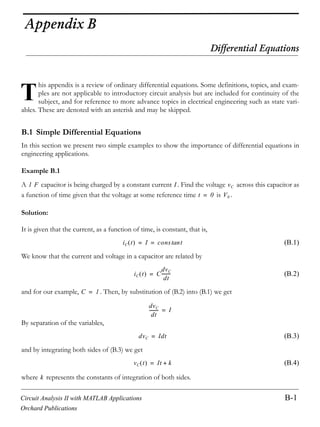
442. Differential Equations
B-12 Circuit Analysis II with MATLAB Applications
Orchard Publications
The function is shown in Figure B.1 plotted with the MATLAB command ezplot(y,[0 10]).
Figure B.1. Plot for the function of Example B.6.
Example B.7
Find the total solution of the ODE
(B.36)
subject to the initial conditions and
Solution:
The left side of (B.36) is the same as that of Example B.6.Therefore,
(B.37)
(We must remember that the constants and must be evaluated from the total response).
To find the forced response, we assume a solution of the form
(B.38)
We can find out whether our assumption is correct by substituting (B.38) into the given ODE of
(B.36). Then,
(B.39)
y f t=
y f t=
t
2
2
d
d y
4
dy
dt
------ 3y+ + 3e
2t–
=
y 0 1= y' 0 1–=
yN t k1e
t–
k2e
3t–
+=
k1 k2
yF Ae
2t–
=
4Ae
2t–
8Ae
2t–
– 3Ae
2t–
+ 3e
2t–
=

443. Circuit Analysis II with MATLAB Applications B-13
Orchard Publications
Using the Method of Undetermined Coefficients for the Forced Response
from which and the total solution is
(B.40)
The constants and are evaluated from the given initial conditions. For this example,
or
(B.41)
Also,
or
Simultaneous solution of (B.41) and (B.42) yields and . By substitution into (B.40),
we get
(B.42)
Check with MATLAB:
y=dsolve('D2y+4*Dy+3*y=3*exp( 2*t)', 'y(0)=1', 'Dy(0)= 1')
y =
(-3*exp(-2*t)*exp(t)+3/2*exp(-3*t)*exp(t)+5/2)/exp(t)
pretty(y)
-3 exp(-2 t) exp(t) + 3/2 exp(-3 t) exp(t) + 5/2
------------------------------------------------
exp(t)
ezplot(y,[0 8])
The plot is shown in Figure B.2
Example B.8
Find the total solution of the ODE
(B.43)
subject to the initial conditions and
A 3–=
y t yN yF+ k1e
t–
k2e
3t–
3– e
2t–
+= =
k1 k2
y 0 1 k1e
0
k2e
0
3e
0
–+= =
k1 k2+ 4=
y' 0 1– dy
dt
------
t 0=
k1e
t–
– 3k2e
3t–
– 6e
2t–
+ t 0=
= = =
k1– 3k2– 7–=
k1 2.5= k2 1.5=
y t yN yF+ 2.5e
t–
1.5e
3t–
3– e
2t–
+= =
t
2
2
d
d y 6
dy
dt
------ 9y+ + 0=
y 0 1–= y' 0 1=

444. Differential Equations
B-14 Circuit Analysis II with MATLAB Applications
Orchard Publications
Figure B.2. Plot for the function of Example B.7.
Solution:
This is a homogeneous ODE and therefore its total solution is just the natural response found from
the characteristic equation whose roots are (repeated roots). Thus, the
total response is
(B.44)
Next, we evaluate the constants and from the given initial conditions. For this example,
or
(B.45)
Also,
or
(B.46)
From (B.45) and (B.46) we get yields and . By substitution into (B.44),
(B.47)
y f t=
s
2
6s 9+ + 0= s1 s2 3–= =
y t yN k1e
3t–
k2 te
3t–
+= =
k1 k2
y 0 1– k1e
0
k2 0 e
0
+= =
k1 1–=
y' 0 1 dy
dt
------
t 0=
3k1e
3t–
– k2e
3t–
3k2te
3t–
–+ t 0=
= = =
3k1– k2+ 1=
k1 1–= k2 2–=
y t e–
3t–
2te
3t–
–=

445. Circuit Analysis II with MATLAB Applications B-15
Orchard Publications
Using the Method of Undetermined Coefficients for the Forced Response
Check with MATLAB:
y=dsolve('D2y+6*Dy+9*y=0', 'y(0)= 1', 'Dy(0)=1')
y =
-exp(-3*t)-2*exp(-3*t)*t
ezplot(y,[0 4])
The plot is shown in Figure B.3.
Figure B.3. Plot for the function of Example B.8.
Example B.9
Find the total solution of the ODE
(B.48)
Solution:
No initial conditions are given; therefore, we will express the solution in terms of the constants
and . By inspection, the roots of the characteristic equation of (B.48) are and
and thus the natural response has the form
(B.49)
Next, we find the forced response by assuming a solution of the form
(B.50)
y f t=
t
2
2
d
d y
5
dy
dt
------ 6y+ + 3e
2t–
=
k1
k2 s1 2–= s2 3–=
yN k1e
2t–
k2 e
3t–
+=
yF Ae
2t–
=

446. Differential Equations
B-16 Circuit Analysis II with MATLAB Applications
Orchard Publications
We can find out whether our assumption is correct by substitution of (B.50) into the given ODE of
(B.48). Then,
(B.51)
but the sum of the three terms on the left side of (B.52) is zero whereas the right side can never be
zero unless we let t and this produces a meaningless result.
The problem here is that the right side of the given ODE of (B.48) has the same form as one of the
terms of the natural response of (B.49), namely the term .
To work around this problem, we assume that the forced response has the form
(B.52)
that is, we multiply (B.50) by in order to eliminate the duplication of terms in the total response.
Then, by substitution of (B.52) into (B.48) and equating like terms, we find that . Therefore,
the total response is
(B.53)
Check with MATLAB:
y=dsolve('D2y+5*Dy+6*y=3*exp(-2*t)')
y =
-3*exp(-2*t)+3*t*exp(-2*t)+C1*exp(-3*t)+C2*exp(-2*t)
Example B.10
Find the total solution of the ODE
(B.54)
Solution:
No initial conditions are given; therefore, we will express solution in terms of the constants and
. We observe that the left side of (B.54) is the same of that of Example B.9. Therefore, the natural
response is the same, that is, it has the form
(B.55)
Next, to find the forced response and we assume a solution of the form
(B.56)
4Ae
2t–
10Ae
2t–
– 6Ae
2t–
+ 3e
2t–
=
k1 e
2t–
yF Ate
2t–
=
t
A 3=
y t yN yF+ k1e
2t–
k2e
3t–
3te
2t–
+ += =
t
2
2
d
d y 5
dy
dt
------ 6y+ + 4 5tcos=
k1
k2
yN k1e
2t–
k2e
3t–
+=
yF A 5tcos=

447. Circuit Analysis II with MATLAB Applications B-17
Orchard Publications
Using the Method of Undetermined Coefficients for the Forced Response
We can find out whether our assumption is correct by substitution of the assumed solution of (B.56)
into the given ODE of (B.55). Then,
but this relation is invalid since by equating cosine and sine terms, we find that and also
. This inconsistency is a result of our failure to recognize that the derivatives of pro-
duce new terms of the form and these terms must be included in the forced response.
Accordingly, we let
(B.57)
and by substitution into (B.54) we get
Collecting like terms and equating sine and cosine terms, we obtain the following set of equations
(B.58)
We use MATLAB to solve (B.58)
format rat; [k3 k4]=solve(19*x+25*y, 25*x-19*y-4)
k3 =
50/493
k4 =
-38/493
Therefore, the total solution is
(B.59)
Check with MATLAB.
y=dsolve('D2y+5*Dy+6*y=4*cos(5*t)'); y=simple(y)
y =
-38/493*cos(5*t)+50/493*sin(5*t)+C1*exp(-3*t)+C2*exp(-2*t)
In most engineering problems the right side of the non-homogeneous ODE consists of elementary
functions such as (constant), where is a positive integer, , , , and linear combi-
nations of these. Table B.1 summarizes the forms of the forced response for a second order ODE
with constant coefficients.
25A 5tcos– 25A 5sin t– 6A 5tcos+ 19A 5tcos– 25A 5sin t– 4 5tcos= =
A 4– 19=
A 0= A 5tcos
B 5tsin
yF k3 5sin t k4 5tcos+=
25– k3 5tsin 25k4 5cos t 25k3 5cos t+– 25k4 5sin t–
6k3 5tsin 6k4 5cos t+ + 4 5cos t=
19k3 25k4+ 0=
25k3 19– k4 4=
y t yN yF t+ k1e
2t–
k2e
3t– 50
493
--------- 5tsin
38–
493
--------- 5tcos+ + += =
k x
n
n e
kx
kxcos kxsin

448. Differential Equations
B-18 Circuit Analysis II with MATLAB Applications
Orchard Publications
We must remember that if is the sum of several terms, the most general form of the forced
response is the linear combination of these terms. Also, if a term in is a duplicate of a
term in the natural response , we must multiply by the lowest power of that will elimi-
nate the duplication.
Example B.11
Find the total solution of the ODE
(B.60)
Solution:
No initial conditions are given; therefore we will express solution in terms of the constants and
. The roots of the characteristic equation are equal, that is, , and thus the natural
response has the form
(B.61)
To find the forced response (particular solution), we refer to the table of the previous page and from
the last row we choose the term . This term with , , and , reduces to
. Therefore the forced response will have the form
TABLE B.1 Form of the forced response for 2nd order differential equations
Forced Response of the ODE
Form of Forced Response
(constant) (constant)
( = positive integer)
( =real or complex)
or ( =constant)
or
+
a
d
2
y
dt
2
-------- b
dy
dt
------ cy+ + f t=
f t yF t
k K
k t
n
n K0 t
n
K1 t
n 1–
Kn 1– t Kn+ + + +
ke
rt
r Ke
rt
k tcos k tsin K1coa t K2 tsin+
k t
n
e
r t
tcos k t
n
e
r t
sin t K0 t
n
K1 t
n 1–
Kn 1– t Kn+ + + + e
rt
tcos
K0 t
n
K1 t
n 1–
Kn 1– t Kn+ + + + e
rt
tsin
f t
yF t yF t
yN t yF t t
t
2
2
d
d y 4
dy
dt
------ 4y+ + te
2t–
e
2t–
–=
k1
k2 s1 s2 2–= =
yN k1e
2– t
k2 te
2– t
+=
k t
n
e
r t
tcos n 1= r 2–= 0=
kte
2– t

449. Circuit Analysis II with MATLAB Applications B-19
Orchard Publications
Using the Method of Undetermined Coefficients for the Forced Response
(B.62)
But the terms and are also present in (B.61); therefore, we multiply (B.62) by to obtain a
suitable form for the forced response which now is
(B.63)
Now, we need to evaluate the constants and . This is done by substituting (B.63) into the given
ODE of (B.60) and equating with the right side. We use MATLAB do the computations as shown
below.
syms t k3 k4 % Define symbolic variables
f0=(k3*t^3+k4*t^2)*exp( 2*t); % Forced response (B.64)
f1=diff(f0); f1=simple(f1) % Compute and simplify first derivative
f1 =
-t*exp(-2*t)*(-3*k3*t-2*k4+2*k3*t^2+2*k4*t)
f2=diff(f0,2); f2=simple(f2) % Compute and simplify second derivative
f2 =
2*exp(-2*t)*(3*k3*t+k4-6*k3*t^2-4*k4*t+2*k3*t^3+2*k4*t^2)
f=f2+4*f1+4*f0; f=simple(f) % Form and simplify the left side of the given ODE
f = 2*(3*k3*t+k4)*exp(-2*t)
Finally, we equate f above with the right side of the given ODE, that is
(B.64)
and we find and . By substitution of these values into (B.64) and combining
the forced response with the natural response, we get the total solution
(B.65)
We verify this solution with MATLAB
z=dsolve('D2y+4*Dy+4*y=t*exp( 2*t) exp( 2*t)')
z =
1/6*exp(-2*t)*t^3-1/2*exp(-2*t)*t^2
+C1*exp(-2*t)+C2*t*exp(-2*t)
yF k3 t k4+ e
2– t
=
e
2t–
te
2t–
t
2
yF k3 t
3
k4 t
2
+ e
2– t
=
k3 k4
2 3k3 t k4+ e
2t–
te
2t–
e
2t–
–=
k3 1 6= k4 1 2–=
y t k1e
2– t
k2te
2– t 1
6
---t
3
e
2– t 1
2
---t
2
e
2– t
–+ +=

450. Differential Equations
B-20 Circuit Analysis II with MATLAB Applications
Orchard Publications
B.6 Using the Method of Variation of Parameters for the Forced Response
In certain non-homogeneous ODEs, the right side cannot be determined by the method of
undetermined coefficients. For these ODEs we must use the method of variation of parameters. This
method will work with all linear equations including those with variable coefficients such as
(B.66)
provided that the general form of the natural response is known.
Our discussion will be restricted to second order ODEs with constant coefficients.
The method of variation of parameters replaces the constants and by two variables and
that satisfy the following three relations:
(B.67)
(B.68)
(B.69)
Simultaneous solution of (B.68) and (B.69) will yield the values of and ; then, integra-
tion of these will produce and , which when substituted into (B.67) will yield the total solution.
Example B.12
Find the total solution of
(B.70)
in terms of the constants and by the
a. method of undetermined coefficients
b. method of variation of parameters
Solution:
With either method, we must first find the natural response. The characteristic equation yields the
roots and . Therefore, the natural response is
f t
d2y
dt
2
-------- t
dy
dt
------ t y+ + f t=
k1 k2 u1 u2
y u1 y1 u2 y2+=
du1
dt
------- y1
du2
dt
------- y2+ 0=
du1
dt
-------
dy1
dt
-------
du2
dt
--------
dy2
dt
--------+ f t=
du1 dt du2 dt
u1 u2
d2y
dt
2
-------- 4
dy
dt
------ 3y+ + 12=
k1 k2
s1 1–= s2 3–=

451. Circuit Analysis II with MATLAB Applications B-21
Orchard Publications
Using the Method of Variation of Parameters for the Forced Response
(B.71)
a. Using the method of undetermined coefficients we let (a constant). Then, by substitution
into (B.70) we get and thus the total solution is
(B.72)
b. With the method of variation of parameters we start with the natural response found above as
(B.71) and we let the solutions and be represented as
(B.73)
Then by (B.67), the total solution is
or
(B.74)
Also, from (B.68),
or
(B.75)
and from (B.69),
or
(B.76)
Next, we find and by Cramer’s rule as follows:
(B.77)
and
yN k1e
t–
k2 e
3– t
+=
yF k3=
k3 4=
y t yN yF+ k1e
t–
k2e
3– t
4+ += =
y1 y2
y1 e
t–
= and y2 e
3t–
=
y u1y1 u2y2+=
y u1e
t–
u2e
3t–
+=
du1
dt
--------y1
du2
dt
--------y2+ 0=
du1
dt
--------e
t– du2
dt
--------e
3t–
+ 0=
du1
dt
-------
dy1
dt
-------
du2
dt
--------
dy2
dt
--------+ f t=
du1
dt
-------- e
t–
–
du2
dt
-------- 3e
3t–
–+ 12=
du1 dt du2 dt
du1
dt
--------
0 e
3t–
12 3e
3t–
–
e
t–
e
3t–
e
t–
– 3e
3t–
–
------------------------------------------ 12e
3t–
–
3e
4t–
– e
4t–
+
------------------------------ 12e
3t–
–
2e
4t–
–
----------------- 6e
t
= = = =

452. Differential Equations
B-22 Circuit Analysis II with MATLAB Applications
Orchard Publications
(B.78)
Now, integration of (B.77) and (B.78) and substitution into (B.75) yields
(B.79)
(B.80)
We observe that the last expression in (B.80) is the same as (B.72) of part (a).
Check with MATLAB:
y=dsolve('D2y+4*Dy+3*y=12')
y =
(4*exp(t)+C1*exp(-3*t)*exp(t)+C2)/exp(t)
Example B.13
Find the total solution of
(B.81)
in terms of the constants and by any method.
Solution:
This ODE cannot be solved by the method of undetermined coefficients; therefore, we will use the
method of variation of parameters.
The characteristic equation is from which and thus the natural response is
(B.82)
We let
(B.83)
du2
dt
--------
e
t–
0
e
t–
– 12
2e
4t–
–
--------------------------------- 12e
t–
2e
4t–
–
-------------- 6– e
3t
= = =
u1 6 e
t
td 6e
t
k1+= = u2 6– e
3t
td 2– e
3t
k2+= =
y u1e
t–
u2e
3t–
+=
6e
t
k1+ e
t–
2– e
3t
k2+ e
3t–
+=
6 k1e
t–
2 k2e
3t–
+–+=
k1e
t–
k2e
3t–
4+ +=
d
2
y
dt
2
-------- 4y+ 2ttan=
k1 k2
s
2
4+ 0= s j2=
yN k1e
j2t
k2e
j– 2t
+=
y1 2tcos= and y2 2tsin=

453. Circuit Analysis II with MATLAB Applications B-23
Orchard Publications
Using the Method of Variation of Parameters for the Forced Response
Then, by (B.67) the solution is
(B.84)
Also, from (B.68),
or
(B.85)
and from (B.69),
(B.86)
Next, we find and by Cramer’s rule as follows:
(B.87)
and
(B.88)
Now, integration of (B.87) and (B.88) and substitution into (B.84) yields
(B.89)
(B.90)
(B.91)
Check with MATLAB:
y=dsolve('D2y+4*y=tan(2*t)')
y =
-1/4*cos(2*t)*log((1+sin(2*t))/cos(2*t))+C1*cos(2*t)+C2*sin(2*t)
y u1y1 u2y2+ u1 2tcos u2 2tsin+= =
du1
dt
-------y1
du2
dt
--------y2+ 0=
du1
dt
------- 2tcos
du2
dt
-------- 2tsin+ 0=
du1
dt
-------
dy1
dt
-------
du2
dt
--------
dy2
dt
--------+ f t
du1
dt
-------= = 2 2tsin–
du2
dt
-------- 2 2tcos+ 2ttan=
du1 dt du2 dt
du1
dt
-------
0 2tsin
2ttan 2 2tcos
2tcos 2tsin
2 2tsin– 2 2tcos
------------------------------------------------------
2t
2
sin
2tcos
--------------–
2 2t
2
cos 2 2t
2
sin+
------------------------------------------- 2t
2
sin–
2 2tcos
------------------= = =
du2
dt
--------
2tcos 0
2 2tsin– 2ttan
2
--------------------------------------------------- 2tsin
2
------------= =
u1
1
2
---–
2t
2
sin
2tcos
-------------- td
2tsin
4
------------
1
4
--- 2tsec 2ttan+ln– k1+= =
u2
1
2
--- 2tsin td 2tcos
4
-------------– k2+= =
y u1y1 u2y2+
2t 2tcossin
4
---------------------------
1
4
--- 2t 2tsec 2ttan+lncos– k1 2tcos+
2t 2tcossin
4
---------------------------– k2 2tsin+= =
1
4
--- 2t 2tsec 2ttan+lncos– k1 2tcos k2 2tsin+ +=

454. Differential Equations
B-24 Circuit Analysis II with MATLAB Applications
Orchard Publications
B.7 Exercises
Solve the following ODEs by any method.
1.
Answer:
2.
Answer:
3. Hint: Use
Answer:
4.
Answer:
d
2
y
dt
2
-------- 4
dy
dt
------ 3y+ + t 1–=
y k1e
t–
k2e
3t– 1
3
---t
7
9
---–+ +=
d
2
y
dt
2
-------- 4
dy
dt
------ 3y+ + 4e
t–
=
y k1e
t–
k2e
3t–
2te
t–
+ +=
d
2
y
dt
2
-------- 2
dy
dt
------ y+ + t
2
cos= t
2
cos
1
2
--- 2t 1+cos=
y k1e
t–
k2te
t– 1
2
---
3 2tcos 4 2tsin–
50
---------------------------------------–+ +=
d
2
y
dt
2
-------- y+ tsec=
y k1 tcos k2 tsin t tsin t tcoslncos+ + +=

455. Circuit Analysis II with MATLAB Applications C-1
Orchard Publications
Appendix C
Matrices and Determinants
his appendix is an introduction to matrices and matrix operations. Determinants, Cramer’s
rule, and Gauss’s elimination method are reviewed. Some definitions and examples are not
applicable to subsequent material presented in this text, but are included for subject continuity,
and reference to more advance topics in matrix theory. These are denoted with a dagger (†) and may
be skipped.
C.1 Matrix Definition
A matrix is a rectangular array of numbers such as those shown below.
In general form, a matrix A is denoted as
(C.1)
The numbers are the elements of the matrix where the index i indicates the row, and j indicates
the column in which each element is positioned. Thus, indicates the element positioned in the
fourth row and third column.
A matrix of m rows and n columns is said to be of order matrix.
If , the matrix is said to be a square matrix of order m (or n). Thus, if a matrix has five rows
and five columns, it is said to be a square matrix of order 5.
In a square matrix, the elements are called the main diagonal elements. Alter-
nately, we say that the matrix elements , are located on the main diagonal.
T
2 3 7
1 1– 5
or
1 3 1
2– 1 5–
4 7– 6
A
a11 a12 a13 a1n
a21 a22 a23 a2n
a31 a32 a33 a3n
am1 am2 am3 amn
=
aij
a43
m n
m n=
a11 a22 a33 ann
a11 a22 a33 ann

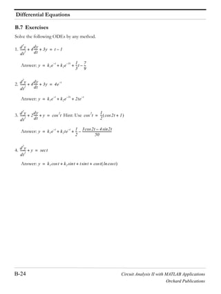
456. Appendix C Matrices and Determinants
C-2 Circuit Analysis II with MATLAB Applications
Orchard Publications
† The sum of the diagonal elements of a square matrix is called the trace*
of .
† A matrix in which every element is zero, is called a zero matrix.
C.2 Matrix Operations
Two matrices and are equal, that is, , if and only if
(C.2)
Two matrices are said to be conformable for addition (subtraction), if they are of the same order m n.
If and are conformable for addition (subtraction), their sum (difference) will be
another matrix with the same order as and , where each element of is the sum (difference)
of the corresponding elements of and , that is,
(C.3)
Example C.1
Compute and given that
and
Solution:
and
Check with MATLAB:
A=[1 2 3; 0 1 4]; B=[2 3 0; 1 2 5]; % Define matrices A and B
A+B % Add A and B
* Henceforth, all paragraphs and topics preceded by a dagger ( † ) may be skipped. These are discussed in matrix
theory textbooks.
A A
A aij
= B bij
= A B=
aij bij= i 1 2 3 m= j 1 2 3 n=
A aij
= B bij
=
C A B C
A B
C A B aij bij= =
A B+ A B–
A 1 2 3
0 1 4
= B 2 3 0
1– 2 5
=
A B+ 1 2+ 2 3+ 3 0+
0 1– 1 2+ 4 5+
3 5 3
1– 3 9
= =
A B– 1 2– 2 3– 3 0–
0 1+ 1 2– 4 5–
1– 1– 3
1 1– 1–
= =

457. Circuit Analysis II with MATLAB Applications C-3
Orchard Publications
Matrix Operations
ans =
3 5 3
-1 3 9
A B % Subtract B from A
ans =
-1 -1 3
1 -1 -1
If is any scalar (a positive or negative number), and not [k] which is a matrix, then multipli-
cation of a matrix by the scalar is the multiplication of every element of by .
Example C.2
Multiply the matrix
by
a.
b.
Solution:
a.
b.
Check with MATLAB:
k1=5; k2=( 3 + 2*j); % Define scalars k1 and k2
A=[1 2; 2 3]; % Define matrix A
k1*A % Multiply matrix A by constant k1
ans =
5 -10
10 15
k 1 1
A k A k
A 1 2–
2 3
=
k1 5=
k2 3– j2+=
k1 A 5 1 2–
2 3
5 1 5 2–
5 2 5 3
5 10–
10 15
= = =
k2 A 3– j2+ 1 2–
2 3
3– j2+ 1 3– j2+ 2–
3– j2+ 2 3– j2+ 3
3– j2+ 6 j4–
6– j4+ 9– j6+
= = =

458. Appendix C Matrices and Determinants
C-4 Circuit Analysis II with MATLAB Applications
Orchard Publications
k2*A %Multiply matrix A by constant k2
ans =
-3.0000+ 2.0000i 6.0000- 4.0000i
-6.0000+ 4.0000i -9.0000+ 6.0000i
Two matrices and are said to be conformable for multiplication in that order, only when the
number of columns of matrix is equal to the number of rows of matrix . That is, the product
(but not ) is conformable for multiplication only if is an matrix and matrix is
an matrix. The product will then be an matrix. A convenient way to determine if
two matrices are conformable for multiplication is to write the dimensions of the two matrices side-
by-side as shown below.
For the product we have:
For matrix multiplication, the operation is row by column. Thus, to obtain the product , we
multiply each element of a row of by the corresponding element of a column of ; then, we add
these products.
Example C.3
Matrices and are defined as
and
Compute the products and
A B A B
A B
A B B A A m p B
p n A B m n
m p p n
A B
Shows that A and B are conformable for multiplication
Indicates the dimension of the product A B
B A
Here, B and A are not conformable for multiplication
B A
p n m p
A B
A B
C D
C 2 3 4= D
1
1–
2
=
C D D C

459. Circuit Analysis II with MATLAB Applications C-5
Orchard Publications
Special Forms of Matrices
Solution:
The dimensions of matrices and are respectively ; therefore the product is
feasible, and will result in a , that is,
The dimensions for and are respectively and therefore, the product is also
feasible. Multiplication of these will produce a matrix as follows:
Check with MATLAB:
C=[2 3 4]; D=[1; 1; 2]; % Define matrices C and D
C*D % Multiply C by D
ans =
7
D*C % Multiply D by C
ans =
2 3 4
-2 -3 -4
4 6 8
Division of one matrix by another, is not defined. However, an equivalent operation exists, and it
will become apparent later in this chapter, when we discuss the inverse of a matrix.
C.3 Special Forms of Matrices
† A square matrix is said to be upper triangular when all the elements below the diagonal are zero.
The matrix of (C.4) is an upper triangular matrix.
In an upper triangular matrix, not all elements above the diagonal need to be non-zero.
C D 1 3 3 1 C D
1 1
C D 2 3 4
1
1–
2
2 1 3 1– 4 2+ + 7= = =
D C 3 1 1 3 D C
3 3
D C
1
1–
2
2 3 4
1 2 1 3 1 4
1– 2 1– 3 1– 4
2 2 2 3 2 4
2 3 4
2– 3– 4–
4 6 8
= = =
A

460. Appendix C Matrices and Determinants
C-6 Circuit Analysis II with MATLAB Applications
Orchard Publications
(C.4)
† A square matrix is said to be lower triangular, when all the elements above the diagonal are zero.
The matrix of (C.5) is a lower triangular matrix.
(C.5)
In a lower triangular matrix, not all elements below the diagonal need to be non-zero.
† A square matrix is said to be diagonal, if all elements are zero, except those in the diagonal. The
matrix of (C.6) is a diagonal matrix.
(C.6)
† A diagonal matrix is called a scalar matrix, if where k is a sca-
lar. The matrix of (C.7) is a scalar matrix with k = 4.
(C.7)
A scalar matrix with , is called an identity matrix . Shown below are , , and
identity matrices.
A
a11 a12 a13 a1n
0 a22 a23 a2n
0 0
0
0 0 0 amn
=
B
B
a11 0 0 0
a21 a22 0 0
0 0
0
am1 am2 am3 amn
=
C
C
a11 0 0 0
0 a22 0 0
0 0 0 0
0 0 0 0
0 0 0 amn
=
a11 a22 a33 ann k= = = = =
D
D
4 0 0 0
0 4 0 0
0 0 4 0
0 0 0 4
=
k 1= I 2 2 3 3 4 4

461. Circuit Analysis II with MATLAB Applications C-7
Orchard Publications
Special Forms of Matrices
(C.8)
The MATLAB eye(n) function displays an identity matrix. For example,
eye(4) % Display a 4 by 4 identity matrix
ans =
1 0 0 0
0 1 0 0
0 0 1 0
0 0 0 1
Likewise, the eye(size(A)) function, produces an identity matrix whose size is the same as matrix
. For example, let matrix be defined as
A=[1 3 1; 2 1 5; 4 7 6] % Define matrix A
A =
1 3 1
-2 1 -5
4 -7 6
then,
eye(size(A))
displays
ans =
1 0 0
0 1 0
0 0 1
† The transpose of a matrix , denoted as , is the matrix that is obtained when the rows and col-
umns of matrix are interchanged. For example, if
(C.9)
1 0
0 1
1 0 0
0 1 0
0 0 1
1 0 0 0
0 1 0 0
0 0 1 0
0 0 0 1
n n
A A
A A
T
A
A
1 2 3
4 5 6
= then A
T
1 4
2 5
3 6
=

462. Appendix C Matrices and Determinants
C-8 Circuit Analysis II with MATLAB Applications
Orchard Publications
In MATLAB we use the apostrophe ( ) symbol to denote and obtain the transpose of a matrix. Thus,
for the above example,
A=[1 2 3; 4 5 6] % Define matrix A
A =
1 2 3
4 5 6
A' % Display the transpose of A
ans =
1 4
2 5
3 6
† A symmetric matrix is a matrix such that , that is, the transpose of a matrix is the same
as . An example of a symmetric matrix is shown below.
(C.10)
† If a matrix has complex numbers as elements, the matrix obtained from by replacing each
element by its conjugate, is called the conjugate of , and it is denoted as
An example is shown below.
MATLAB has two built-in functions which compute the complex conjugate of a number. The
first, conj(x), computes the complex conjugate of any complex number, and the second, conj(A),
computes the conjugate of a matrix . Using MATLAB with the matrix defined as above, we
get
A = [1+2j j; 3 2 3j] % Define and display matrix A
A =
1.0000+ 2.0000i 0+ 1.0000i
3.0000 2.0000- 3.0000i
conj_A=conj(A) % Compute and display the conjugate of A
conj_A =
1.0000- 2.0000i 0- 1.0000i
A A
T
A= A
A
A
1 2 3
2 4 5–
3 5– 6
= A
T
1 2 3
2 4 5–
3 5– 6
A= =
A A
A A
A 1 j2+ j
3 2 j3–
= A 1 j2– j–
3 2 j3+
=
A A

463. Circuit Analysis II with MATLAB Applications C-9
Orchard Publications
Determinants
3.0000 2.0000+ 3.0000i
† A square matrix such that is called skew-symmetric. For example,
Therefore, matrix above is skew symmetric.
† A square matrix such that is called Hermitian. For example,
Therefore, matrix above is Hermitian.
† A square matrix such that is called skew Hermitian. For example,
Therefore, matrix above is skew-Hermitian.
C.4 Determinants
Let matrix be defined as the square matrix
(C.11)
then, the determinant of , denoted as , is defined as
(C.12)
A A
T
A–=
A
0 2 3–
2– 0 4–
3 4 0
= A
T
0 2– 3
2 0 4
3– 4– 0
A–= =
A
A A
T
A=
A
1 1 j– 2
1 j+ 3 j
2 j– 0
A
T
1 1 j+ 2
1 j– 3 j–
2 j 0
A
T*
1 1 j+ 2
1 j– 3 j–
2 j 0
A====
A
A A
T
A–=
A
j 1 j– 2
1– j– 3j j
2– j 0
A
T
j 1– j– 2–
1 j– 3j j
2 j 0
A
T*
j– 1– j+ 2–
1 j+ 3j– j–
2 j– 0
A–====
A
A
A
a11 a12 a13 a1n
a21 a22 a23 a2n
a31 a32 a33 a3n
an1 an2 an3 ann
=
A detA
detA a11a22a33 ann a12a23a34 an1
a13a24a35 an2
an1
a22a13 an2
– a23a14 an3
a24a15 –––
+ + +=

464. Appendix C Matrices and Determinants
C-10 Circuit Analysis II with MATLAB Applications
Orchard Publications
The determinant of a square matrix of order n is referred to as determinant of order n.
Let be a determinant of order 2, that is,
(C.13)
Then,
(C.14)
Example C.4
Matrices and are defined as
and
Compute and .
Solution:
Check with MATLAB:
A=[1 2; 3 4]; B=[2 1; 2 0]; % Define matrices A and B
det(A) % Compute the determinant of A
ans =
-2
det(B) % Compute the determinant of B
ans =
2
Let be a matrix of order 3, that is,
(C.15)
then, is found from
A
A
a11 a12
a21 a22
=
detA a11a22 a21a12–=
A B
A 1 2
3 4
= B 2 1–
2 0
=
detA detB
detA 1 4 3 2– 4 6– 2–= = =
detB 2 0 2 1–– 0 2–– 2= = =
A
A
a11 a12 a13
a21 a22 a23
a31 a32 a33
=
detA

465. Circuit Analysis II with MATLAB Applications C-11
Orchard Publications
Determinants
(C.16)
A convenient method to evaluate the determinant of order 3, is to write the first two columns to the
right of the 3 3 matrix, and add the products formed by the diagonals from upper left to lower
right; then subtract the products formed by the diagonals from lower left to upper right as shown
on the diagram of the next page. When this is done properly, we obtain (C.16) above.
This method works only with second and third order determinants. To evaluate higher order deter-
minants, we must first compute the cofactors; these will be defined shortly.
Example C.5
Compute and if matrices and are defined as
and
Solution:
or
Likewise,
or
Check with MATLAB:
detA a11a22a33 a12a23a31 a11a22a33+ +=
a11a22a33 a11a22a33 a11a22a33–––
a11 a12 a13
a21 a22 a23
a31 a32 a33
a11 a12
a21 a22
a31 a32 +
detA detB A B
A
2 3 5
1 0 1
2 1 0
= B
2 3– 4–
1 0 2–
0 5– 6–
=
detA
2 3 5 2 3
1 0 1 1 0
2 1 0 2 1
=
detA 2 0 0 3 1 1 5 1 1
2 0 5– 1 1 2 0 1 3––
+ +
11 2– 9= =
=
detB
2 3– 4– 2 3–
1 0 2– 1 2–
0 5– 6– 2 6–
=
detB 2 0 6– 3– 2– 0 4– 1 5–
0 0 4–– 5– 2– 2 6– 1 3–––
+ +
20 38– 18–= =
=

466. Appendix C Matrices and Determinants
C-12 Circuit Analysis II with MATLAB Applications
Orchard Publications
A=[2 3 5; 1 0 1; 2 1 0]; det(A) % Define matrix A and compute detA
ans =
9
B=[2 3 4; 1 0 2; 0 5 6];det(B) % Define matrix B and compute detB
ans =
-18
C.5 Minors and Cofactors
Let matrix be defined as the square matrix of order n as shown below.
(C.17)
If we remove the elements of its ith row, and jth column, the remaining square matrix is called
the minor of , and it is denoted as .
The signed minor is called the cofactor of and it is denoted as .
Example C.6
Matrix is defined as
(C.18)
Compute the minors , , and the cofactors , and .
Solution:
A
A
a11 a12 a13 a1n
a21 a22 a23 a2n
a31 a32 a33 a3n
an1 an2 an3 ann
=
n 1–
A Mij
1–
i j+
Mij
aij ij
A
A
a11 a12 a13
a21 a22 a23
a31 a32 a33
=
M11 M12 M13 11 12 13

467. Circuit Analysis II with MATLAB Applications C-13
Orchard Publications
Minors and Cofactors
and
The remaining minors
and cofactors
are defined similarly.
Example C.7
Compute the cofactors of matrix defined as
(C.19)
Solution:
(C.20)
(C.21)
(C.22)
(C.23)
(C.24)
It is useful to remember that the signs of the cofactors follow the pattern
M11
a22 a23
a32 a33
= M12
a21 a23
a31 a33
= M11
a21 a22
a31 a32
=
11 1–
1 1+
M11 M11 12 1–
1 2+
M12 M12 13 M13
1–
1 3+
M13
= =–= == =
M21 M22 M23 M31 M32 M33
21 22 23 31 32 and 33
A
A
1 2 3–
2 4– 2
1– 2 6–
=
11 1–
1 1+ 4– 2
2 6–
20= = 12 1–
1 2+ 2 2
1– 6–
10= =
13 1–
1 3+ 2 4–
1– 2
0 21 1–
2 1+ 2 3–
2 6–
6= == =
22 1–
2 2+ 1 3–
1– 6–
9–= = 23 1–
2 3+ 1 2
1– 2
4–= =
31 1–
3 1+ 2 3–
4– 2
8–= = 32 1–
3 2+ 1 3–
2 2
8–= =
33 1–
3 3+ 1 2
2 4–
8–= =

468. Appendix C Matrices and Determinants
C-14 Circuit Analysis II with MATLAB Applications
Orchard Publications
that is, the cofactors on the diagonals have the same sign as their minors.
Let be a square matrix of any size; the value of the determinant of is the sum of the products
obtained by multiplying each element of any row or any column by its cofactor.
Example C.8
Matrix is defined as
(C.25)
Compute the determinant of using the elements of the first row.
Solution:
Check with MATLAB:
A=[1 2 3; 2 4 2; 1 2 6];det(A) % Define matrix A and compute detA
ans =
40
We must use the above procedure to find the determinant of a matrix of order 4 or higher. Thus, a
fourth-order determinant can first be expressed as the sum of the products of the elements of its first
row by its cofactor as shown below.
+ + +
+ +
+ + +
+ +
+ + +
A A
A
A
1 2 3–
2 4– 2
1– 2 6–
=
A
detA 1 4– 2
2 6–
= 2 2 2
1– 6–
3 2 4–
1– 2
–– 1 20 2 10– 3 0–– 40= =
A

469. Circuit Analysis II with MATLAB Applications C-15
Orchard Publications
Minors and Cofactors
(C.26)
Determinants of order five or higher can be evaluated similarly.
Example C.9
Compute the value of the determinant of the matrix defined as
(C.27)
Solution:
Using the above procedure, we will multiply each element of the first column by its cofactor. Then,
Next, using the procedure of Example C.5 or Example C.8, we find
, , ,
and thus
We can verify our answer with MATLAB as follows:
A=[ 2 1 0 3; 1 1 0 1; 4 0 3 2; 3 0 0 1]; delta = det(A)
delta =
-33
A
a11 a12 a13 a14
a21 a22 a23 a24
a31 a32 a33 a34
a41 a42 a43 a44
a11
a22 a23 a24
a32 a33 a34
a42 a43 a44
a21
a12 a13 a14
a32 a33 a34
a42 a43 a44
–
+a31
a12 a13 a14
a22 a23 a24
a42 a43 a44
a41
a12 a13 a14
a22 a23 a24
a32 a33 a34
–
= =
A
A
2 1– 0 3–
1– 1 0 1–
4 0 3 2–
3– 0 0 1
=
A=2
1 0 1–
0 3 2–
0 0 1
a
1–
1– 0 3–
0 3 2–
0 0 1
–
b
+4
1– 0 3–
1 0 1–
0 0 1
c
3–
1– 0 3–
1 0 1–
0 3 2–
–
d
a 6= b 3–= c 0= d 36–=
detA a b c d+ + + 6 3– 0 36–+ 33–= = =

470. Appendix C Matrices and Determinants
C-16 Circuit Analysis II with MATLAB Applications
Orchard Publications
Some useful properties of determinants are given below.
Property 1: If all elements of one row or one column are zero, the determinant is zero. An example of
this is the determinant of the cofactor above.
Property 2: If all the elements of one row or column are m times the corresponding elements of another
row or column, the determinant is zero. For example, if
(C.28)
then,
(C.29)
Here, is zero because the second column in is 2 times the first column.
Check with MATLAB:
A=[2 4 1; 3 6 1; 1 2 1];det(A)
ans =
0
Property 3: If two rows or two columns of a matrix are identical, the determinant is zero. This follows
from Property 2 with .
C.6 Cramer’s Rule
Let us consider the systems of the three equations below
(C.30)
and let
c
A
2 4 1
3 6 1
1 2 1
=
detA
2 4 1
3 6 1
1 2 1
2 4
3 6
1 2
12 4 6 6 4–– 12–+ + 0= = =
detA A
m 1=
a11x a12y a13z+ + A=
a21x a22y a23z+ + B=
a31x a32y a33z+ + C=
a11 a12 a13
a21 a22 a23
a31 a32 a33
D1
A a11 a13
B a21 a23
C a31 a33
D2
a11 A a13
a21 B a23
a31 C a33
D3
a11 a12 A
a21 a22 B
a31 a32 C
====

471. Circuit Analysis II with MATLAB Applications C-17
Orchard Publications
Cramer’s Rule
Cramer’s rule states that the unknowns x, y, and z can be found from the relations
(C.31)
provided that the determinant (delta) is not zero.
We observe that the numerators of (C.31) are determinants that are formed from by the substitu-
tion of the known values , , and , for the coefficients of the desired unknown.
Cramer’s rule applies to systems of two or more equations.
If (C.30) is a homogeneous set of equations, that is, if , then, are
all zero as we found in Property 1 above. Then, also.
Example C.10
Use Cramer’s rule to find , , and if
(C.32)
and verify your answers with MATLAB.
Solution:
Rearranging the unknowns v, and transferring known values to the right side, we get
(C.33)
Now, by Cramer’s rule,
x
D1
------= y
D2
------= z
D3
------=
A B C
A B C 0= = = D1 D2 and D3
x y z 0= = =
v1 v2 v3
2v1 5– v2– 3v3+ 0=
2v3 3v2 4v1––– 8=
v2 3v1 4– v3–+ 0=
2v1 v2– 3v3+ 5=
4v1 3v2 2v3––– 8=
3v1 v2 v3–+ 4=
2 1– 3
4– 3– 2–
3 1 1–
2 1–
4– 3–
3 1
6 6 12– 27 4 4+ + + + 35= = =
D1
5 1– 3
8 3– 2–
4 1 1–
5 1–
8 3–
4 1
15 8 24 36 10 8–+ + + + 85= = =

472. Appendix C Matrices and Determinants
C-18 Circuit Analysis II with MATLAB Applications
Orchard Publications
Then, using (C.31) we get
(C.34)
We will verify with MATLAB as follows.
% The following code will compute and display the values of v1, v2 and v3.
format rat % Express answers in ratio form
B=[2 1 3; 4 3 2; 3 1 1]; % The elements of the determinant D of matrix B
delta=det(B); % Compute the determinant D of matrix B
d1=[5 -1 3; 8 -3 -2; 4 1 -1]; % The elements of D1
detd1=det(d1); % Compute the determinant of D1
d2=[2 5 3; -4 8 -2; 3 4 -1]; % The elements of D2
detd2=det(d2); % Compute the determinant of D2
d3=[2 -1 5; -4 -3 8; 3 1 4]; % The elements of D3
detd3=det(d3); % Compute he determinant of D3
v1=detd1/delta; % Compute the value of v1
v2=detd2/delta; % Compute the value of v2
v3=detd3/delta; % Compute the value of v3
%
disp('v1=');disp(v1); % Display the value of v1
disp('v2=');disp(v2); % Display the value of v2
disp('v3=');disp(v3); % Display the value of v3
v1=
17/7
v2=
-34/7
v3=
-11/7
These are the same values as in (C.34)
D2
2 5 3
4– 8 2–
3 4 1–
2 5
4– 8
3 4
16– 30– 48– 72– 16 20–+ 170–= = =
D3
2 1– 5
4– 3– 8
3 1 4
2 1–
4– 3–
3 1
24– 24– 20– 45 16– 16–+ 55–= = =
x1
D1
------ 85
35
------ 17
7
------= = = x2
D2
------ 170
35
---------– 34
7
------–= = = x3
D3
------ 55
35
------– 11
7
------–= = =

473. Circuit Analysis II with MATLAB Applications C-19
Orchard Publications
Gaussian Elimination Method
C.7 Gaussian Elimination Method
We can find the unknowns in a system of two or more equations also by the Gaussian elimination
method. With this method, the objective is to eliminate one unknown at a time. This can be done by
multiplying the terms of any of the equations of the system by a number such that we can add (or
subtract) this equation to another equation in the system so that one of the unknowns will be elimi-
nated. Then, by substitution to another equation with two unknowns, we can find the second
unknown. Subsequently, substitution of the two values found can be made into an equation with
three unknowns from which we can find the value of the third unknown. This procedure is repeated
until all unknowns are found. This method is best illustrated with the following example which con-
sists of the same equations as the previous example.
Example C.11
Use the Gaussian elimination method to find , , and of the system of equations
(C.35)
Solution:
As a first step, we add the first equation of (C.35) with the third to eliminate the unknown v2 and we
obtain the following equation.
(C.36)
Next, we multiply the third equation of (C.35) by 3, and we add it with the second to eliminate .
Then, we obtain the following equation.
(C.37)
Subtraction of (C.37) from (C.36) yields
(C.38)
Now, we can find the unknown from either (C.36) or (C.37). By substitution of (C.38) into (C.36)
we get
(C.39)
Finally, we can find the last unknown from any of the three equations of (C.35). By substitution
into the first equation we get
v1 v2 v3
2v1 v2– 3v3+ 5=
4v1 3v2 2v3––– 8=
3v1 v2 v3–+ 4=
5v1 2v3+ 9=
v2
5v1 5v3– 20=
7v3 11 or v3
11
7
------–=–=
v1
5v1 2
11
7
------–+ 9 or v1
17
7
------==
v2

474. Appendix C Matrices and Determinants
C-20 Circuit Analysis II with MATLAB Applications
Orchard Publications
(C.40)
These are the same values as those we found in Example C.10.
The Gaussian elimination method works well if the coefficients of the unknowns are small integers,
as in Example C.11. However, it becomes impractical if the coefficients are large or fractional num-
bers.
C.8 The Adjoint of a Matrix
Let us assume that is an n square matrix and is the cofactor of . Then the adjoint of ,
denoted as , is defined as the n square matrix below.
(C.41)
We observe that the cofactors of the elements of the ith row (column) of are the elements of the
ith column (row) of .
Example C.12
Compute if Matrix is defined as
(C.42)
Solution:
v2 2v1 3v3 5–+
34
7
------
33
7
------–
35
7
------–
34
7
------–= = =
A ij aij A
adjA
adjA
11 21 31 n1
12 22 32 n2
13 23 33 n3
1n 2n 3n nn
=
A
adjA
adjA A
A
1 2 3
1 3 4
1 4 3
=
adjA
3 4
4 3
2 3
4 3
– 2 3
3 4
1 4
1 3
– 1 3
1 3
2 3
3 4
–
1 3
1 4
1 2
1 4
– 1 2
1 3
7– 6 1–
1 0 1–
1 2– 1
= =

475. Circuit Analysis II with MATLAB Applications C-21
Orchard Publications
Singular and Non-Singular Matrices
C.9 Singular and Non-Singular Matrices
An n square matrix is called singular if ; if , is called non-singular.
Example C.13
Matrix is defined as
(C.43)
Determine whether this matrix is singular or non-singular.
Solution:
Therefore, matrix is singular.
C.10 The Inverse of a Matrix
If and are n square matrices such that , where is the identity matrix, is called
the inverse of , denoted as , and likewise, is called the inverse of , that is,
If a matrix is non-singular, we can compute its inverse from the relation
(C.44)
Example C.14
Matrix is defined as
(C.45)
Compute its inverse, that is, find
A detA 0= detA 0 A
A
A
1 2 3
2 3 4
3 5 7
=
detA
1 2 3
2 3 4
3 5 7
1 2
2 3
3 5
21 24 30 27– 20– 28–+ + 0= = =
A
A B AB BA I= = I B
A B A
1–
= A B A B
1–
=
A A
1–
A
1– 1
detA
------------adjA=
A
A
1 2 3
1 3 4
1 4 3
=
A
1–

476. Appendix C Matrices and Determinants
C-22 Circuit Analysis II with MATLAB Applications
Orchard Publications
Solution:
Here, , and since this is a non-zero value, it is possible to com-
pute the inverse of using (C.44).
From Example C.12,
Then,
(C.46)
Check with MATLAB:
A=[1 2 3; 1 3 4; 1 4 3], invA=inv(A) % Define matrix A and compute its inverse
A =
1 2 3
1 3 4
1 4 3
invA =
3.5000 -3.0000 0.5000
-0.5000 0 0.5000
-0.5000 1.0000 -0.5000
Multiplication of a matrix by its inverse produces the identity matrix , that is,
(C.47)
Example C.15
Prove the validity of (C.47) for the Matrix defined as
Proof:
detA 9 8 12 9– 16– 6–+ + 2–= =
A
adjA
7– 6 1–
1 0 1–
1 2– 1
=
A
1– 1
detA
------------adjA
1
2–
------
7– 6 1–
1 0 1–
1 2– 1
3.5 3– 0.5
0.5– 0 0.5
0.5– 1 0.5–
= = =
A A
1–
I
AA
1–
I or A
1–
A I==
A
A 4 3
2 2
=
detA 8 6– 2 and adjA 2 3–
2– 4
== =

477. Circuit Analysis II with MATLAB Applications C-23
Orchard Publications
Solution of Simultaneous Equations with Matrices
Then,
and
C.11 Solution of Simultaneous Equations with Matrices
Consider the relation
(C.48)
where and are matrices whose elements are known, and is a matrix (a column vector) whose
elements are the unknowns. We assume that and are conformable for multiplication. Multipli-
cation of both sides of (C.48) by yields:
(C.49)
or
(C.50)
Therefore, we can use (C.50) to solve any set of simultaneous equations that have solutions. We will
refer to this method as the inverse matrix method of solution of simultaneous equations.
Example C.16
For the system of the equations
(C.51)
compute the unknowns using the inverse matrix method.
Solution:
In matrix form, the given set of equations is where
A
1– 1
detA
------------adjA
1
2
--- 2 3–
2– 4
1 3– 2
1– 2
= = =
AA
1– 4 3
2 2
1 3– 2
1– 2
4 3– 6– 6+
2 2– 3– 4+
1 0
0 1
I= = = =
AX B=
A B X
A X
A
1–
A
1–
AX A
1–
B IX A
1–
B= = =
X=A
1–
B
2x1 3x2 x3+ + 9=
x1 2x2 3x3+ + 6=
3x1 x2 2x3+ + 8=
x1 x2 and x3
AX B=

478. Appendix C Matrices and Determinants
C-24 Circuit Analysis II with MATLAB Applications
Orchard Publications
(C.52)
Then,
(C.53)
or
(C.54)
Next, we find the determinant , and the adjoint
Therefore,
and by (C.53) we obtain the solution as follows.
(C.55)
To verify our results, we could use the MATLAB’s inv(A) function, and then multiply by B.
However, it is easier to use the matrix left division operation ; this is MATLAB’s solution
of for the matrix equation , where matrix X is the same size as matrix B. For this
example,
A=[2 3 1; 1 2 3; 3 1 2]; B=[9 6 8]';
X=A B
A
2 3 1
1 2 3
3 1 2
= X
x1
x2
x3
= B
9
6
8
=
X A
1–
B=
x1
x2
x3
2 3 1
1 2 3
3 1 2
1–
9
6
8
=
detA adjA
detA 18= and adjA
1 5– 7
7 1 5–
5– 7 1
=
A
1– 1
detA
------------ adjA
1
18
------
1 5– 7
7 1 5–
5– 7 1
= =
X
x1
x2
x3
1
18
------
1 5– 7
7 1 5–
5– 7 1
9
6
8
1
18
------
35
29
5
35 18
29 18
5 18
1.94
1.61
0.28
= = = = =
A
1–
X A B=
A
1–
B A X B=

479. Circuit Analysis II with MATLAB Applications C-25
Orchard Publications
Solution of Simultaneous Equations with Matrices
X =
1.9444
1.6111
0.2778
Example C.17
For the electric circuit of Figure C.1,
Figure C.1. Circuit for Example C.17
the loop equations are
(C.56)
Use the inverse matrix method to compute the values of the currents , , and
Solution:
For this example, the matrix equation is or , where
The next step is to find . This is found from the relation
(C.57)
Therefore, we find the determinant and the adjoint of . For this example, we find that
+
V = 100 v
9 9 4
221
I1 I3I2
10I1 9I2– 100=
9I1 20I2 9I3–+– 0=
9I2 15I3+– 0=
I1 I2 I3
RI V= I R
1–
V=
R
10 9– 0
9– 20 9–
0 9– 15
= V
100
0
0
and I
I1
I2
I3
==
R
1–
R
1– 1
detR
------------ adjR=
R

480. Appendix C Matrices and Determinants
C-26 Circuit Analysis II with MATLAB Applications
Orchard Publications
(C.58)
Then,
and
Check with MATLAB:
R=[10 9 0; 9 20 9; 0 9 15]; V=[100 0 0]'; I=RV
I =
22.4615
13.8462
8.3077
We can also use subscripts to address the individual elements of the matrix. Accordingly, the above
code could also have been written as:
R(1,1)=10; R(1,2)=-9; % No need to make entry for A(1,3) since it is zero.
R(2,1)=-9; R(2,2)=20; R(2,3)=-9; R(3,2)=-9; R(3,3)=15; V=[100 0 0]'; I=RV
I =
22.4615
13.8462
8.3077
Spreadsheets also have the capability of solving simultaneous equations using the inverse matrix
method. For instance, we can use Microsoft Excel’s MINVERSE (Matrix Inversion) and MMULT
(Matrix Multiplication) functions, to obtain the values of the three currents in Example C.17.
The procedure is as follows:
1. We start with a blank spreadsheet and in a block of cells, say B3:D5, we enter the elements of
matrix R as shown in Figure C.2. Then, we enter the elements of matrix in G3:G5.
detR 975= adjR
219 135 81
135 150 90
81 90 119
=
R
1– 1
detR
------------adjR
1
975
---------
219 135 81
135 150 90
81 90 119
= =
I
I1
I2
I3
1
975
---------
219 135 81
135 150 90
81 90 119
100
0
0
100
975
---------
219
135
81
22.46
13.85
8.31
= = = =
V

481. Circuit Analysis II with MATLAB Applications C-27
Orchard Publications
Solution of Simultaneous Equations with Matrices
2. Next, we compute and display the inverse of R, that is, . We choose B7:D9 for the elements
of this inverted matrix. We format this block for number display with three decimal places. With
this range highlighted and making sure that the cell marker is in B7, we type the formula
=MININVERSE(B3:D5)
and we press the Crtl-Shift-Enter keys simultaneously.
We observe that appears in these cells.
3. Now, we choose the block of cells G7:G9 for the values of the current I. As before, we highlight
them, and with the cell marker positioned in G7, we type the formula
=MMULT(B7:D9,G3:G5)
and we press the Crtl-Shift-Enter keys simultaneously. The values of I then appear in G7:G9.
Figure C.2. Solution of Example C.17 with a spreadsheet
Example C.18
For the phasor circuit of Figure C.18
Figure C.3. Circuit for Example C.18
R
1–
R
1–
1
2
3
4
5
6
7
8
9
10
A B C D E F G H
Spreadsheet for Matrix Inversion and Matrix Multiplication
10 -9 0 100
R= -9 20 -9 V= 0
0 -9 15 0
0.225 0.138 0.083 22.462
R
-1
= 0.138 0.154 0.092 I= 13.846
0.083 0.092 0.122 8.3077
+ R1
85
50
R2
C
L
R3 = 100
IX
VS
j100
j200
170
V1 V2

482. Appendix C Matrices and Determinants
C-28 Circuit Analysis II with MATLAB Applications
Orchard Publications
the current can be found from the relation
(C.59)
and the voltages V1 and V2 can be computed from the nodal equations
(C.60)
and
(C.61)
Compute, and express the current in both rectangular and polar forms by first simplifying like
terms, collecting, and then writing the above relations in matrix form as , where
, , and
Solution:
The Y matrix elements are the coefficients of and . Simplifying and rearranging the nodal equa-
tions of (C.60) and (C.61), we get
(C.62)
Next, we write (C.62) in matrix form as
(C.63)
where the matrices , , and are as indicated.
We will use MATLAB to compute the voltages and , and to do all other computations. The
code is shown below.
Y=[0.0218 0.005j 0.01; 0.01 0.03+0.01j]; I=[2; 1.7j]; V=YI;% Define Y, I, and find V
fprintf('n'); % Insert a line
disp('V1 = '); disp(V(1)); disp('V2 = '); disp(V(2)); % Display values of V1 and V2
V1 =
IX
IX
V1 V2–
R3
------------------=
V1 170 0–
85
-------------------------------
V1 V2–
100
------------------
V1 0–
j200
---------------+ + 0=
V2 170 0–
j100–
-------------------------------
V2 V1–
100
------------------
V2 0–
50
---------------+ + 0=
Ix
YV I=
Y Admit cetan= V Voltage= I Current=
V1 V2
0.0218 j0.005– V1 0.01V2– 2=
0.01– V1 0.03 j0.01+ V2+ j1.7=
0.0218 j0.005– 0.01–
0.01– 0.03 j0.01+
Y
V1
V2
V
2
j1.7
I
=
Y V I
V1 V2

483. Circuit Analysis II with MATLAB Applications C-29
Orchard Publications
Solution of Simultaneous Equations with Matrices
1.0490e+002 + 4.9448e+001i
V2 =
53.4162 + 55.3439i
Next, we find from
R3=100; IX=(V(1) V(2))/R3 % Compute the value of IX
IX =
0.5149- 0.0590i
This is the rectangular form of . For the polar form we use
magIX=abs(IX) % Compute the magnitude of IX
magIX =
0.5183
thetaIX=angle(IX)*180/pi % Compute angle theta in degrees
thetaIX =
-6.5326
Therefore, in polar form
Spreadsheets have limited capabilities with complex numbers, and thus we cannot use them to com-
pute matrices that include complex numbers in their elements as in Example C.18
IX
IX
IX 0.518 6.53–=

484. Appendix C Matrices and Determinants
C-30 Circuit Analysis II with MATLAB Applications
Orchard Publications
C.12 Exercises
For Problems 1 through 3 below, the matrices , , , and are defined as:
1. Perform the following computations, if possible. Verify your answers with MATLAB.
a. b. c. d.
e. f. g. h.
2. Perform the following computations, if possible. Verify your answers with MATLAB.
a. b. c. d.
e. f. g. h.
3. Perform the following computations, if possible. Verify your answers with MATLAB.
a. b. c. d.
e. f.
4. Solve the following systems of equations using Cramer’s rule. Verify your answers with MATLAB.
a. b.
5. Repeat Exercise 4 using the Gaussian elimination method.
6. Solve the following systems of equations using the inverse matrix method. Verify your answers
with MATLAB.
a. b.
A B C D
A
1 1– 4–
5 7 2–
3 5– 6
= B
5 9 3–
2– 8 2
7 4– 6
= C=
4 6
3– 8
5 2–
D 1 2– 3
3– 6 4–
=
A B+ A C+ B D+ C D+
A B– A C– B D– C D–
A B A C B D C D
B A C A D A D· C
detA detB detC detD
det A B det A C
x1 2x2 x3+– 4–=
2x– 1 3x2 x3+ + 9=
3x1 4x2 5x3–+ 0=
x1– 2x2 3x3– 5x4+ + 14=
x1 3x2 2x3 x4–+ + 9=
3x1 3– x2 2x3 4x4+ + 19=
4x1 2x2 5x3 x4+ + + 27=
1 3 4
3 1 2–
2 3 5
x1
x2
x3
3–
2–
0
=
2 4 3 2–
2 4– 1 3
1– 3 4– 2
2 2– 2 1
x1
x2
x3
x4
1
10
14–
7
=

485. Circuit Analysis II with MATLAB Applications D-1
Orchard Publications
Appendix D
Constructing Semilog Plots with Microsoft Excel
his appendix contains instructions for constructing semilog plots with the Microsoft Excel
spreadsheet. Semilog, short for semilogarithmic, paper is graph paper having one logarithmic
and one linear scale. It is used in many scientific and engineering applications including fre-
quency response illustrations and Bode Plots.
D.1 The Excel Spreadsheet Window
Figure D.1 shows the Excel spreadsheet workspace and identifies the different parts of the Excel win-
dow when we first start Excel.
Figure D.1. The Excel Spreadsheet Workspace
T
Menu bar
ChartWizard
Chart toolbar (hidden)

486. Constructing Semilog Plots with Microsoft Excel
D-2 Circuit Analysis II with MATLAB Applications
Orchard Publications
Figure D.2 shows that whenever a chart is selected, as shown by the visible handles around the
selected chart, the Chart drop menu appears on the Menu bar and that the Chart toolbar now is visi-
ble. We can now use the Chart Objects Edit Box and Format Chart Area tools to edit our chart.
Figure D.2. The Excel Spreadsheet with Chart selected
D.2 Instructions for Constructing Semilog Plots
1. Start with a blank spreadsheet as shown in Figure D.1.
2. Click on ChartWizard.
3. Click on the X-Y (Scatter) Chart type under the Standard Types tab on the ChartWizard menu.
4. The Chart sub-type shows five different sub-types. Click on the upper right (the one showing two
continuous curves without square points.)
5. Click on Next, Series tab, Add, Next.
Menu bar ChartWizard
Chart Objects Edit Box Format Chart Area Handles
Chart drop menu

487. Circuit Analysis II with MATLAB Applications D-3
Orchard Publications
Instructions for Constructing Semilog Plots
6. Click on Gridlines tab and click on all square boxes under Value X-axis and Value Y-axis to place
check marks on Major and Minor gridlines.
7. Click on Next, Finish, click on the Series 1 box to select it, and press the Delete key on the key-
board to delete it.
8. The plot area normally appears in gray color. To change it to white, first make sure that the chart
is selected, that is, the handles (black squares) around the plot are visible. Point the mouse on the
Chart Objects Edit Box tool (refer to Figure D.2), scroll down, click on the Plot Area, then click
on the Format Plot Area (shown as Format Chart Area tool in Figure D.2).
9. The Area section on the Patterns tab shows several squares with different colors. Click on the
white square, fifth row, right-most column, and click on OK to return to the Chart display. You
will observe that the Plot Area has a white background.
10. Click anywhere near the x-axis (lowest horizontal line on the plot) and observe that the Chart
Objects Edit Box now displays Value (X) axis. Click on the Format Chart Area tool which now
displays Format Axis, click on the Scale tab and make the following entries:
Minimum: 1 Maximum: 100000 Major Unit: 10 Minor Unit: 10
Make sure that the squares to the left of these values are not checked.
Click on Logarithmic scale to place a check mark, and click on OK to return to the plot.
11. Click anywhere near the y-axis (left-most vertical line on the plot) and observe that the Chart
Objects Edit Box now displays Value (Y) axis. Click on the Format Chart Area tool which now
displays Format Axis, click on the Scale tab and make the following entries:
Minimum: 80 Maximum: 80 Major Unit: 20 Minor Unit: 20
Make sure that the squares to the left of these values are not checked. Also, make sure that the
Logarithmic scale is not checked. Check on OK to return to the plot.
12. You will observe that the x-axis values appear at the middle of the plot. To move them below the
plot, click on Format Chart Area tool, click on the Patterns tab, click on Tick mark labels (lower
right section), and click on OK to return to the plot area.
13. To expand the plot so that it will look more useful and presentable, make sure that the chart is
selected (the handles are visible). This is done by clicking anywhere in the chart area. Bring the
mouse close to the lower center handle until a bidirectional arrow appears and stretch down-
wards. Repeat with the right center handle to stretch the plot to the right. Alternately, you may
bring the mouse near the lower right handle and stretch the plot diagonally.
14. You may wish to display the x-axis values in exponential (scientific) format. To do that, click any-
where near the x-axis (zero point), and observe that the Chart Objects Edit Box now displays
Value (X) axis. Click on the Format Chart Area tool which now displays Format Axis, click on the
Number tab and under Category click on Scientific with zero decimal places.

488. Constructing Semilog Plots with Microsoft Excel
D-4 Circuit Analysis II with MATLAB Applications
Orchard Publications
15. If you wish to enter title and labels for the x- and y-axes, with the chart selected, click on Chart
(on the Menu bar), click on chart Options, and on the Titles tab enter the Title and the x- and y-
axis labels. Remember that the Chart drop menu on the Menu bar and the Chart toolbar are hid-
den when the chart is deselected.
16. With the values used for this example, your semilog plot should look like the one below.
-80
-60
-40
-20
0
20
40
60
80
1.E+00 1.E+01 1.E+02 1.E+03 1.E+04 1.E+05

489. Circuit Analysis II with MATLAB Applications E-1
Orchard Publications
Appendix E
Scaling
his appendix discusses magnitude and frequency scaling procedures that allow us to transform
circuits that contain passive devices with unrealistic values to equivalent circuits with realistic
values.
E.1 Magnitude Scaling
Magnitude scaling is the process by which the impedance of a two terminal network is changed by a
factor which is a real positive number greater or smaller than unity.
If we increase the input impedance by a factor , we must increase the impedance of each device of
the network by the same factor. Thus, if a network consists of , , and devices and we wish to
scale this network by this factor, the magnitude scaling process entails the following transformations
where the subscript m denotes magnitude scaling.
(E.1)
These transformations are consistent with the time-domain to frequency domain transformations
(E.2)
and the -domain to -domain transformations
(E.3)
E.2 Frequency Scaling
Frequency scaling is the process in which we change the values of the network devices so that at the
new frequency the impedance of each device has the same value as at the original frequency. The fre-
T
km
km
R L C
Rm kmR
Lm kmL
Cm
C
km
------
R R
L j L
C
1
j C
----------
t s
R R
L sL
C
1
sC
------

490. Appendix E Scaling
E-2 Circuit Analysis II with MATLAB Applications
Orchard Publications
quency scaling factor is denoted as . This factor is also a real positive number and can be greater or
smaller than unity.
The resistance value is independent of the frequency. However, the complex impedance of any
inductor is , and in order to maintain the same impedance at a frequency times as great, we must
replace the inductor value by another which is equal to . Similarly, a capacitor with value must be
replaced with another having a capacitance value equal to . For frequency scaling then, the following
transformations are necessary where the subscript denotes magnitude scaling.
(E.4)
A circuit can be scaled simultaneously in both magnitude and frequency using the scales values below
where the subscript denotes simultaneous magnitude and frequency scaling.
(E.5)
Example E.1
For the network of Figure E.1 compute
Figure E.1. Network for Example E.1
a. the resonant frequency .
b. the maximum impedance .
c. the quality factor .
d. the bandwidth BW.
kf
sL kf
L kf C
C kf
f
Rf R
Lf
L
kf
----
Cf
C
kf
----
mf
Rmf kmR
Lmf
km
kf
------L
Cmf
1
kmkf
----------C
Z R L
C
2.5 0.5 H 2 F
0
Zmax
Q0P

491. Circuit Analysis II with MATLAB Applications E-3
Orchard Publications
Frequency Scaling
e. the magnitude of the input impedance , and using MATLAB sketch it as a function of frequency.
f. Scale this circuit so that the impedance will have a maximum value of at a resonant fre-
quency of
Solution:
a. The resonant frequency of the given circuit is
and thus the circuit is parallel resonant.
b. The impedance is maximum at parallel resonance. Therefore,
c. The quality factor at parallel resonance is
d. The bandwidth of this circuit is
e. The magnitude of the input impedance versus radian frequency is shown in Figure E.2 and was
generated with the MATLAB code below.
w=0.01: 0.005: 5; R=2.5; G=1/R; C=2; L=0.5; Y=G+j.*(w.*C 1./(w.*L));...
magY=abs(Y); magZ=1./magY; plot(w,magZ); grid
Z
5 K
5 10
6
rad s
0
1
LC
----------- 1 rad s= =
Zmax 2.5=
Q0P
0C
G
---------- 0CR 1 2 2.5 5= = = =
BW 0
Q0P
---------
1
5
--- 0.2= = =

492. Appendix E Scaling
E-4 Circuit Analysis II with MATLAB Applications
Orchard Publications
Figure E.2. Plot for Example E.1
f. Using (E.1), we get
Then,
and
After being scaled in magnitude by the factor , the network constants are as shown in
Figure E.3, and the plot is shown in Figure E.4.
Figure E.3. The network of Figure E.2 scaled by the factor
The final step is to scale the above circuit to . Using (E.4), we get:
km
Rm
R
-------
5000
2.5
------------ 2000= = =
Lm kmL 2000 0.5 1000 H= = =
Cm
C
km
------
2
2000
------------ 10
3–
F= = =
km 2000=
Z R L
C
5K 10 3 H 10 -3
F
km 2000=
5 10
6
rad s
Rf R 5 k= =
Lf L kf 1000 5 10
6
200 H= = =

493. Circuit Analysis II with MATLAB Applications E-5
Orchard Publications
Frequency Scaling
Figure E.4. Plot for the network of Figure E.2 after being scaled by the factor
The network constants and its response, in final form, are as shown in Figures E.5 and E.6 respec-
tively.
Figure E.5. The network of Figure E.2 scaled to its final form
The plot of Figure E.6 was generated with the following MATLAB code:
w=1: 10^3: 10^7; R=5000; G=1/R; C=200.*10.^( 12); L=200.*10.^( 6); ...
magY=sqrt(G.^2+(w.*C 1./(w.*L)).^2); magZ=1./magY; plot(w,magZ); grid
Check:
The resonant frequency of the scaled circuit is
and thus the circuit is parallel resonant at this frequency.
The impedance is maximum at parallel resonance. Therefore,
km 2000=
Cf C kf 10
3–
5 10
6
200 pF= = =
Z R L
C
5 K 200 H 200 pF
0
1
LC
-----------
1
0.2 10
3–
0.2 10
9–
-----------------------------------------------------------
1
0.2 10
6–
------------------------ 5 10
6
rad s= = ==
Zmax 5 K=

494. Appendix E Scaling
E-6 Circuit Analysis II with MATLAB Applications
Orchard Publications
Figure E.6. Plot for Example E.1 scaled to its final form
The quality factor at parallel resonance is
and the bandwidth is
The values of the circuit devices could have been obtained also by direct application of (E.5), that is,
and these values are the same as obtained before.
Q0P
0C
G
---------- 0CR 5 10
6
2 10
10–
5 10
3
5= = = =
BW 0
Q0P
---------
5 10
6
5
----------------- 10
6
= = =
Rmf kmR
Lmf
km
kf
------L
Cmf
km
kf
------C
Rmf kmR 2000 2.5 5 K= = =
Lmf
km
kf
------L
2000
5 10
6
----------------- 0.5 200 H= = =
Cmf
1
kmkf
----------C
1
2 10
3
5 10
6
----------------------------------------- 2 200 pf= = =

495. Circuit Analysis II with MATLAB Applications E-7
Orchard Publications
Frequency Scaling
Example E.2
A series circuit has resistance , inductance , and capacitance . Use
scaling to compute the new values of and which will result in a circuit with the same quality fac-
tor , resonant frequency at and the new value of the capacitor to be .
Solution:
The resonant frequency of the circuit before scaling is
and we want the resonant frequency of the scaled circuit to be or .
Therefore, the frequency scaling factor must be
Now, we must compute the magnitude scale factor, and since we want the capacitor value to be ,
we use (E.5), that is,
or
Then, the scaled values for the resistance and inductance are
and
RLC R 1= L 1 H= C 1 F=
R L
QOS 500 Hz 2 F
0
1
LC
----------- 1 rad s= =
500 Hz 2 500 3142 rad s=
kf
3142
1
------------ 3142= =
2 F
Cmf
1
kmkf
----------C=
km
C
kfCmf
-------------
1
3142 2 10
6–
-------------------------------------- 159= = =
Rm kmR 159 1 159= = =
Lmf
km
kf
------L
159
3142
------------ 1 50.6 mH= = =

496. Appendix E Scaling
E-8 Circuit Analysis II with MATLAB Applications
Orchard Publications
E.3 Exercises
1. A series resonant circuit has a bandwidth of , and . Compute the
new resonant frequency and inductance if the circuit is scaled
a. in magnitude by a factor of 5
b. in frequency by a factor of 5
c. in both magnitude and frequency by factors of 5
2. A scaled parallel resonant circuit consists of , , and . Compute
and if the original circuit had the following values before scaling.
a. and
b. and
c. and
100 rad s Q0s 20= C 50 F=
R 4 K= L 0.1 H= C 0.3 F=
km kf
R 10= L 1 H=
R 10= C 5 F=
L 1 H= C 5 F=

497. Circuit Analysis II with MATLAB Applications E-9
Orchard Publications
Solutions to the Exercises
E.4 Solutions to the Exercises
1. a. It is given that and ; then,
Since , , and with ,
. Also,
and or
b. It is given that and from (a) . Then, with ,
. Also,
and or
c. and . Then, from (E.5)
. Also from (E.5)
and
or
2. a. From (E.1), and from (E.5)
b. From (a) and from (E.5),
c. From (E.5) and thus (1)
Also from (E.5), (2)
Substitution of (1) into (2) yields , , or ,
and from (1)
BW 0 QOS= 100= QOS 20=
0 BW QOS 100 20 2000 rad s= = =
0
2
1 LC= LOLD 1 0
2
C 1 4 10
6
50 10
6–
5 mH= = = km 5=
LNEW kmLOLD 5 5 mH 25 mH= = = CNEW COLD km 50 10
6–
5 10 F= = =
0 NEW
2
1 LNEWCNEW 1 25 10
3–
10 10
6–
10
8
25= = = 0 NEW 2000 r s=
COLD 50 10
6–
= LOLD 5 mH= kf 5=
LNEW LOLD kf 5 10
3–
5 1 mH= = = CNEW COLD kf 50 10
6–
5 10 F= = =
0 NEW
2
1 LNEWCNEW 1 10
3–
10 10
6–
10
8
= = = 0 NEW 10000 r s=
LOLD 5 mH= COLD 50 10
6–
=
LNEW km kf LOLD 5 5 5 mH 5 mH= = =
CNEW 1 kmkf COLD 50 F 5 5 2 F= = =
0 NEW
2
1 LNEWCNEW 1 5 10
3–
2 10
6–
10
8
= = = 0 NEW 10000 r s=
km RNEW ROLD 4000 10 400= = =
kf LOLD LNEW km 1 0.1 400 4000= = =
km 400=
kf 1 km COLD CNEW 1 400 5 0.3 10
6–
41677= = =
kf km LOLD LNEW 1 0.1 10= = = kf 10km=
km kf COLD CNEW 5 0.3 10
6–
5 10
6
0.3= = =
10km km 5 10
6
0.3= km
2
5 10
6
3= km 1291=
kf 1291 10 12910= =

498. Appendix E Scaling
E-10 Circuit Analysis II with MATLAB Applications
Orchard Publications
NOTES

499. Index
Symbols and Numerics critically damped - see natural response exponential order, function of 4-2
exponentiation in MATLAB
% (percent) symbol in MATLAB A-2 D dot exponentiation operator A-22
3-phase systems - see eye(n) in MATLAB C-7
three-phase systems damping coefficient 1-3, 1-15, 7-14
data points in MATLAB A-15 F
A dB - see decibel
DC isolation - see transformer factor(s) in MATLAB 5-4
abs(z) in MATLAB A-25 decade 7-4 Faraday’s law of
admittance 6-2, 6-8, 6-11, 6-16, 6-17 decibel 7-1, A-13 electromagnetic induction 8-2
driving-point 9-5 deconv in MATLAB A-6 feedback
alpha coefficient 1-3, 1-15 default color in MATLAB A-16 negative 7-4
angle(z) in MATLAB A-25 default line in MATLAB A-16 positive 7-4
antenna 2-18 default marker in MATLAB A-16 figure window in MATLAB A-14
antiresonance 2-6 delta function 3-8, 3-12 filter
asymptotes 7-6 sampling property 3-12 low-pass
asymptotic approximations 7-5 sifting property 3-13 multiple feed back 1-30
Audio Frequency (AF) Amplifier 2-18 demo in MATLAB A-2 final value theorem 4-10
detector circuit 2-18 flux linkage 8-2
B determinants C-9 fmax in MATLAB A-28
differential equations fmin in MATLAB A-28
bandwidth 2-12, 2-13, 7-3 auxiliary equation B-8 forced response B-7
beta coefficient 1-3, 1-15 characteristic equation B-8 format in MATLAB A-31
Bode Plots 7-5 classification B-3 fplot in MATLAB A-28
bode(sys) in MATLAB 7-21 degree B-3 frequency
bode(sys,w) in MATLAB 7-21 most general solution B-6 corner 7-9
bodemag(sys,w) in MATLAB 7-21 solution by the cutoff 7-3
box in MATLAB A-13 method of undetermined half-power 2-13
coefficients B-10 natural
C method of variation damped 1-3, 1-15, 7-14
of parameters B-20 resonant 1-3, 2-2, 2-7
clc in MATLAB A-2 differentiation response A-13
clear in MATLAB A-2 in time domain 4-4 scaling - see scaling
collect(s) in MATLAB 5-12 in complex frequency domain 4-6 selectivity 2-5
column vector in MATLAB A-20 Dirac(t) in MATLAB 3-15 frequency shifting property 4-3
command screen in MATLAB A-1 direct term in MATLAB 5-4 full rectification waveform 4-36
command window in MATLAB A-1 discontinuous function 3-2 function file in MATLAB A-26
commas in MATLAB A-8 display formats in MATLAB A-31 fzero in MATLAB A-28
comment line in MATLAB A-2 distinct poles 5-2
complex conjugate pairs 5-5, A-4 distinct roots of characteristic equation B-9 G
complex numbers A-3 division in MATLAB
complex poles 5-5 dot division operator A-22 g parameters 9-29
complex roots of dot convention - see transformer gamma function 4-15
characteristic equation B-9 doublet function 3-15 Gaussian elimination method C-19
conj(A) in MATLAB C-8 driving-point admittance - see admittance generalized factorial function 4-15
conj(x) in MATLAB C-8 geometric mean 2-14
contour integration 4-2 E grid in MATLAB A-13
conv(a,b) in MATLAB A-6 gtext in MATLAB A-14
convolution editor window in MATLAB A-1
in the complex frequency domain 4-12 editor/debugger in MATLAB A-1 H
in the time domain 4-11 electrokinetic momentum 8-1
corner frequency - see frequency eps in MATLAB A-23 h parameters 9-24
Cramer’s rule C-16 exit in MATLAB A-2 half-power bandwidth -see bandwidth

500. half-power frequencies - see frequency conformable for multiplication C-4 open circuit input impedance 9-20
half-rectified sine wave 4-28 congugate of C-8 open circuit output impedance 9-21
Heavyside(t) in MATLAB 3-15 defined C-1 open circuit transfer impedance 9-20, 9-21
homogeneous differential equation 1-1 diagonal of C-1, C-6 Order of differential equation B-3
hybrid parameters 9-24 Hermitian C-9 ordinary differential equation B-3
identity C-6 oscillatory natural response - see
I inverse of C-21 natural response - underdamped
left division in MATLAB C-24
ideal transformer - see transformer lower triangular C-6 P
IF amplifier 2-18 minor of C-12
ilaplace function in MATLAB 5-4 multiplication using MATLAB A-20 partial differential equation B-3
imag(z) in MATLAB A-25 non-singular C-21 partial fraction expansion method 5-2
image-frequency interference 2-18 singular C-21 alternate method 5-15
impedance matching 8-32 scalar C-6 PDE - see partial differential equation
improper integral 4-15 skew-Hermitian C-9 plot
improper rational function 5-1, 5-13, 5-18 skew-symmetric C-9 magnitude 7-5
impedance 6-2, 6-16 square C-1 phase 7-5
reflected 8-26 symmetric C-8 polar A-25
initial value theorem 4-9 theory 3-2 plot in MATLAB A-10
integration in complex frequency domain 4-8 trace of C-2 plot3 in MATLAB A-16
integration in time domain 4-6 transpose C-7 poles 5-2, 7-6
inverse hybrid parameters 9-30 upper triangular C-5 repeated 5-8
Inverse Laplace transform 4-1 zero C-2 poly(r) in MATLAB A-4
Inverse Laplace Transform Integral 5-1, 5-18 maximum power transfer 8-32 polyder(p) in MATLAB A-6
mesh(x,y,z) in MATLAB A-18 polyval in MATLAB A-6
L meshgrid(x,y) in MATLAB A-18 port 9-1
m-file in MATLAB A-1, A-26 preselector 2-18
L’Hôpital’s rule 1-23, 4-16 MINVERSE in Excel C-26 primary winding 8-4
Laplace Transformation 4-1 MMULT in Excel C-26 proper rational function 5-1, 5-18
bilateral 4-1 multiple poles 5-8
of common functions 4-12 multiplication in MATLAB Q
of several waveforms 4-23 dot multiplication operator A-22
left-hand rule 8-2 element-by-element A-20 quadratic factors A-9
Leibnitz’s rule 4-6 mutual inductance - see transformer quality factor at parallel resonance 2-4
Lenz’s law 8-3 mutual voltages - see transformer quality factor at series resonance 2-4
lims = in MATLAB A-28 quit in MATLAB A-2
linear and quadratic factors A-9 N
linear factor A-9 R
linear inductor 8-2 NaN in MATLAB A-28
linearity property 4-2 natural response B-7 Radio Frequency (RF) Amplifier 2-18
line-to-line voltages 10-7 critically damped 1-3 ramp function 3-9
linkage flux 8-4, 8-6 overdamped 1-3 rational polynomials A-8
linspace in MATLAB A-14 underdamped 1-3 real(z) in MATLAB A-25
ln A-13 negative feedback - see feedback reciprocal two-port networks 9-34
log(x) in MATLAB A-13 network reciprocity theorem 9-17
log10(x) in MATLAB A-13 bridged 7-35 reflected impedance - see impedance
log2(x) in MATLAB A-13 pie 7-35 residue 5-2, 5-8
loglog(x,y) in MATLAB A-13 non-homogeneous ODE B-6 resonance
nth-order delta function 3-15 parallel 2-6
M series 2-1
O resonant frequency - see frequency
magnetic flux 8-2 right-hand rule 8-2
magnitude scaling - see scaling octave 7-4 roots - repeated B-9
matrix, matrices ODE - see ordinary differential equation roots of polynomials A-3
adjoint of C-20 one-dimensional wave equation B-3 roots(p) in MATLAB 5-6, A-3, A-8, A-9
cofactor of C-12 one-port network 9-1 round(n) in MATLAB A-25
conformable for addition C-2 open circuit impedance parameters 9-19 row vector in MATLAB A-3, A-20

501. S time periodicity 4-8
time shifting property 4-3
saw tooth waveform 4-36 title(‘string’) in MATLAB A-13
scaling transfer admittance 9-5
frequency E-1 transfer function 6-13, 6-17, 7-4
magnitude E-1 transformer
scaling property in complex coefficient of coupling 8-18
frequency domain 4-4 DC isolation 8-20
script file in MATLAB A-26 dot convention 8-8
secord-order circuit 1-1 equivalent circuit 8-33, 8-36
semicolons in MATLAB A-8 ideal 8-28
semilog plots linear 8-5, 8-20
instructions for constructing D-1 mutual inductance 8-5, 8-6
semilogx in MATLAB A-13 mutual voltages 8-8
semilogy in MATLAB A-13 polarity markings 8-11
settling time 1-20 self-induced voltages 8-8
short circuit input admittance 9-12 self-inductance 8-1, 8-3, 8-5
short circuit output admittance 9-13 step-down 8-14
short circuit transfer admittance 9-13 step-up 8-14
signal-to-noise ratio (S/N) 2-18 windings
single-phase three-wire system 10-4 close-coupled 8-19
solve(equ) in MATLAB 7-24 loose-coupled 8-19
state equations 1-1 triplet function 3-15
subplot in MATLAB A-19 two-port network 9-12
symmetric network 9-17, 9-35 two-sided Laplace Transform 4-1
symmetric rectangular pulse 3-6
symmetric triangular waveform 3-6 U
T unit impulse function 3-8, 3-12
unit ramp function 3-8, 3-10
tee network 9-35 unit step function 3-2
text in MATLAB A-14, A-18
Thevenin equivalent circuit 8-34 W
three-phase
balanced currents 10-2 wattmeter 10-27
computation by reduction weber 8-2
to single phase 10-20 Wronskian Determinant B-10
Delta to Y conversion 10-11
four-wire system 10-2 X
four-wire Y-system 10-3
equivalent Delta and xlabel in MATLAB A-13
Y-connected loads 10-10
instantaneous power 10-23, 10-24 Y
line currents 10-5
line-to-line voltages 10-7 y parameters 9-4, 9-12
phase currents 10-5 ylabel in MATLAB A-13
phase voltages 10-7
positive phase sequence 10-7 Z
power 10-21
power factor 10-21 z parameters 9-19
systems 10-1 zeros of a rational function 5-2, 7-6
three-wire Y-system 10-3
three-wire Delta system 10-4
two wattmeter method of
reading 3-phase power 10-30
Y to Delta conversion 10.12