Downloaded 12 times


![Engineering Education and Research Using MATLAB4
4. Each phase is composed of identical coil groups (or phase belts) shifted by π electrical
radians apart (as in the 5-phase example shown in Fig. 2); in other words, each phase
has one coil group per pole. Conversely, such winding topologies as that shown in Fig.
3 (one phase belt per pole pair) and are not covered.
It is noticed that the assumption made in point 4 is not importantly restrictive, since such
winding schemes as that shown in Fig. 3 are very rarely used in practice as they give rise to
important even-order space harmonics in the air-gap (Klingshirn, 1983).
3. Multiphase machine modelling through Vector-Space Decomposition
The purpose of this Section is to propose a VSD method which applies to both symmetrical
and asymmetrical n-phase winding schemes, for whatever integer n greater than 3. To do
this, we propose that the VSD transformation should consist of two cascaded steps (Fig. 4):
Fig. 4. Two-step transformation for the VSD of a generic multiphase model
1. The first is a merely geometrical transformation (W) capable of mapping the actual
winding structure into a conventional one; the precise meaning of this “mapping”
operation will be clarified next.
2. The second is a decoupling transformation [represented by matrix T(x) where x is the
rotor position] to be applied to the conventional machine model. Such transformation is
meant to project machine variables onto a set of mutually orthogonal subspaces.
The overall VSD transformation V(x)=T(x)W will then result from combining the two
transformations. The advantage of this approach is that the properly called VSD theory can
be developed only for the conventional multiphase model (thereby making abstraction of
the particular phase arrangement of the actual machine), instead of tailoring VSD
procedures on any particular multiphase winding topology that may occur in practice.
3.1 Selection of the conventional multiphase model
The question arises as to which multiphase model is the most suitable for being chosen as
“conventional”. A natural answer would be the symmetrical n-phase winding scheme with
2π/n phase progression, which is considered by Figueroa et al., 2006. With such a choice, the
theory proposed in by Figueroa et al., 2006 could be in fact used to build the VSD
transformation V(x). The problem which would occur with this choice, however, would be
the lack of generality. In fact, there would be some n-phase schemes of practical importance
which could not be mapped into an equivalent symmetrical winding with 2π/n phase
progression through any transformation W. For instance, this would happen for any split-
phase (multiple-star) windings composed of an even number of phases. The concept is
illustrated in Fig. 5a-b; the figure shows how a triple-star winding can be certainly mapped](https://image.slidesharecdn.com/engineeringeducationandresearchusingmatlab-160628213608/85/Engineering-education-and_research_using_matlab-14-320.jpg)


![Modeling and Simulation of Multiphase Machines in the Matlab/Simulink Environment 13
where the rotor speed in electrical radians per second has been introduced:
dx
dt
ω = (40)
The product ( ) ( )td
dx
x x⎡ ⎤
⎣ ⎦T T in (40) can be expanded using (25) as follows:
( ) ( ) ( ) ( ) ( ) ( ) ( )
( ) ( ) ( ) ( ) ( ) ( )
t t t t t t t
t
t t t
d d d d
x x x x x x x
dx dx dx dx
d d d
x x x x x x
dx dx dx
⎧ ⎫⎡ ⎤ ⎡ ⎤ ⎛ ⎞ ⎡ ⎤
= = +⎨ ⎬⎜ ⎟⎢ ⎥ ⎢ ⎥ ⎢ ⎥
⎣ ⎦ ⎣ ⎦ ⎝ ⎠ ⎣ ⎦⎩ ⎭
⎡ ⎤ ⎡ ⎤ ⎡ ⎤
= = =⎢ ⎥ ⎢ ⎥ ⎢ ⎥
⎣ ⎦ ⎣ ⎦ ⎣ ⎦
T T P C C P P C C P C P
P C C P P P P P
(41)
where we have used identities t
=C C I and d
dx
=C 0 .
Considering the structure (26) of P(x), the product ( ) ( )
td
dx
x x⎡ ⎤⎣ ⎦P P can be expanded as:
0 1 0 0 0 0
1 0 0 0 0 0
0 0 0 3 0 0
0 0 3 0 0 0( ) ( )
0 0 0 0 0 5
0 0 0 0 5 0
td
dx
x x
−⎛ ⎞
⎜ ⎟
⎜ ⎟
⎜ ⎟−
⎜ ⎟
⎡ ⎤ = =⎜ ⎟⎣ ⎦
⎜ ⎟−
⎜ ⎟
⎜ ⎟
⎜ ⎟⎜ ⎟
⎝ ⎠
P P J (42)
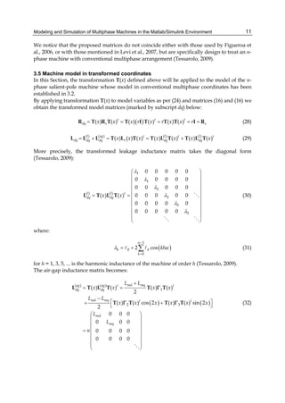
The final expression for the machine voltage equation in orthonormal coordinates is then:
dq dq dq dq dq dq dq dq
d
dt
ω= + + +v R i JL i L i e (43)
which is formally identical to the transformed voltage equation of a three-phase
synchronous machine in the rotor dq reference frame.
From (44) a simple expression for the machine electromagnetic torque can be also derived.
In fact, if we left-multiply both sides of (44) by idq
t we obtain:
t t t t t
dq dq dq dq dq dq dq dq dq dq dq dq dq
d
dt
ω= + + +i v i R i i JL i i L i i e . (44)
Using (10), (11), (24), we can write the left-hand side member of (45) as follows:
[ ]
1
0
( ) ( ) ( ) ( )
n
tt t t t
dq dq s s s s s s k k e
k
x x x x v i p
−
=
= = = = =∑i v T i T v i T T v i v (45)
where pe is the instantaneous electrical power entering machine terminals; using (14) and
(28), the term t
dq dq dqi R i can be written as:
1
2
0
n
t t t t
dq dq dq dq dq k j
k
r ri p
−
=
= = =∑i R i i i (46)](https://image.slidesharecdn.com/engineeringeducationandresearchusingmatlab-160628213608/85/Engineering-education-and_research_using_matlab-23-320.jpg)


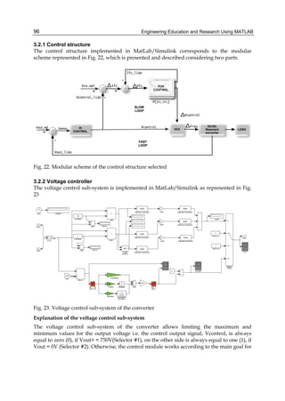
![Engineering Education and Research Using MATLAB18
a. It assigns the permutation matrices W in the stator interface blocks (Fig. 10).
Permutation matrices are selected and defined as per 3.2.1 and 3.2.2 depending on the
phase number and arrangement specified as an input;
b. It defines the variable transformation matrix T(x) as per (25) depending only on the
number of phases;
c. It builds the diagonal matrices R and inductance matrix L using respectively the phase
resistance and stator harmonic inductances (31) specified as input data;
d. It builds the constant block-diagonal matrix J as per (43) depending only on the number
of stator phases.
4.3.3 Model adaptation to different multiphase winding schemes
The adaptation of the model to implement different winding schemes can be essentially
done in the initialization stage simply by properly defining the various model matrices as
the model structure essentially remains the same. Of course, for an n-phase machine, we
shall have n pairs of terminals (one pair per phase) and thereby n of the blocks marked with
blue dashed contour in Fig. 10.
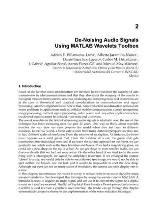
5. Examples of application
To illustrate the possible application of the method described in this Chapter, we next report
the case of a dual-star and a triple-star synchronous machines (the dual and triple three-
phase winding schemes are respectively shown in Fig. 1b and in Fig. 5a). The former (2 MW,
1200 V, 6300 rpm) is operated as a motor fed by two Load-Commutated Inverters (Castellan
et al., 2008), the latter (20 kVA, 720 V, 3000 V) is operated as a driven generator with its
stator terminals in short circuit. Both machines are simulated using the same
Matlab/Simulink model, described in Section 3, adapted to the two cases by a different
initialization of its matrices [W, C, P(x)] as reported below.
Provided that natural phase variables are arranged in vector form as follows
( )2 1 2 1 2 1 2
t
ABC A A B B C Cy y y y y y× =y , (55)
( )3 1 1 1 2 2 2 3 3 3
t
ABC A B C A B C A B Cy y y y y y y y y× =y , (56)
the permutation matrices in the two cases are given by (58) and (59) and the transformation
matrices C and P(x), used to build T(x)=P(x)C, are given by (60)-(63).
The Matlab/Simulink models used for the simulations are shown in Fig. 11 and Fig. 12,
where the yellow block represents the same model differently initialized to represent the
two different machines (shown in Fig. 13).
2 3
1 0 0 0 0 0
0 0 0 1 0 0
0 0 1 0 0 0
0 0 0 0 0 1
0 1 0 0 0 0
0 0 0 0 1 0
×
⎛ ⎞
⎜ ⎟
⎜ ⎟
⎜ ⎟−
= ⎜ ⎟
−⎜ ⎟
⎜ ⎟
⎜ ⎟
⎜ ⎟
⎝ ⎠
W , (57)](https://image.slidesharecdn.com/engineeringeducationandresearchusingmatlab-160628213608/85/Engineering-education-and_research_using_matlab-28-320.jpg)


![De-Noising Audio Signals Using MATLAB Wavelets Toolbox 27
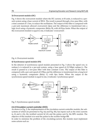
Fig. 2. Shows the process identifies the main steps in a digital audio processing system
based in Simulink software
The From Audio Device block buffers the data from the audio device by means of using the
process illustrated by Figure 2. We selected the block MATLAB Simulink audio and
multimedia file block in order to save the audio acquired by a given time. Figure 3 shows
the From Audio Device GUI, where we selected a 5 second queue period. At the start of the
simulation, the audio device writes input data to a buffer. When the buffer is full, the From
Audio Device block writes the contents of the buffer to the queue. The size of this queue can
be specified in the queue duration (seconds) parameter. As the audio device appends audio
data to the bottom of the queue, the From Audio Device block pulls data from the top of the
queue to fill the Simulink frame. We used this file to make our de-noise method using
wavelets.
Fig. 3. Shows block diagram of audio acquire
We used the wavread function. It loads a: WAVE file specified by the string filename,
returning the sampled data in y. If the filename does not include an extension, wavread
appends a .wav extension. Example code is: [x,Fs,nbits]= wavread(‘filename’) where the function
returns the filename with the number of bits per sample (nbits).
[x,Fs,nbits]= wavread ('voice');
y = awgn(x,10,'measured');
For example, wavwrite(y,Fs,’filename’) writes the data stored in the variable y to a WAVE file
called ‘filename’. The data have a sample rate, Fs, in Hz and is assumed 16-bit.
wavwrite(y,Fs,'noisyvoice')
wavwrite(xd,Fs,'voice5')
3. Basic noise theory
Noise is defined as an unwanted signal that interferes with the communication or
measurement of another signal. A noise itself is an information-bearing signal that conveys
information regarding the sources of the noise and the environment in which it propagates.](https://image.slidesharecdn.com/engineeringeducationandresearchusingmatlab-160628213608/85/Engineering-education-and_research_using_matlab-37-320.jpg)
![Engineering Education and Research Using MATLAB28
There are many types and sources of noise or distortions and they include:
1. Electronic noise such as thermal noise and shot noise,
2. Acoustic noise emanating from moving, vibrating or colliding sources such as revolving
machines, moving vehicles, keyboard clicks, wind and rain,
3. Electromagnetic noise that can interfere with the transmission and reception of voice,
image and data over the radio-frequency spectrum,
4. Electrostatic noise generated by the presence of a voltage,
5. Communication channel distortion and fading and
6. Quantization noise and lost data packets due to network congestion.
Signal distortion is the term often used to describe a systematic undesirable change in a
signal and refers to changes in a signal from the non-ideal characteristics of the
communication channel, signal fading reverberations, echo, and multipath reflections and
missing samples. Depending on its frequency, spectrum or time characteristics, a noise
process is further classified into several categories:
1. White noise: purely random noise has an impulse autocorrelation function and a flat
power spectrum. White noise theoretically contains all frequencies in equal power.
2. Band-limited white noise: Similar to white noise, this is a noise with a flat power spectrum
and a limited bandwidth that usually covers the limited spectrum of the device or the
signal of interest. The autocorrelation of this noise is sinc-shaped.
3. Narrowband noise: It is a noise process with a narrow bandwidth such as 50/60 Hz from
the electricity supply.
4. Coloured noise: It is non-white noise or any wideband noise whose spectrum has a non-
flat shape. Examples are pink noise, brown noise and autoregressive noise.
5. Impulsive noise: Consists of short-duration pulses of random amplitude, time of
occurrence and duration.
6. Transient noise pulses: Consist of relatively long duration noise pulses such as clicks,
burst noise etc.
3.1 Signal to noise ratio
The signal-to-noise ratio (SNR) is commonly used to assess the effect of noise on a signal.
This measurement is based on an additive noise model, where the quantized signal xq[n] is
a superposition of the unquantized, undistorted signal x[n] and the additive quantization
error e[n]. The ratio between the signal powers of x[n] and e[n] defines the SNR. To capture
the wide range of potential SNR values and to consider the logarithmic perception of
loudness in humans, SNR generally given in a logarithmic scale, in decibels (dB)
2
10 2
10 * log ,x
dB
e
SNR
σ
σ
= (1)
Where, σ2x and σ2
e are the powers of x[n], and e[n], respectively. Specifically for the
assessment of quantization noise, SNR is often labeled as the signal to quantization-noise
ratio (SQNR).
3.2 White noise
Shown in Figure 4, white noise is defined as an uncorrelated random noise process with
equal power at all frequencies. Random noise has the same power at all frequencies in the
range of ∞ it would necessarily need to have infinite power, and it is therefore an only a](https://image.slidesharecdn.com/engineeringeducationandresearchusingmatlab-160628213608/85/Engineering-education-and_research_using_matlab-38-320.jpg)


![De-Noising Audio Signals Using MATLAB Wavelets Toolbox 37
Figure 13 shows the plot of a signal after its processing method using Coiflet 5.
Amplitude
1
0
-1
0.9 0.92 0.94 0.96 0.98 1
Time (s)
0.9 0.902 0.904 0.906 0.908
Time (s)
Amplitude
1
0
-1
Fig. 13. Shows signal after processing method of de-noise using Coiflet 5
Evaluation of the resultant waveform xd presented in Figure 14 is compared with the
original sine function x form Figure 11 gives numbers higher than 99% as presented in
Figure 13. These results support the reliability of the proposed method for de-noising.
6. Audio signal example
As it has been described in section 2.1, to obtain an audio signal, we select the audio block
and we connect it to the multimedia file block. This information is saved in a user-specified
file with extension .wav and then we use the program to extract this information and
process it with wavelets coif5, db9 and db10. Figure 14 shows the original audio signal, audio
signal with noise and the recovered signal using the wavelet coif5. Figure 15 shows the best
correlation using the above wavelets.
Amplitude
1
0
-1
0 0.5 1 1.5 2 2.5 3 3.5 4 4.5 5
Time (s)
Original Signal
Amplitude
2
0
-2
0 0.5 1 1.5 2 2.5 3 3.5 4 4.5 5
Time (s)
Signal With Noise
Amplitude
2
0
-2
0 0.5 1 1.5 2 2.5 3 3.5 4 4.5 5
Time (s)
Signal Denoise
Fig. 14. Shows original audio signal, audio signal with noise and the recovered signal
To make the signal processing we use the next code:
clc,close all,clear all
k = 0:9.0703e-005:5;
w=500*pi;
h=w.*k;
[x,Fs,nbits]= wavread ('voice');
y = awgn(x,10,'measured'); % Add white Gaussian noise.](https://image.slidesharecdn.com/engineeringeducationandresearchusingmatlab-160628213608/85/Engineering-education-and_research_using_matlab-47-320.jpg)


![De-Noising Audio Signals Using MATLAB Wavelets Toolbox 41
In our case, a slider is coupled to an edit text component so that: The edit text displays the
current value of the slider. The user can enter a value into the edit text box and cause the
slider to update to that value. Both components update the appropriate model parameters
when activated by the user. Our slider is called AWGN (average white generator noise) and
it is from 0 to 10 SNR.
function complete_OpeningFcn(hObject, eventdata, handles, varargin)
% Choose default command line output for example5
handles.output = hObject;
clc
% initalize error count and use edit1 object's userdata to store it.
data.number_errors = 0;
set(handles.edit1,'UserData',data)
% Update handles structure
guidata(hObject, handles);
% --- Executes on slider movement.
function slider1_Callback(hObject, eventdata, handles)
set(handles.edit1,'String',...
num2str(get(hObject,'Value')));
% --- Executes during object creation, after setting all properties.
function slider1_CreateFcn(hObject, eventdata, handles)
function edit1_Callback(hObject, eventdata, handles)
val = str2double(get(hObject,'String'));
% Determine whether val is a number between 0 and 10.
if isnumeric(val) && length(val)==10 && ...
val >= get(handles.slider1,'min') && ...
val <= get(handles.slider1,'max')
set(handles.slider1,'Value',val);
else
% Retrieve and increment the error count.
% Error count is in the edit text UserData,
% so we already have its handle.
data = get(hObject,'UserData');
data.number_errors = data.number_errors+1;
% Save the changes.
set(hObject,'UserData',data);
% Display new total.
set(hObject,'String',...
['You have entered an invalid entry ',...
num2str(data.number_errors),' times.']);
% Restore focus to the edit text box after error
uicontrol(hObject)
end
% --- Executes during object creation, after setting all properties.
function edit1_CreateFcn(hObject, eventdata, handles)
if ispc && isequal(get(hObject,'BackgroundColor'),
get(0,'defaultUicontrolBackgroundColor'))
set(hObject,'BackgroundColor','white');
end](https://image.slidesharecdn.com/engineeringeducationandresearchusingmatlab-160628213608/85/Engineering-education-and_research_using_matlab-51-320.jpg)
![Engineering Education and Research Using MATLAB42
In the case of the pushbutton 1 that is called sine, and if it only shows sine signal and signal
with noise, it needs to be programmed as follow
% --- Executes on button press in pushbutton1.
function pushbutton1_Callback(hObject, eventdata, handles)
k =(0:9.0703e-005:5);
w=500*pi;
h=w.*k;
x = sin(h);
f=get(handles.slider1,'Value');
y = awgn(x,f,'measured');
D=crosscorr(x,y);
z=-20:1:20;
plot(handles.axes1,k,x)
plot(handles.axes2,k,y)
plot(handles.axes3,z,D)
For programming, push button 2, called de-noise sine, this button performs all the
processing method, which was described previously. It is necessary to write all this code
% --- Executes on button press in pushbutton2.
function pushbutton2_Callback(hObject, eventdata, handles)
menu= get(handles.popupmenu1,'Value');
switch menu
case 1 %case 1: coiflet 5
·% example3 code
k =(0:9.0703e-005:5);
w=500*pi;
h=w.*k;
x = sin(h);
f=get(handles.slider1,'Value');
y = awgn(x,f,'measured');
wname = 'coif5'; lev = 10; % wavelet that need to change!
tree = wpdec(y,lev,wname);
det1 = wpcoef(tree,2);
sigma = median(abs(det1))/0.6745;
alpha = 2;
thr =wpbmpen(tree,sigma,alpha);
keepapp = 1;
xd = wpdencmp(tree,'s','nobest',thr,keepapp);
D=crosscorr(x,xd);
z=-20:1:20;
plot(handles.axes1,k,x)
plot(handles.axes2,k,y)
plot(handles.axes3,k,xd)
set(gca,'XLim',[ 0.2, 0.24], ...
'YLim',[-1 1]);
plot(handles.axes4,z,D)
case 2 %case2 Daubechies 10](https://image.slidesharecdn.com/engineeringeducationandresearchusingmatlab-160628213608/85/Engineering-education-and_research_using_matlab-52-320.jpg)
![De-Noising Audio Signals Using MATLAB Wavelets Toolbox 43
·% example3 code
case 3 %Case 3: Daubechies 9
·% example3 code
End
For programing push button 3, called de-noise audio, this button performs all processing
method, which was described previously. It is necessary to write all this code
% --- Executes on button press in pushbutton3.
function pushbutton3_Callback(hObject, eventdata, handles)
menu= get(handles.popupmenu1,'Value');
switch menu
case 1 %case 1: Coiflet 5
·% example4 code
k = 0:9.0703e-005:5;
w=500*pi;
h=w.*k;
[x,Fs,nbits]= wavread ('voice');
f=get(handles.slider1,'Value');
y = awgn(x,f,'measured');
wavwrite(y,Fs,'noisyvoice')
wname = 'coif5'; lev = 10;
tree = wpdec(y,lev,wname);
det1 = wpcoef(tree,2);
sigma = median(abs(det1))/0.6745;
alpha = 2;
thr =wpbmpen(tree,sigma,alpha);
keepapp = 1;
xd = wpdencmp(tree,'s','nobest',thr,keepapp);
D=crosscorr(x,xd);
z=-20:1:20;
plot(handles.axes1,k,x)
plot(handles.axes2,k,y)
plot(handles.axes3,k,xd)
plot(handles.axes4,z,D)
case 2 %case2 Daubechies 10
·% example4 code
case 3 %Case 3: Daubechies 9
·% example4 code
end
For programing push button 4 called exit
% --- Executes on button press in pushbutton4.
function pushbutton3_Callback(hObject, eventdata, handles)
close all
Figure 18 (left) shows AWGN 1, and it plots original signal, in this case sine, and signal with
noise, cross correlation between them. Figure 18 (right) shows sine after de-noise and cross
correlation between the original signal and the de-noised.](https://image.slidesharecdn.com/engineeringeducationandresearchusingmatlab-160628213608/85/Engineering-education-and_research_using_matlab-53-320.jpg)


![Engineering Education and Research Using MATLAB48
signal
wavelet
C=0.2247
C=0.0102
signal
wavelet
signal
wavelet
signal
wavelet
Fig. A. Shows recipe for creating a CWT
Appendix B: User Interface MATLAB code
In this appendix, it shows the complete code to develop the GUI using the GUIDE of
MATLAB, and develops it as an example using a sine wave signal, which is added a certain
level of noise and signal is shown graphically also recovered as the ratio correlation between
the original signal and recovered signal.
function varargout = complete(varargin)
% Begin initialization code - DO NOT EDIT
gui_Singleton = 1;
gui_State = struct('gui_Name', mfilename, ...
'gui_Singleton', gui_Singleton, ...
'gui_OpeningFcn', @complete_OpeningFcn, ...
'gui_OutputFcn', @complete_OutputFcn, ...
'gui_LayoutFcn', [] , ...
'gui_Callback', []);
if nargin && ischar(varargin{1})
gui_State.gui_Callback = str2func(varargin{1});
end
if nargout
[varargout{1:nargout}] = gui_mainfcn(gui_State, varargin{:});
else
gui_mainfcn(gui_State, varargin{:});
end
% End initialization code - DO NOT EDIT
% --- Executes just before complete is made visible.
function complete_OpeningFcn(hObject, eventdata, handles, varargin)
handles.output = hObject;
clc
% Initalize error count and use edittext1 object's userdata to store it.](https://image.slidesharecdn.com/engineeringeducationandresearchusingmatlab-160628213608/85/Engineering-education-and_research_using_matlab-58-320.jpg)
![De-Noising Audio Signals Using MATLAB Wavelets Toolbox 49
data.number_errors = 0;
set(handles.edit1,'UserData',data)
% Update handles structure
guidata(hObject, handles);
% --- Outputs from this function are returned to the command line.
function varargout = complete_OutputFcn(hObject, eventdata, handles)
% Get default command line output from handles structure
varargout{1} = handles.output;
% --- Executes on button press in pushbutton1.
function pushbutton1_Callback(hObject, eventdata, handles)
k =(0:9.0703e-005:5);
w=500*pi;
h=w.*k;
x = sin(h);
f=get(handles.slider1,'Value');
y = awgn(x,f,'measured');
D=crosscorr(x,y);
z=-20:1:20;
plot(handles.axes1,k,x)
plot(handles.axes2,k,y)
plot(handles.axes4,z,D)
% --- Executes on button press in pushbutton2.
function pushbutton2_Callback(hObject, eventdata, handles)
menu= get(handles.popupmenu1,'Value');
switch menu
case 1 %case 1: Coiflet 5
k =(0:9.0703e-005:5);
w=500*pi;
h=w.*k;
x = sin(h);
f=get(handles.slider1,'Value');
y = awgn(x,f,'measured');
wname = 'coif5'; lev = 10;
tree = wpdec(y,lev,wname);
det1 = wpcoef(tree,2);
sigma = median(abs(det1))/0.6745;
alpha = 2;
thr =wpbmpen(tree,sigma,alpha);
keepapp = 1;
xd = wpdencmp(tree,'s','nobest',thr,keepapp);
D=crosscorr(x,xd);
z=-20:1:20;
plot(handles.axes1,k,x)
plot(handles.axes2,k,y)
plot(handles.axes3,k,xd)
set(gca,'XLim',[ 0.2, 0.24], ...
'YLim',[-1 1]);](https://image.slidesharecdn.com/engineeringeducationandresearchusingmatlab-160628213608/85/Engineering-education-and_research_using_matlab-59-320.jpg)
![Engineering Education and Research Using MATLAB50
plot(handles.axes4,z,D)
case 2 %Case2 Daubechies 10
k =(0:9.0703e-005:5);
w=500*pi;
h=w.*k;
x = sin(h);
f=get(handles.slider1,'Value');
y = awgn(x,f,'measured');
wname = 'db10'; lev = 10;
tree = wpdec(y,lev,wname);
det1 = wpcoef(tree,2);
sigma = median(abs(det1))/0.6745;
alpha = 2;
thr =wpbmpen(tree,sigma,alpha);
keepapp = 1;
xd = wpdencmp(tree,'s','nobest',thr,keepapp);
D=crosscorr(x,xd);
z=-20:1:20;
plot(handles.axes1,k,x)
plot(handles.axes2,k,y)
plot(handles.axes3,k,xd)
set(gca,'XLim',[ 0.2, 0.24], ...
'YLim',[-1.1 1.1]);
plot(handles.axes4,z,D)
case 3 %Case 3: Daubechies 9
k =(0:9.0703e-005:5);
w=500*pi;
h=w.*k;
x = sin(h);
f=get(handles.slider1,'Value');
y = awgn(x,f,'measured');
wname = 'db9'; lev = 10;
tree = wpdec(y,lev,wname);
det1 = wpcoef(tree,2);
sigma = median(abs(det1))/0.6745;
alpha = 2;
thr =wpbmpen(tree,sigma,alpha);
keepapp = 1;
xd = wpdencmp(tree,'s','nobest',thr,keepapp);
D=crosscorr(x,xd);
z=-20:1:20;
plot(handles.axes1,k,x)
plot(handles.axes2,k,y)
plot(handles.axes3,k,xd)
plot(handles.axes4,z,D)
end](https://image.slidesharecdn.com/engineeringeducationandresearchusingmatlab-160628213608/85/Engineering-education-and_research_using_matlab-60-320.jpg)
![De-Noising Audio Signals Using MATLAB Wavelets Toolbox 51
% --- Executes on button press in pushbutton3.
function pushbutton3_Callback(hObject, eventdata, handles)
menu= get(handles.popupmenu1,'Value');
switch menu
case 1 %case 1: coiflet 5
k = 0:9.0703e-005:5;
w=500*pi;
h=w.*k;
[x,Fs,nbits]= wavread ('voice');
f=gethandles.slider1,'Value');
y = awgn(x,f,'measured');
wavwrite(y,Fs,'noisyvoice')
wname = 'coif5'; lev = 10;
tree = wpdec(y,lev,wname);
det1 = wpcoef(tree,2);
sigma = median(abs(det1))/0.6745;
alpha = 2;
thr =wpbmpen(tree,sigma,alpha);
keepapp = 1;
xd = wpdencmp(tree,'s','nobest',thr,keepapp);
D=crosscorr(x,xd);
z=-20:1:20;
plot(handles.axes1,k,x)
plot(handles.axes2,k,y)
plot(handles.axes3,k,xd)
plot(handles.axes4,z,D)
case 2 %case 2 Daubechies 10
k = 0:9.0703e-005:5;
w=500*pi;
h=w.*k;
[x,Fs,nbits]= wavread ('voice');
f=get(handles.slider1,'Value');
y = awgn(x,f,'measured');
wavwrite(y,Fs,'noisyvoice')
wname = 'db10'; lev = 10;
tree = wpdec(y,lev,wname);
det1 = wpcoef(tree,2);
sigma = median(abs(det1))/0.6745;
alpha = 2;
thr =wpbmpen(tree,sigma,alpha);
keepapp = 1;
xd = wpdencmp(tree,'s','nobest',thr,keepapp);
D=crosscorr(x,xd);
z=-20:1:20;
plot(handles.axes1,k,x)
plot(handles.axes2,k,y)
plot(handles.axes3,k,xd)](https://image.slidesharecdn.com/engineeringeducationandresearchusingmatlab-160628213608/85/Engineering-education-and_research_using_matlab-61-320.jpg)
![Engineering Education and Research Using MATLAB52
plot(handles.axes4,z,D)
case 3 %Case 3: Daubechies 9
k = 0:9.0703e-005:5;
w=500*pi;
h=w.*k;
[x,Fs,nbits]= wavread ('voice');
f=get(handles.slider1,'Value');
y = awgn(x,f,'measured');
wavwrite(y,Fs,'noisyvoice')
wname = 'db9'; lev = 10;
tree = wpdec(y,lev,wname);
det1 = wpcoef(tree,2);
sigma = median(abs(det1))/0.6745;
alpha = 2;
thr =wpbmpen(tree,sigma,alpha);
keepapp = 1;
xd = wpdencmp(tree,'s','nobest',thr,keepapp);
D=crosscorr(x,xd);
z=-20:1:20;
plot(handles.axes1,k,x)
plot(handles.axes2,k,y)
plot(handles.axes3,k,xd)
plot(handles.axes4,z,D)
end
% --- Executes on slider movement.
function slider1_Callback(hObject, eventdata, handles)
set(handles.edit1,'String',...
num2str(get(hObject,'Value')));
% --- Executes during object creation, after setting all properties.
function slider1_CreateFcn(hObject, eventdata, handles)
if isequal(get(hObject,'BackgroundColor'), get(0,'defaultUicontrolBackgroundColor'))
set(hObject,'BackgroundColor',[.9 .9 .9]);
end
function edit1_Callback(hObject, eventdata, handles)
val = str2double(get(hObject,'String'));
% Determine whether val is a number between 0 and 1.
if isnumeric(val) && length(val)==10 && ...
val >= get(handles.slider1,'min') && ...
val <= get(handles.slider1,'max')
set(handles.slider1,'Value',val);
else
% Retrieve and increment the error count.
% Error count is in the edit text UserData,
% so we already have its handle.
data = get(hObject,'UserData');
data.number_errors = data.number_errors+10;](https://image.slidesharecdn.com/engineeringeducationandresearchusingmatlab-160628213608/85/Engineering-education-and_research_using_matlab-62-320.jpg)
![De-Noising Audio Signals Using MATLAB Wavelets Toolbox 53
% Save the changes.
set(hObject,'UserData',data);
% Display new total.
set(hObject,'String',...
['You have entered an invalid entry ',...
num2str(data.number_errors),' times.']);
% Restore focus to the edit text box after error
uicontrol(hObject)
end
% --- Executes during object creation, after setting all properties.
function edit1_CreateFcn(hObject, eventdata, handles)
if ispc && isequal(get(hObject,'BackgroundColor'),
get(0,'defaultUicontrolBackgroundColor'))
set(hObject,'BackgroundColor','white');
end
% --- Executes on selection change in popupmenu1.
function popupmenu1_Callback(hObject, eventdata, handles)
% --- Executes during object creation, after setting all properties.
function popupmenu1_CreateFcn(hObject, eventdata, handles)
if ispc && isequal(get(hObject,'BackgroundColor'),
get(0,'defaultUicontrolBackgroundColor'))
set(hObject,'BackgroundColor','white');
end
% --- Executes on button press in pushbutton4.
function pushbutton4_Callback(hObject, eventdata, handles)
close all
10. References
Abbate A, Decusatis C. M, Das P. K. (2002). Wavelets and subbands: fundamentals and
applications, ISBN 0-8176-4136-X, Birkhauser, Boston, USA.
Bahoura M & Rouat J, (2006). Wavelet speech enhancement based on time–scale adaptation,
Speech Communication, Vol. 48, No. 12, pp: 1620-1637. ISSN: 0167-6393.
Davis, G, M, (2002). ‘Noise Reduction in Speech Applications, CRC Press LLC, ISBN 0-8493-
0949-2, USA.
Dong E & Pu X. (2008). Speech denoising based on perceptual weighting filter, Proceedings
of 9th IEE International Conference on Signal Processing, pp: 705-708, October 26-
29, Beijing. Print ISBN: 978-1-4244-2178-7.
Gold, B. & Morgan, N. (1999) Speech and audio signal processing: processing and
perception of apeech, and music, John Wiley & Sons, INC., ISBN: 0-471-35154-7,
New York, USA.
Johnson M. T, Yuan X and Ren Y, (2007). Speech Signal Enhancement through Adaptive
Wavelet Thresholding, Speech Communications, Vol. 49, No. 2, pp: 123-133, ISSN:
0167-6393.
Képesia M & Weruaga L. (2006). Adaptive chirp-based time–frequency analysis of speech
signals, Speech Communication, Vol. 48, No. 5, pp: 474-492. ISSN: 0167-6393.](https://image.slidesharecdn.com/engineeringeducationandresearchusingmatlab-160628213608/85/Engineering-education-and_research_using_matlab-63-320.jpg)


![Engineering Education and Research Using MATLAB60
Target application. Installing the kernel configures it to start running in the background
each time you start your computer. The kernel installation is done in the workspace by
typing:
>> rtwintgt – install
You can also use the command rtwintgt -setup to install the kernel. The MATLAB
Command Window displays one of these messages:
>> You are going to install the Real-Time Windows Target kernel.
Do you want to proceed? [y] :
or:
>> There is a different version of the Real-Time Windows Target kernel installed.
Do you want to update to the current version? [y] :
Type y to continue installing the kernel, or n to cancel installation without making any
change. If you type y, the MATLAB environment installs the kernel and displays the
message:
>> The Real-Time Windows Target kernel has been successfully installed.
If a message appears asking you to restart your computer, do so before attempting to use the
kernel, or your Real-Time Windows Target model will not run correctly. After installing the
kernel, verify that it was correctly installed by typing:
>> rtwho
The MATLAB Command Window should display a message that shows the kernel version
number, followed by performance, timeslice, and other information.
>>Real Time Windows Target version 1.00 (C) The MathWorks, Inc. 1994-2010
Running on Multiprocessor APIC computer
MATLAB performance = 98.5%
Kernel timeslice period = 0.999 ms
Matlab specifies the performance of the running application on the actual PC and the used
sampling time. It is desirable to execute your applications near 100% performance, is not
recommended to use values of performance near to 50% because the switching execution
time will decrease in the real time windows target in order to attend other programs in the
Operative system.
Once the kernel is installed, you can leave it installed. The kernel remains idle after you
have installed it, which allows the Windows operating system to control the execution of
any standard Windows based application, including Internet browsers, word processors, the
MATLAB environment, and so on. The kernel becomes active when you begin execution of
your model, and becomes idle again after model execution completes.
The Real-Time Windows Target requires a C compiler which is not included in the
installation in MATLAB. To choose the compiler to use it is necessary to type the following
command in the workspace:
>> mex –setup](https://image.slidesharecdn.com/engineeringeducationandresearchusingmatlab-160628213608/85/Engineering-education-and_research_using_matlab-70-320.jpg)
![A Matlab® Approach for Implementing Control Algorithms in Real-Time: RTWT 61
The following dialog will appear:
>> Would you like mex to locate installed compilers [y]/n? y
Select a compiler:
[1] Intel Visual Fortran 9.1 (with Microsoft Visual C++ 2005 linker) in
C:Program FilesIntelCompilerFortran9.1
[2] Lcc-win32 C 2.4.1 in C:PROGRA~1MATLABR2007bsyslcc
[3] Microsoft Visual C++ 2005 in
C:Program FilesMicrosoft Visual Studio 8
[0] None
After you choose your compiler for instance, Compiler: 2, the following dialog will appear:
>> Please verify your choices:
Compiler: Lcc-win32 C 2.4.1
Location: C:PROGRA~1MATLABR2007bsyslcc
>> Are these correct?([y]/n): y
Done . . .
After you confirm your choice typing y the process finish it. You can use any PC-compatible
computer that runs Microsoft® Windows XP 32-bit, or Microsoft Windows Vista ™ 32-bit.
Your computer can be a desktop, laptop, or notebook PC.
4.5 Hardware I/O boards
Real-Time Windows Target applications use standard and inexpensive I/O boards for PC-
compatible computers. When running your models in real time, RTWT captures the
sampled data from one or more input channels, uses the data as inputs to your block
diagram model, immediately processes the data, and sends it back to the outside world
through an output channel on your I/O board.
Real-Time Windows Target software provides a custom Simulink block library. The I/O
driver block library contains universal drivers for supported I/O boards. These universal
blocks are configured to operate with the library of supported drivers. This allows easy
location of driver blocks and easy configuration of I/O boards. You drag and drop an
universal I/O driver block from the I/O library the same way as you would from a standard
Simulink block library. And you connect an I/O driver block to your model just as you
would connect any standard Simulink block.
You create a real-time application in the same way as you create any other Simulink model,
by using standard blocks and C-code S-functions. You can add input and output devices to
your Simulink model by using the I/O driver blocks from the rtwinlib library provided
with the Real-Time Windows Target software. This library contains the blocks depicted in
figure 1.
The Real-Time Windows Target software provides driver blocks for more than 200 I/O
boards. These driver blocks connect the physical world to your real-time application:
• Sensors and actuators are connected to I/O boards.
• I/O boards convert voltages to numerical values and numerical values to voltages.
• Numerical values are read from or written to I/O boards by the I/O drivers.](https://image.slidesharecdn.com/engineeringeducationandresearchusingmatlab-160628213608/85/Engineering-education-and_research_using_matlab-71-320.jpg)


![Engineering Education and Research Using MATLAB64
are several options available when we press the ‘Browse’ button, however we must select
‘rtwin.tlc’ which is the Real-Time Windows Target. The language can be selected as C or
C++, we choose C language by default. We accept these changes and return to our model in
Simulink. At this point we can choose the simulation as external mode, as depicted in Figure
5. Remember to save your model by pressing the keys ‘ctrl+S’
Fig. 5. Configuring the simulation in External mode
Configuring the analog input and output
After our simulation parameters has been configured, then we can continue with the process
interfacing. By double clicking in the analog output block in our Simulink model, the
configuration window will appear as depicted in Figure 6. In this window we must select
our hardware board, in this case the National Instruments acquisition board DAQCard-
6024E. The sampling time is selected as ‘Ts’, which can be previously defined in the
workspace as Ts=0.002. In this step also the output range can be configured, which is in our
case from -10 V to 10 V. Some initial and final values can be established at this point, for the
cases when we need that the DAQ board remains with some value after the simulation
stops. It is possible to test our hardware to verify that there are not communication
problems between Simulink and our external hardware. By pressing the ‘Board Setup’ button
a new window will appear, and by pressing the ‘Test’ Button we can test all the inputs and
outputs available in our board. To configure the analog input the same procedure must be
followed, the only difference is that you’ll not find the ‘initial’ and ‘final’ value parameters
available in the analog output.
Discrete PID configuration
For this application we have tuned the parameters of a PID controller by means of the KCR
algorithm (Hernandez et al, 2010); this procedure will not be described here, because our
interest is to present how to use the Real-Time Windows Target toolbox.
The discrete PID controller used in this work can be found in the: SimPowerSystems/Extra
Library/Discrete Control Blocks/Discrete PID Controller (Figure 7). This block implements
a discrete PID controller, where the Kp, Ki, Kd and sampling time Ts parameters can be
configured. There are also some other options available, e.g. the time constant for the
derivative action or the constraints in the output, which have been selected as 1000 and
[-1 1] respectively.
Scope configuration to display and save data
Until now, the simulation parameters, PID and I/O have been configured; nevertheless,
another important issue to solve is how to save the data on our hard disk. By double clicking](https://image.slidesharecdn.com/engineeringeducationandresearchusingmatlab-160628213608/85/Engineering-education-and_research_using_matlab-74-320.jpg)


![Engineering Education and Research Using MATLAB68
0 0.1 0.2 0.3 0.4 0.5 0.6 0.7 0.8 0.9 1
-2
-1
0
1
2
Time [sec]
Voltage[V]
Reference
Out openloop
Out closedloop
0 0.1 0.2 0.3 0.4 0.5 0.6 0.7 0.8 0.9 1
-2
-1
0
1
2
Time [sec]
Voltage[V]
Ctrl effort
(a)
0 5 10 15 20 25 30 35 40 45 50
-15
-10
-5
0
5
10
Bode characteristic Closed and Open loop
Magnitude[dB]
Open loop
Closed loop
0 5 10 15 20 25 30 35 40 45 50
-100
-50
0
50
100
150
Phase[Degree]
Frequency [Hz]
(b)
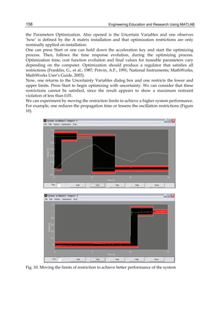
Fig. 12. Open and Closed loop characteristics. a) Performance in time. b) Performance in
frequency](https://image.slidesharecdn.com/engineeringeducationandresearchusingmatlab-160628213608/85/Engineering-education-and_research_using_matlab-78-320.jpg)


![MatLab in Model-Based Design for Power Electronics Systems 83
resistance decays linearly from 0.1229 to zero during the time interval of t0 to t1, being equal
to 1MΩ during the time interval between zero and t0, and again equal to 1MΩ when either
some starter time has elapsed or if the speed exceeds 30π radmec/s.
Fig. 11. Starter-rheostat module
2.3 Simulation results
The simulation results are obtained considering the following parameters and conditions:
integration method; ode23tb [stiff/TR-BDF2], step variable with a maximum value of 2e-4;
absolute and relative tolerances of 10e-3; reference speed of 30π radmec/s and interval of
time simulation of 0-10 seconds. The variations of the angles of the inverter and rectifier
bridges are respectively: 90º 150ºIα< < and 5º 90ºRα< < .
2.3.1 Electromagnetic and mechanical torques
The electromagnetic torque is measured directly from the block model of the three-phase
asynchronous machine selected in the library of MatLab/Simulink software. The S.I. unit
parameter is selected. All the stator and rotor quantities are referred to in the rotor reference
frame (qd frame). Considering an electrical system with these conditions, the electromagnetic
torque is given by Eq. 1. In this equation p corresponds to the number of pole pairs, dsϕ and](https://image.slidesharecdn.com/engineeringeducationandresearchusingmatlab-160628213608/85/Engineering-education-and_research_using_matlab-93-320.jpg)


![Engineering Education and Research Using MATLAB120
( )
( )( )( )
( )( )( )
2 2
2 2
1 1.998 1 1.994 1
0.8116 1.676 0.7128 1.837 0.8782
z z z z z
NTF z
z z z z z
− − ⋅ + − ⋅ +
=
− − ⋅ + − ⋅ +
(1)
It is possible to implement such transfer function in many different ways. Based on
additional requirements such as small power supply consumption and stability under
different signal conditions, we selected feed-forward architecture with only one feedback,
presented in Fig. 2. It has a one-bit internal quantizer, a one bit internal D/A converter, and
a feed-forward structure with one feedback coefficient 1refb .
Coefficients 0α , 0δ , 1,2β , 1,2γ , 1,2η and 1,2λ from (2) are related in a complex way to the
feedback and feed-forward coefficients represented by vectors a, g, b, c of the circuit shown
on Fig.2. They can be calculated using function: [a,g,b,c] = realizeNTF(NTF, FORM, STF)
from package “delsig” (Schreier, 2009), where [a,g,b,c] are vectors of coefficients from Fig.
2. The NTF (noise transfer function) is given by (1); STF (signal transfer function) STF=1 and
FORM refers to the form of the architecture and are selected as the feed-forward structure.
Fig. 1. Noise transfer function plot of (1). Upper plot: |NTF(z)| from 0 to 0.5*fs. Lower plot:
|NTF(z)| pass-band detail
Input signal is added to the first integrator through coefficient 1inb and to the quantizer input
through coefficient b6. The state variables ( )1x z through ( )5x z are the outputs of discrete
time integrators. The coefficients g1 and g2 determine the positions of complex conjugate
poles, while weighted state variables with weights 1a through 5a that are added together,
with weighted input signal ( 6b ), contribute to the signal at the input of one bit internal
quantizer. In this way, a complex conjugate zeros of (1) are formed. A linear model is
formed if the internal quantizer is replaced by an adder that adds signal ( )6x z with
quantization noise ( )Q z and use gain 1k = . One can determine the poles and the zeroes of](https://image.slidesharecdn.com/engineeringeducationandresearchusingmatlab-160628213608/85/Engineering-education-and_research_using_matlab-130-320.jpg)
![Mixed-Signal Circuits Modelling and Simulations Using Matlab 121
noise transfer function ( )xNTF z of the block diagram on Fig. 2. using symbolic and
optimization toolbox of the Matlab and some “hand” written state space equations. The
result is given in (2).
( )
( )
( )
( )( )( )
( )( )( )
2 2
0 1 1 2 2
2 2
0 1 1 2 2
C
z z z z zV z
NTF z
Q z z z z z z
α β γ β γ
δ η λ η λ
− − + − +
= =
− − + − +
(2)
Fig. 2. Block diagram of a fifth order Σ-Δ modulator with feed-forward architecture. State
variables ( )ix z are outputs of the integrators
All coefficients are calculated by assuming the linear model of the Σ-Δ modulator. Of course,
coefficients obtained in this way do not produce appropriately scaled state variables of the
modulators’ loop transfer function and further scaling steps will be needed; these are
explained in the following subsections. For NTF(z) from (1), STF(z)=1, and for the selected
feed-forward architecture the coefficients are (3):
[ ]
[ ]
[ ]
[ ]
1.431.35 0.98 0.53 0.067
0.0090 0.0633
0.23 0 0 0 0 0.5
= 0.23 0.33 0.25 0.18 0.099
T
T
T
T
=
=
=
a
g
b
c
(3)
To check the validity of the synthesis algorithm, we can calculate the spectrum of the linear
model of the modulators’ bit-stream V(n). The state space description of the linear model of
the circuit from Fig. 2 is defined in (4).
( ) ( ) ( )
( ) ( ) ( )
( ) ( ) ( ) ( )
6
1
T
in
in in ref ref
y n n b v n
v n k y n q n
x n n v n b v n v
= +
= +
= + +
a x
Ax b
(4)](https://image.slidesharecdn.com/engineeringeducationandresearchusingmatlab-160628213608/85/Engineering-education-and_research_using_matlab-131-320.jpg)


![Mixed-Signal Circuits Modelling and Simulations Using Matlab 125
“unlimited”, while the output data type is set to “Inherited”, and therefore the data
type is double.
Fig. 8. The Product symbol
• Relay: The comparator can be in the simplest way modelled as a relay. The parameters
that must be set are the following: Switch on point (VH), Switch off point (VL), Output
when on (1), Output when off (-1), Enabled zero crossing, and sample time (-
1=Inherited). The switching levels are defined in the main Matlab m-file. In our case, a
small hysteresis is built-in and taken into consideration as follows: VH=1mV and VL=-
1mV. The output levels (BS) are set to ±1.
Fig. 9. The Relay symbol
• DT integrator: The last element used in the simplified model of our example
modulator is a discrete time integrator shown in Fig. 10. In the ideal and simplest case,
it can be modelled by a discrete transfer function with pole at z=1, followed by a Zero-
Order-Hold block. The transfer function coefficients are defined in the “Main” pane of
the parameter settings, with Numerator coefficients set to [1] and Denominator
coefficients set to [1 -1]. In addition, the Sample time is set to Ts, and is defined in the
main Matlab routine before running the Simulink simulation. The State attributes in this
case are unimportant and default settings can be accepted. All five integrators are
equivalent for the ideal Simulink model.
Fig. 10. Discrete time integrator model used in example modulator
• Top level: To run the simulation and to store some results, a top-level scheme is needed
that consists of system to be simulated (Modulator_5th_order on Fig. 11), signal
generators, and some elements that help store the selected results to the workspace or
to the disk. The scope (osciloskope) is useful for observing some internal signals in time
domain.The top-level Simulink scheme for our example modulator is presented in Fig.
11. It consists of a sine-wave generator, a constant for the reference input, the circuit to
be modelled and simulated (in our case, a fifth order modulator), the scope, and two
sinks with names bs_mod5.mat and Comp_in.mat that store the results to the disk.](https://image.slidesharecdn.com/engineeringeducationandresearchusingmatlab-160628213608/85/Engineering-education-and_research_using_matlab-135-320.jpg)


![Engineering Education and Research Using MATLAB132
5. High level modelling of the mixed-signal circuits
Up to now, a discrete time loop-filter was implemented using ideal discrete time integrator
transfer functions (see Fig. 2). The model is good enough if we are not interested in real
implementation and circuit parameter influences. In real designs, it is beneficial if we can
predict the influence of circuit parameters at a high hierarchical level; it is even better if we
can determine the required circuit parameters from a system level model and simulation
results.
The first step in including circuit non-ideal effects is to select the possible implementation of
the discrete time integrators. In our case, we selected a Switched-Capacitor (S-C)
implementation of the loop transfer function, which is composed of switched capacitor
integrators, and therefore, it is necessary to develop the models of their behaviour. The
procedure is defined in the following subsections.
5.1 Modelling Switched-Capacitor (S-C) circuits
Switched capacitor circuits are used in analogue and mixed signal circuits for a very long
time. One of the first books that treated the subject systematically was “Analog MOS
Integrated Circuits for signal processing” written by R. Gregorian and G.C. Temes (Gregorian,
1986); many other books about the subject were published until today. The most important
block used extensively in most of the switched-capacitor circuits is the parasitic-capacitance
insensitive discrete-time S-C integrator with a simplified electrical scheme presented in Fig.
17. The circuit is composed of switches, capacitors, and operational amplifier. The difference
between left and right S-C integrator is the connection of phase Φ1 and Φ2 and how they
drive the switches. For the circuit to function properly, the phases should be non-
overlapping signals.
Assuming that input and output signals are discrete-time signals that change their states at
the end of signal Φ2, we can describe the operation of the S-C integrator on the left (non-
inverting integrator) by writing the difference equation that relate the output signal of the
integrator and the input signal at discrete times according to (9). The 1C and intC are input
and integrating capacitors respectively, while ( )1V n and ( )outV n are input and output
voltages at time slot n, (see left part of Fig. 17).
[ ] ( )int 1 1( ) ( 1) 1out outC V n V n C V n− − − = − − (9)
Fig. 17. Simplified circuit diagrams of S-C integrators. Left: non-inverting S-C integrator,
Right: inverting S-C integrator](https://image.slidesharecdn.com/engineeringeducationandresearchusingmatlab-160628213608/85/Engineering-education-and_research_using_matlab-142-320.jpg)


![Mixed-Signal Circuits Modelling and Simulations Using Matlab 135
Matlab workspace. The element is treated as a gain when voltage is increasing and the
“zero-crossing” detection is enabled. Sampling rate is “inherited”, therefore Ts. The
value of the LIMIT is obtained from the knowledge of the circuit behaviour of the
opamp used in the S-C integrator. If the modulator is appropriately scaled as is
presented on the right side of Fig. 16, we can be sure that under all normal conditions,
the state variables will always remain within the linear region of the integrator. For
our example design, the first integrator saturation level and limit is:
( ) ( )1 1 0.4LIMIT L V= = . Other limits can be obtained from the same figure.
• kT/C noise: Each switched-capacitor, in addition to the charge transfer, produces noise
as a consequence of a thermal noise generated due to finite ON resistance of the switch
(Gregorian & Temes, 1986). The noise power of the switched capacitor is independent of
the switch ON resistance because the switch and the capacitor form a low-pass filter;
with the increase of resistance comes the increase in noise power density and the
decrease in bandwidth. Therefore, a smaller part of the noise gets under-sampled.
Consequently, the noise power becomes independent of the resistance but inversely
proportional to the capacitance. The noise-power of a switched-capacitor is distributed
in the band from 0 to fs/2, which can be calculated according to (14), where
23 1
1.38 10k J K− −
⎡ ⎤= ⋅ ⋅⎣ ⎦ , T is absolute temperature in K° , ic is relative capacitance of the
switched capacitor, and ( )unitc i is the absolute capacitance of the unit capacitor that
corresponds to the integrator stage.
( ), [ ]n i
i unit
k T
P W
c c i
=
⋅
(14)
Each coefficient implemented by the switched-capacitor generates a noise that is
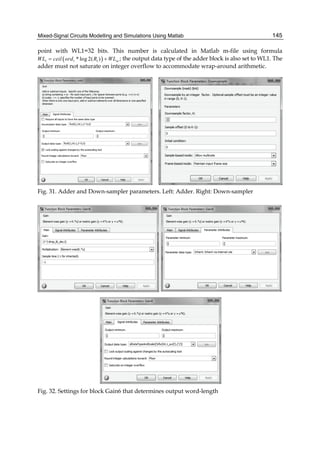
modelled in Simulink as a noise source by using a block “Random source” (see Fig. 20
for the 2nd integrator). The parameters are set as follows: “Source type” to Gaussian,
“Mean” to 0, “Variance” to noise power according to (14), “Sample mode” to discrete,
“Sample time” to Ts, “Samples per frame” to 1, “Output data type” to Double, and
“Complexity” to Real.
Fig. 20. kT/C noise modelling adding Random source to each S-C stage](https://image.slidesharecdn.com/engineeringeducationandresearchusingmatlab-160628213608/85/Engineering-education-and_research_using_matlab-145-320.jpg)
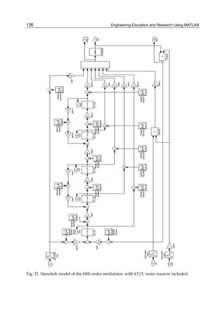


![Engineering Education and Research Using MATLAB142
Fig. 27. BS spectrum of the example modulator for nonlinear Quantizer model. Left spectrum:
Gcomp=1000, Right spectrum: Gcomp=100
Fig. 28. Spectrum of the BS of the fifth order modulator, with non-ideal effects included. Left
spectrum: No noise circuit included, Right spectrum: All noise sources and all other non-
ideal effects included
Fig. 28 shows two simulation results. Both are calculated from the bit-stream of our fifth
order example modulator. All non-ideal effects are included with parameters given in (23).
[ ]
[ ]
[ ]
0, 1000; 1...5
5 ; 1...5
70, 38,14, 8, 8
15, 40, 80, 80,80
150
i
i s
ndop
A i
BW f Hz i
V
s
nV
Hz
Temp C
μ
°
= =
= ⋅ =
⎡ ⎤
= ⎢ ⎥
⎣ ⎦
⎡ ⎤
= ⎢ ⎥
⎣ ⎦
=
SR
V
(23)](https://image.slidesharecdn.com/engineeringeducationandresearchusingmatlab-160628213608/85/Engineering-education-and_research_using_matlab-152-320.jpg)


![Control Optimization Using MATLAB 153
3. LQR regulator with feed-forward controller
The second problem requires a Control System Toolbox since it is an extended version of the
problem from the Simulink demo lqgdemos file.
The SISO application can be modelled as a linear ranking 4 system with an enlarging
saturation by ± 5 and a non-linear limit of error of ± 10.
The equations are (Franklin, G., et al., 1987; Potvin, A. F., 1991; National Instruments;
MathWorks; MathWorks User’s Guide, 2003):
[ ]
1.0285 0.9853 0.9413 0.0927 0
1.2983 1.0957 2.8689 4.7950 6.6389
0.1871 3.8184 2.0788 0.9781 0
0.4069 4.1636 2.5407 1.4236 0
1.7786 1.1390 0 1.0294
x x u Ax Bu
y Cx
− −⎡ ⎤ ⎡ ⎤
⎢ ⎥ ⎢ ⎥− −⎢ ⎥ ⎢ ⎥= + = +
⎢ ⎥ ⎢ ⎥− − −
⎢ ⎥ ⎢ ⎥
− −⎣ ⎦ ⎣ ⎦
= − − =
(3)
They define the nominal plant model. One allows the installation’s matrix to vary between
half to two times of its nominal value.
Using LQG / LTR techniques, one can design a Kalman state estimator and a k amplifier
regulator for the linear system. Add an integrator to ensure a zero steady error.
To achieve an increased time response one adds a feed-forward amplifier (FF).
In the demo Simulink Iqgopt system, the control parameters k and FF are granted by ‘the
method presented above (National Instruments; MathWorks; MathWorks User’s Guide, 2003).
These parameters can be accorded using the NCD Blockset.
In particular the control parameters k and FF are granted, so that the closed-cycle system
may meet the following specifications:
• Maximum oscillation - 20%;
• Propagation time - one second;
• Response time - three seconds (Franklin, G., et al., 1987; Potvin, A. F., 1991; National
Instruments; MathWorks; MathWorks User’s Guide, 2003).
The Simulink system contains the application and the control structure below:
After starting the system, it is noted that the non-linearity error (± 10) and the saturation (± 5)
are included in the model’s installation.
Using the From Workspace block, one introduces a step that goes from zero to one in one
second. An NCD block is attached to the result of the installation because there is a
restricted signal. Checking the System’s Parameters one observes that each simulation
always lasts 10 seconds.
Tunable and uncertain variables are initialized. Domain restrictions for this demonstration
are defined. Upper and lower restriction limits on the oscillation, propagation time and
response time are defined. As described above, an initial design regulator using the LQG /
LTR methods is designed starting from a linear application. For non-linear control
optimization the feed-forward amplifier FF and regulatory matrix amplifier k are tunable
(Franklin, G., et al., 1987; Potvin, A. F., 1991; National Instruments; MathWorks; MathWorks
User’s Guide, 2003).
Note how the installation (reaction) matrix A is defined and also that the optimization
restrictions are applied only on nominal installation (reaction).](https://image.slidesharecdn.com/engineeringeducationandresearchusingmatlab-160628213608/85/Engineering-education-and_research_using_matlab-163-320.jpg)


![Control Optimization Using MATLAB 161
The aim of the study is to stabilize the inverted pendulum so that the position of the carriage
on the track is controlled quickly and accurately so that the pendulum is always erected in
its inverted position during such movements.
The inverted pendulum (IP) is among the most difficult systems to control in the field of
control engineering. Due to its importance in the field of control engineering, it has been a
task of choice to be assigned to control engineering students to analyze its model and
propose a linear compensator according to the PID control law (Sultan, K., 2003, 2007).
For device, a stabilized runway requires the existence of the initial LQR stabilizer. The
generation of this regulator rules is realized starting with writing the non-linear equations
which define the inverted pendulum. Ignoring the dynamics of the engine, the non-linear
equations of motion, for the inverted pendulum system, are (Franklin, G., et al., 1987;
Potvin, A. F., 1991; National Instruments; MathWorks; MathWorks User’s Guide, 2003):
2
sin sin cos
sin
f
l g
my
M
m
θ θ θ θ
θ
+ −
=
+
(6)
2
2
cos sin sin cos
sin
f M m
g l
m m
M
l
m
θ θ θ θ θ
θ
θ
+
− + −
=
⎛ ⎞
+⎜ ⎟
⎝ ⎠
(7)
Where:
• f is the force applied to the cart by the engine in Newton (N);
• m is the position of the cart in meters;
• y is the vertical angle of the pendulum in radians;
• θ is the mass of the cart (0.45 kg);
• M is the pendulum mass (0.21 kg);
• l is the distance from the mass centre of the pendulum (half of its length of 0.61 m);
• g is gravitational acceleration (m/s).
It is necessary that those equations to be linear in the operating point y=0 and (=0 to obtain
the linear system:
( )
0 1 0 0 0
11
0 0 0
0 0 0 1 0
1
0 0 0
y gm
y M Mx f Ax bx
g M m
lMlM
θ
θ
⎡ ⎤ ⎡ ⎤
⎢ ⎥ ⎢ ⎥⎡ ⎤
⎢ ⎥ ⎢ ⎥−⎢ ⎥
⎢ ⎥ ⎢ ⎥⎢ ⎥= = = +⎢ ⎥ ⎢ ⎥⎢ ⎥
⎢ ⎥ ⎢ ⎥⎢ ⎥
⎢ ⎥+ ⎢ ⎥⎣ ⎦ −⎢ ⎥ ⎢ ⎥⎣ ⎦⎣ ⎦
(8)
Using MATLAB command:
Klqr = lqr(A.b,diag( [0.25 0 4 0],0.003)
one obtains the gained stability:
K1qr = (-28.86 -28.56 -145.00 14 -14.86)
Besides the obvious non-linearity of the system’s equations, the voltage limit applied to the
engine gives a restriction of the action saturation of 1 N (Franklin, G., et al., 1987; Potvin, A.
F., 1991; National Instruments; MathWorks; MathWorks User’s Guide, 2003).](https://image.slidesharecdn.com/engineeringeducationandresearchusingmatlab-160628213608/85/Engineering-education-and_research_using_matlab-171-320.jpg)


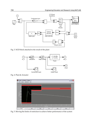
![Engineering Education and Research Using MATLAB164
To obtain a general model that can be used regardless of the values of mechanical
parameters of the system, the Simulink model will be developed with formal parameters.
But, before starting the simulation, the numerical values of mechanical parameters (m1, m2,
I2, b, g0) will be initialized in the MATLAB environment. The following scheme is done in
Simulink (Patic, P. C., Gorghiu, G., 2009; Stanciulescu, F., 2003):
Fig. 14. Simulink scheme regarding the arm modelling
The localization of the blocks in Simulink sub-libraries is (Patic, P. C., Gorghiu, G., 2009;
Stanciulescu, F., 2003):
x_A, x_B, x_C, 1/D, t_A, t_B, t_C, 1/D1 – blocks Fcn in Functions & Tables;
F, M – blocks Constant in Sources;
Sum, Sum1 – blocks Sum in Math;
Mux, Mux1 – blocks Mux in Signals&Systems;
Integrator, Integrator1, …. – blocks Integrator in Continuous;
Rad-grd – block Gain in Math;
FM, x1, Teta2 – blocks Scope in Sinks
The functions performed by each block are:
x_A: -(I2+m2*b^2*(sin(u[2]))^2)*m2*b*sin(u[2])*(u[1]^2);
x_B: -(m2*b)^2*sin(u[1])*cos(u[1])*g0;
x_C: (I2+m2*b^2*(sin(u[3]))^2)*u[1]-(m2*b*cos(u[3]))*u[2];
t_A: (m2*b)^2*sin(u[2])*cos(u[2])*(u[1]^2);
t_B: (m1+m2)*m2*b*sin(u[1])*g0;
t_C: -(m2*b*cos(u[3]))*u[1]+(m1+m2)*u[2];
1/D, 1/D1: u[1]/((m1+m2)*(I2+m2*b^2*(sin(u[2]))^2)-(m2*b*cos(u[2]))^2).](https://image.slidesharecdn.com/engineeringeducationandresearchusingmatlab-160628213608/85/Engineering-education-and_research_using_matlab-174-320.jpg)

![Engineering Education and Research Using MATLAB166
The block rad-grd being Gain type, with value 180/pi, transform the position θ2 from
radians to degrees, just for viewing. As a method of integration, we will choose the method
with variable step ode45, maximum integration step is imposed being 0.0001 [s], as well as
the final time (stop time), which is 10 [s]. The maximum step 0.0001 was chosen to track the
influence of changing values in the simulation stimuli on the evolution of the system
(Stanciulescu, F., 2003; Stareţu, I., Ionescu, M., 2005).
After the model realization, a MATLAB file by “m” type is created in which are initialized
the values of the mechanical parameters (Patic, P.C., Gorghiu, G., 2009):
m1=1;
m2=1;
I2=0.01;
b=0.2;
g0=9.81;
brat;
When typing in MATLAB window, the name of this file will be loaded in MATLAB space
with the mechanic’s parameter values, the last line of the file causing the opening model
(Stanciulescu, F., 2003).
The simulation will aim to highlight the evolution of the system to changes in external
stimuli.
The results exemplified correspond to a force application F = 2 [Nm] at time of t = 1 sec.
5.2.1 Simulation of the robotic arm using the 3rd degree polynomial interpolation
Continuing our study, for the proper representation of variations of positions, velocities and
accelerations for these study couplers robots, we used two methods, utilized very often, to
solve these problems of movements of a robot. The first method used was the 3rd degree
polynomial interpolation. The other method is the connection of linear functions in parables
(Pozna, C., 2000).
One can say that both methods transform the task space in joint coordinates. Polynomials
can be used to approximate more complicated curves. A relevant application is the
evaluation of the natural logarithm and trigonometric functions. This results in significantly
faster computations. Polynomial interpolation also forms the basis for algorithms in
numerical quadrate and numerical ordinary differential equations.
Polynomial interpolation is also essential to perform sub-quadratic multiplication and
squaring, where an interpolation through points on a polynomial which defines the product,
yields the product itself (Scritube Industrial Robots).
The interpolation polynomial of three degree is like below:
P(x) = a3x3 + a2x2 + a1x + a0 (9)
The statement that P interpolates the data points means that:
P(xi) = yi, where i∈{0, 1, 2, 3} (10)
The second method is the connecting of the linear functions in parables. This method is
generally used when the robot trajectory passes through several points, but can be used,
also, to move from point to point. To join two different points, rectilinear trajectories are
used and to respect the conditions of speed and acceleration (by crossing points) straight
paths are connected in parables.](https://image.slidesharecdn.com/engineeringeducationandresearchusingmatlab-160628213608/85/Engineering-education-and_research_using_matlab-176-320.jpg)


![Engineering Education and Research Using MATLAB178
4. Graphical MATLAB-based tool
A graphical user interface tool was designed using the Matlab GUIDE environment which
greatly simplifies the process of building and developing GUIs. GUIDE Layout Editor
allows the user to populate a GUI by clicking and dragging GUI components namely, axes,
panels, buttons, text fields, sliders into the layout area. Moreover, from the Layout Editor,
the user can size the GUI, modify component look and feel, align components, set tab order,
view a hierarchical list of the component objects, and set GUI options.
GUIDE automatically generates a program file containing MATLAB functions that controls
how the GUI operates. This code file helps initialize the GUI and contains a framework for
the GUI callbacks; the routines that execute when a user interacts with a GUI component.
The MATLAB Editor should be used to add code to callbacks in order to perform the
required actions [MATLAB Creating Graphical User Interfaces, 2004].
4.1 GUI layout and programming
The main window (Electronics Teaching Assistant) is designed to allow the user choose
between Operational Amplifier circuits and Electric Circuits and exit the tool as shown in
Fig. 9. It consists of two Axes, text and three push buttons namely, OP AMP Circuits,
Electric Circuits and Close. The two axes are used for presenting images: one for logo and
the other for background. The text displays the tool’s name. OP AMP Circuits button will
allow the user to analyze different types of OP AMP Circuits. Electric Circuits button will let
the user analyze different types of electric circuits (voltage and current dividers). Close
button will simply close the whole program.
The following code blocks show how the three buttons are programmed. The set function
set(handle, 'PropertyName', value) is used to set a property value of buttons.
% --- Programming theOP_AMP_Circuits_Button.
functionOP_AMP_Circuits_Button_Callback(hObject, eventdata, handles)
% hObject=handle to OP_AMP_Circuits_Button (see GCBO)
% eventdata= reserved to be defined in a future version of MATLAB
% handles = structure with handles and user data (see GUIDATA)
%---- To open Electric Circuits window ---------%
set(ETA_OP_AMP_Circuits,'Visible','on')
%---- To Close Electronics_Teaching_Assistant window ------%
set(Electronics_Teaching_Assistant,'Visible','off')
functionElectronic_Circuit_Button_Callback(hObject, eventdata, handles)
%---- To open Electric Circuits window ---------%
set(ETA_Electric_Circuits,'Visible','on')
%---- To close main window window ------------%
set(Electronics_Teaching_Assistant,'Visible','off')
functionClose_Button_Callback(hObject, eventdata, handles)
%---- To terminate the program ---------%
delete(get(0,'Children'));
In order to show the logo and background images and their axes, the code is written under
Opening Function. Axes function is used to determine which axes the image should
display followed by imshowfunction.](https://image.slidesharecdn.com/engineeringeducationandresearchusingmatlab-160628213608/85/Engineering-education-and_research_using_matlab-188-320.jpg)


![Engineering Education and Research Using MATLAB182
% 5 : Summing Amplifier
% 6 : Differential Amplifier
%------------------------------------------------------------------------%
switch get(handles.Circuit_Type_Popupmenu,'Value')
%---------------------------- Summing Amplifier---------------------------%
case 4
Vin2 = str2double(get(handles.Vin_2_Edit, 'string')) % Input voltage 2
Rf = str2double(get(handles.R_FEdit, 'string')); % input Resistor 3
%--------------Summing Equation -------------%
Gain_Result = -Rf/R1 % Gain 1
Gain_Result_2 = -Rf/R2 % Gain 2
%-------output voltage---------%
Vout_1 = Gain_Result * Vin
Vout_2 = Gain_Result_2 * Vin2
Vout = Vout_1+ Vout_2;
set(handles.Vout_Out_Text,'String',num2str(Vout))
n = 1; % one cycle
t = 0 :pi/8 : 2*n*pi % time domain
Vin_Plot = Vin * sin(t)
Vout_Plot = Vout * sin(t)
if (abs (Vout) <= abs(Power_Supply)) % Check if clipping problem is occurred
plot(t, Vin_Plot,'RED' ,'linewidth',2)
grid on
axis([ 0 max(t) -20 20])
hold on
plot(t, Vout_Plot,'GREEN' ,'linewidth',2)
grid on
xlabel('Time (t)','fontweight','bold')
ylabel('Input - Output Voltage (V)','fontweight','bold')
legend('Vin', 'Vout');
else
axes(handles.Vin_Vout_Axes)
Vin_Plot = Vin * sin(t)
Vout_Plot = Vout * sin(t)
for i = 1 : length(Vout_Plot)
if (Vout_Plot(i)>Power_Supply)
Vout_Plot(i)= Power_Supply
elseif (Vout_Plot(i) < -Power_Supply)
Vout_Plot(i)= -Power_Supply
end
end
plot(t, Vin_Plot,'RED' ,'linewidth',2)
grid on
axis([ 0 max(t) -20 20])
hold on
plot(t, Vout_Plot,'GREEN' ,'linewidth',2)
grid on](https://image.slidesharecdn.com/engineeringeducationandresearchusingmatlab-160628213608/85/Engineering-education-and_research_using_matlab-192-320.jpg)


![Engineering Education and Research Using MATLAB198
N= 365; NY= 10;
% N= 365 days of the year and NY= # years of model data used (1995-2004)
for k=1:N, % Day index of year
GSR(k)= mean( GSR_10yr (k:N:(NY-1)*N+k));
end
where GSR_10yr is the data sheet containing the daily mean GSR data array of size 3650
days (1995-2004). Similarly, we generate the 10-year average daily SSH from the sunshine
hours data.
2.1.1.2 Extra-terrestrial radiation parameters
Mean daily values of GSR data are calculated from the knowledge of the latitude and
longitude in the city of Al-Ain (Latitude = 240 16’ and Longitude = 550 36’). The
extraterrestrial solar radiation on horizontal surface in kWh/m2 (G0) and theoretical
maximum daily sun hours (S0) are calculated from the equations (Assi et al., 2010):
[ ]0
24G 360
G 1 0.033cos cos( )cos( )sin( ) sin( )sin( )
365
SC
s s
n
π
⎡ ⎤⎛ ⎞
= + φ δ ω + ω φ δ⎜ ⎟⎢ ⎥
⎝ ⎠⎣ ⎦
(1)
0
2
15
sS = ω (2)
where n is the day index, ωs the mean sunrise hour angle for the month, φ the latitude, and δ
the declination angle. GSC is a constant representing the daily extraterrestrial solar radiation
on horizontal and is given by 1.367 kWh/m2. The declination angle (δ) is defined by the
equation:
[ ]1 2 n 28423.45
sin sin sin
180 365
−
⎡ ⎤⎛ ⎞π +π⎛ ⎞
δ = ⎢ ⎥⎜ ⎟⎜ ⎟
⎝ ⎠⎢ ⎥⎝ ⎠⎣ ⎦
(3)
The GSR and SSH data are next normalized to the extraterrestrial values G0 and S0 described
in eq. (1)-(2), and the resulting normalized data arrays denoted by clearness index
(RSSH=GSR/G0) and Sunshine duration ratio (RSSH = SSH/S0) are stored in excel file
solardata.xlsx in the form:
>> gsrdata=[N, S0, G0, RSSH, RGSR];
>> s=xlswrite('solardata.xlsx',gsrdata,'Sheet1', 'A1:E365');
The RGSR-RSSH data is then fitted to different nonlinear regression models as per Table 1.
Model reference Type Equation
(Podesta, 2004) Linear y= b1+b2* x
(Akinoglu & Ecevit, 1990) Quadratic y= b1+b2* x+b3* x2
(Samuel, 1991) Cubic y= b1+b2* x+b3* x2+b4* x3
(Ampratwum & Dorvlo, 1999) Logarithmic y= b1+ b2 *log( x)
(Newland, 1988) Log-Linear y= b1+ b2* x+ b3*log( x)
(Elagib & Monsell, 2000) Exponential y= b1* exp(b2*x)
Table 1. Nonlinear empirical regression models used for Al-Ain, UAE weather data](https://image.slidesharecdn.com/engineeringeducationandresearchusingmatlab-160628213608/85/Engineering-education-and_research_using_matlab-208-320.jpg)
![MATLAB-Assisted Regression Modeling of Mean Daily Global Solar Radiation in Al-Ain, UAE 199
2.1.1.3 MATLAB application in nonlinear regression
The nonlinear regression in MATLAB is performed using two tools:
1. Interactive nonlinear regression toolbox (nlintool )
2. Nonlinear mixed-effects estimation (nlmefit)
The procedure followed in each approach is discussed in the next sections including sample
output results from the weather GSR modeling. Alternative approaches include specifically
written MATLAB m-files or the use of commercial statistical software packages such as
SPSS, Minitab or SAS. All our MATLAB results agree well with results obtained using SPSS
and Minitab.
2.1.1.3.1 Use of the interactive nonlinear regression toolbox (nlintool)
The MATLAB procedure to use “nlintool” is explained through the application of the log-
linear regression model, described in Table 1, to model the relation between the clearness
index (RGSR) and sunshine duration ratio (RSSH) through the following steps:
1. Given RSSH and RGSR data (N points each). Read the input data to MATLAB
workspace from an Excel data sheet “GSRdata.xlsx” as follows:
>> inputdata=xlsread (‘GSRdata.xlsx’, ‘sheet1’,’A1:B365’)
>> RSSH=inputdata(:,1);
>> RGSR=inputdata(:,2);
The input data array contains two columns of length N=365, namely, RSSH
(independent variable or predictor) and RGSR (dependent variable).
2. Next, generate an m-file script called “loglinear.m” containing the regression function
as follows:
function yhat = loglinear(beta, x)
b1 = beta(1);
b2 = beta(2);
b3 = beta(3);
yhat = b1 + b2*x + b3*log(x);
3. In command window type:
>> beta0=[ 0 0 0]; % define initial guess of constants beta(k), k=1,2,3
>> nlintool(RSSH, RGSR,@loglinear,beta0) % Invoke the interactive
nonlinear regression toolbox
The output is the log-linear regression curve with error bounds as shown in Fig. 1.
4. Data that can be downloaded to MATLAB workspace include the regression
coefficients (beta) and root-mean square error (rmse). This is done as follows:
>> rmse % root mean-square error
rmse =
0.0262
>> beta % regression model coefficients
beta=
-0.1778 6.1287E-05 0.2251](https://image.slidesharecdn.com/engineeringeducationandresearchusingmatlab-160628213608/85/Engineering-education-and_research_using_matlab-209-320.jpg)
![Engineering Education and Research Using MATLAB200
Fig. 1. Nonlinear regression curve with a log-linear function between Clearness index (RGSR)
and sunshine duration ration (RSSH)
The command “whos” provides information on available workspace variables. Similarly,
other nonlinear regression curve fits could be obtained by generating the corresponding m-
file for each regression function and specifying the corresponding initial guess values for the
unknown parameters.
Table 2 shows the coefficients obtained for each regression model shown in Table 1. The
statistical error parameters resulting from each regression model can be computed using
SPSS, Minitab or using MATLAB from the expressions displayed in section 2.3.
Type Equation b1 b2 b3 b4
Linear y= b1+b2* x 0.4619 0.0047
Quadratic y= b1+b2* x+b3* x2 0.2980 0.0118 -7.400E-05
Cubic y= b1+b2* x+b3* x2+b4* x3 8.4297 -0.5183 0.0114 -8.2410E-05
Logarithmic y= b1+b2*log( x) -0.1697 0.2223
Log-Linear y= b1+ b2* x+ b3*log( x) -0.1778 -6.133E-05 0.2252
Exponential y= b1* exp(b2*x) 0.4948 0.0069
Table 2. Estimated coefficients for empirical regression models of weather data for years
1995-2004 in Al-Ain, UAE. Variables are y = RGSR = GSR/G0 and x = RSSH = SSH/S0
2.1.1.3.2 Use of the nonlinear mixed-effects estimation (nlmefit)
The nonlinear regression in MATLAB can also be performed using the nonlinear mixed-
effects estimation (nlmefit). This tool fits the model by maximizing an approximation to the
marginal likelihood with random effects integrated out, assuming that [See MATLAB help]
random effects are multivariate normally distributed and independent between groups, and
that observation errors are independent, identically normally distributed, and independent
of the random effects. As an example, the format for the log-linear regression equation is as
follows:](https://image.slidesharecdn.com/engineeringeducationandresearchusingmatlab-160628213608/85/Engineering-education-and_research_using_matlab-210-320.jpg)
![MATLAB-Assisted Regression Modeling of Mean Daily Global Solar Radiation in Al-Ain, UAE 201
>> model = @(phi,t)(phi(:,1)+ phi(:,2).*t + phi(:,3).*log(t));
>> phi0 =[0 0 0];
>> group=[1:365];
>> [beta,psi,stats] = nlmefit(RSSH(:),RGSR(:),group,[],model,phi0)
The arguments of the MATLAB function ‘nlmefit’ used for our regression are:
RSSH: is an n-by-1 array of n observations on 1 predictor.
RGSR: is an n-by-1 vector of responses.
Group: is a grouping variable indicating m groups in the observations. Here, we enter size
of rows of predictors, i.e. group=[1:365].
Model: is a function handle that accepts predictor values and model parameters and
returns fitted values.
phi0: contains the initial values of the regression for equation parameters.
The program outputs are:
beta= contains the estimated regression model parameters
psi= an r-by-r estimated covariance matrix for the random effects. By default, r is equal
to the number of model parameters p.
stats= returns a structure with the following parameters:
• logl — The maximized log-likelihood for the fitted model
• mse — The estimated error variance for the fitted model
• aic — The Akaike information criterion for the fitted model
• bic — The Bayesian information criterion for the fitted model
• sebeta — The standard errors for beta
• dfe — The error degrees of freedom for the model
The following is the MATLAB output to the log-linear regression model:
beta =
-0.1778
-6.1336E-05
0.2252
psi =
1.0e-003 *
0.6821 0 0
0 0.0000 0
0 0 0.0000
stats =
logl: 8.1257e+002
mse: 3.7845e-028
rmse:1.9454e-014
aic: -1.6111e+003
bic: -1.5838e+003
sebeta: [1.3834 0.0104 0.4869]
dfe: 358
The regression model parameters obtained using the ‘nlmefit’ function match with the
values computed using the “nlintool” function and listed in Table 2. The best regression](https://image.slidesharecdn.com/engineeringeducationandresearchusingmatlab-160628213608/85/Engineering-education-and_research_using_matlab-211-320.jpg)

![MATLAB-Assisted Regression Modeling of Mean Daily Global Solar Radiation in Al-Ain, UAE 203
2.1.2 Time-series regression modelling with ARIMA approach
The time-series regression modelling approach makes use of the four weather parameters
measured daily over a period of 10 years, i.e. 1995-2004 in Al-Ain, UAE. These parameters
are:
1. Mean daily temperature (0C) abbreviated as T
2. Mean daily wind speed (knots) abbreviated as W
3. Daily sunshine hours abbreviated as SSH
4. Mean daily relative humidity (%) abbreviated as RH
5. Mean daily global solar radiation (kWh/m2) abbreviated as GSR
The modeling procedure steps are as follows:
Step 1. Explore the form and characteristics of the dependent variable (GSR) and the
predictors (T, W, SSH and RH) by looking at their time-series plots with the help of
MATLAB. These plots will help in identifying the behavior of each variable and to
check the trend and seasonality of GSR data.
Step 2. Compute the descriptive statistics of the four independent variables (T, W, SSH,
and RH) and the dependent variable (mean daily GSR). The correlation between
these variables is shown in Table 3. It shows that wind speed has the least effect on
GSR performance. From the time-series plots of GSR, T and SSH data we can
observe a cyclical behavior. Wind and humidity data on the other hand are more
random. The best model is obtained when all four independent variables are
considered in the GSR regression model.
T W SSH RH GSR
T 1.0000 0.1907 0.4555 -0.7419 0.7958
W 0.1907 1.0000 -0.1099 -0.2170 0.1425
SSH 0.4555 -0.1099 1.0000 -0.4566 0.6972
RH -0.7419 -0.2170 -0.4566 1.0000 -0.6761
GSR-kWh/m2 0.7958 0.1425 0.6972 -0.6761 1.0000
Table 3. Correlation between the measured weather data parameters for the city of Al-Ain,
UAE for years 1995-2004
The Pearson correlation values between the response (GSR) and the four predictor variables
(T, W, SSH, RH) are found in MATLAB using the command:
>> corr(T, W, SSH, RH, GSR)
Table 3 shows that the temperature and sunshine hours have dominant effect on the GSR
parameter followed closely by relative humidity and with less influence by wind speed.
The computation of the descriptive statistics can be done directly in SPSS or Minitab. In
MATLAB we can either write a script m-file to compute all needed statistical parameters or
we can use the already available functions in MATLAB and other functions that can be run
under the Statistics toolbox. One MATLAB command that generates some statistical
parameters is:
>> [xds,yds] = datastats (xdata, ydata)](https://image.slidesharecdn.com/engineeringeducationandresearchusingmatlab-160628213608/85/Engineering-education-and_research_using_matlab-213-320.jpg)
![Engineering Education and Research Using MATLAB204
which returns statistics for the column vectors xdata and ydata to the structures xdata and
ydata, respectively. xdata and ydata must be of the same size. The returned statistics
include: sample size, maximum value, minimum value, mean, median, range, and standard
deviation. MATLAB also has standalone functions for statistical values such as: max, min,
length (sample size), mean, median, mode, std (standard deviation), and var (variance). The
coefficient of variation is found from the ratio of std(x)/mean(x). One can also use hist(x) to
get a histogram of the sample data. Other statistical measures need to be programmed or
can be determined using the MATLAB Statistics toolbox. Table 4 lists the commands that
can be employed to obtain the central and dispersion measures for the data sets under study.
Central Measures Dispersion Measures
Command Description Command Description
geomean Geometric mean iqr Interquartile range
harmean
Harmonic Mean absolute
deviation
mad Mean absolute deviation
mean Arithmetic mean moment
Central moment of all
orders
median 50 % Percentile range Range
trimmean Trimmed mean std Standard deviation
mode Most frequent value var Variance
Table 4. MATLAB commands for computing central and dispersion measures of a data set
The following commands can be used under the Statistics toolbox:
>> locate = [geomean(x) harmmean(x) mean(x) median(x), trimmean(x,25)]
>> stats = [iqr(x) mad(x) range(x) std(x)]
On the other hand, measures of shape are found using quantiles (0 < p < 1) or percentiles
(0< p <100). The percentiles for a data sequence xdata are found in the Statistics toolbox
using the command:
>> y = prctile(xdata,p); % p= percentile needed
>> y = quantile(xdata,p); % p= quantileneeded
The shape of a data distribution is also measured by the Statistics Toolbox functions
skewness, kurtosis, and, more generally, moment.
Table 5 shows the descriptive statistics obtained for the mean daily global solar radiation
data for Al-Ain, UAE for period 1994-2005.
Step 3. Fig. 4 shows the time-series plot of the mean daily GSR for years 1995-2004 with
leap days excluded. The plot shows a clear periodicity of one year (365 days).
Step 4. The partial least square regression technique is used to model the relation between
GSR data for ten years (1995-2004) and the four aforementioned dependent weather
variables. The model equation obtained using MATLAB or using either software
packages SPSS or Minitab is of the form:
regression 1 2 3 4 5GSR (t) a a T(t) a W(t) a (t) a RH(t)SSH= + ∗ + ∗ + ∗ + ∗ (4)
where the regression coefficients are given in Table 6.](https://image.slidesharecdn.com/engineeringeducationandresearchusingmatlab-160628213608/85/Engineering-education-and_research_using_matlab-214-320.jpg)
![MATLAB-Assisted Regression Modeling of Mean Daily Global Solar Radiation in Al-Ain, UAE 205
Statistical Parameters T W SSH RH GSR
Mean ( μ ) 36.501 7.5305 9.9472 44.0450 6.3332
StdDev ( σ ) 7.7250 1.9896 1.5849 16.8160 1.3962
SE Mean( / Nσ ) 0.1280 0.0329 0.2620 0.2780 0.0231
Variance ( 2
σ ) 59.6690 3.9585 2.5121 282.7660 1.9494
CoefVar ( σ/μ ) in % 21.1600 26.4200 15.9300 38.1800 22.0500
Min 16.2000 0.2084 0.8000 7.3750 1.1350
Median 37.6000 7.2506 10.2000 43.4170 6.5540
Max 49.1000 22.7936 12.8000 97.2300 8.8210
Skewness (σk) -0.3000 1.6000 -1.5200 0.2000 -0.3600
Kurtosis (ku) -1.2100 5.7300 3.7700 -0.7000 -0.9000
Table 5. Descriptive data statistics for the measured weather data parameters for the city of
Al-Ain (Years 1995-2004) where N= 3650 data samples
Fig. 4. Daily mean Global Solar Radiation (GSR) in Al-Ain, UAE for years 1995-2004
Coefficient a1 a2 a3 a4 a5
Value -1.1973 0.0971 0.0513 0.3850 - 0.0052
Table 6. Regression coefficients of eq. (4)
The regression model of eq. (4) yields a deterministic coefficient R2 = 0.7824 and
MSE = 0.4247. In MATLAB, the regression between GSR and predictor variables (T, W, SSH,
RH) is done using the Statistics Toolbox command
>> regcoef= robustfit(xdata, GSR )
Where ‘xdata‘ is an array matrix containing the four predictors, i.e. xdata=[T, WS, SSH, RH],
and ‘regcoef‘ is a vector returning the regression coefficients between GSR and the four
predictor weather variables resulting from the robust multi-linear regression process. The
correlation between the regression component GSRregression and GSR can be found using
>> corr(GSR, GSRregression)](https://image.slidesharecdn.com/engineeringeducationandresearchusingmatlab-160628213608/85/Engineering-education-and_research_using_matlab-215-320.jpg)
![Engineering Education and Research Using MATLAB206
Step 5. Trend and Seasonality components of the residual regression error
The residual error from the multivariate linear regression model in eq. (4), denoted by
GSRresidue1 (t) = GSR - GSRregression(t), is shown in Fig. 5. The objective is to first examine it for
trends and/or seasonality and decompose it to yield:
residue1 trend seasonal residue2GSR (t) GSR (t) GSR (t) GSR (t)= + + (5)
Fig. 5. Residual term of mean daily GSR after subtracting regression model of eq. (4)
The trend component is extracted in MATLAB using the statement
>> gsrdet=detrend(gsrresidue1`); % This gives GSRresidue1 with trend removed
>> gsrtrend=gsr-gsrdet;
The trend equation can be deduced using the cftool command in MATLAB that invokes the
curve fitting GUI and then performs a linear polynomial fit to yield the linear trend
equation:
trendGSR (t) 0.0771 4.2211E 05 t= − − ∗ (6)
The mathematical model for the seasonal component, i.e. GSRseasonal(t), is found from
MATLAB using the FFT algorithm. The resulting model is:
NP 1
2
seasonal k k1
2 2
GSR (t) a cos kt b sin kt
NP NPk
−
=
⎡ ⎤π π⎛ ⎞ ⎛ ⎞
= +⎜ ⎟ ⎜ ⎟⎢ ⎥
⎝ ⎠ ⎝ ⎠⎣ ⎦
∑ (7)
The MATLAB statement to generate the Fourier Coefficients for a periodic sequence
(period=NP=365) of data x[n], n=1, 2,.., N=3650 is done using:
>> N=3650;
>> y=fft(x,N); % here x is an array representing the de-trendedGSR residual](https://image.slidesharecdn.com/engineeringeducationandresearchusingmatlab-160628213608/85/Engineering-education-and_research_using_matlab-216-320.jpg)


![MATLAB-Assisted Regression Modeling of Mean Daily Global Solar Radiation in Al-Ain, UAE 209
to yield a parsimonious ARMA model, whilst passing the diagnostic checks. A parsimonious
model is desirable because including irrelevant lags in the model increases the coefficient
standard errors and therefore reduces the t-statistics. Models that incorporate large numbers
of lags tend not to forecast well as they fit data specific features, explaining much of the
noise or random features in the data. Therefore, model coefficients with p-values higher
than 0.05 are insignificant and should be eliminated to avoid over-fitting as they have little
effect on the prediction model (Enders, 2010). Different models can be obtained for various
combinations of AR and MA individually and collectively. The best model is selected using
the following diagnostics:
(a) Low Akaike Information Criteria (AIC)/ Schwarz-Bayesian Information Criteria (SBC,
BIC)
These model parameters are dependent on the data sample size, model mean-square error
(MSE), and the (p, q) values of the ARMA model. Their definition can be found in MATLAB
help (MATLAB, 2010) or (Enders, 2010). SBC selects the more parsimonious model and is
better than AIC for large samples. The best model should have the lowest AIC/SBC value and the
least MSE.
(b) Plot of residual autocorrelation function (ACF)
The appropriate ARMA model, once fitted, should have a residual error whose ACF plot
varies within the 95% CI bounds ( 1.96 / N± ) where N is the number of observations upon
which the model is based.
(c) Non-significance of auto correlations of residuals via Portmanteau tests (Q-tests based
on Chi-square statistics) such as Box-Pierce or Ljung-Box tests(White noise tests)
Once the optimal ARMA(p,q) model for the residual GSR time-series is selected, there is a
need to check the white noise test if the ACF/PACF correlograms show significant spikes at
one or more lags that could be just by chance. These tests indicate whether there is any
correlation in the time-series or whether the abnormal spikes encountered in the ACF and
PACF of the residual error are just a set of random, identically distributed variables overall.
The Ljung-Box Q-statistics can be used to check if the residuals from the ARMA(p, q) model
behave as a white-noise process (Ljung & Box, 1978; Enders, 2010). Ljung & Box use the Q
statistic:
( )( )
2
1
2
K k
k
r
Q n n
n k=
= +
−
∑ (10)
which yields a more accurate variance of ACF [variance becomes (n-K)/n2 instead of 1/n]
compared to the statistic defined earlier by(Box & Pierce, 1970). K is the degrees of freedom
representing the maximum lags considered (normally 20). n = N-d with N being the number
of data points and d the degree of differencing (no differencing is assumed in this work so d
= 0), and rk is the sample ACF at lag k.
Under the null-hypothesis that all values of autocorrelation rk = 0, the Q Statistic is
compared to critical values from chi-square distribution χ2 distributed with K-degrees of
freedom. If the model is correctly specified, the residuals should be uncorrelated and Q
should be small and consequently the probability value should be large. A white noise
process would ideally have Q = 0. Therefore, if Q > 2
,DF αχ at the specified DF and
significance level α, then the we can reject the null hypothesis.](https://image.slidesharecdn.com/engineeringeducationandresearchusingmatlab-160628213608/85/Engineering-education-and_research_using_matlab-219-320.jpg)

![MATLAB-Assisted Regression Modeling of Mean Daily Global Solar Radiation in Al-Ain, UAE 211
Fig. 8. ACF and PACF plots for the residual error of the ARMA(2, 1) model
The MATLAB function “roots(c)” computes the roots of the polynomial P(x) whose
coefficients are the elements of the vector c. If c has (n+1) components, the polynomial is
P(x)=c(1)*xn+ ... + c(n)*x + c(n+1).
Next, the ARMA(2,1) model parameters φ(B) obtained from SPSS are used in MATLAB to
perform the stationarity unit-root test as follows :
>> phi=[1.4504 -0.4568];
>> phiB=[-phi(end:-1:1), 1]
phiB=
0.4568 -1.4504 1
>> roots(phiB) % find roots of polynomial with coefficients phiB
ans =
2.1631
1.0120
Note that all roots of φ(B) lie outside the unit circle thus implying a stationary ARMA(2, 1)
model. Once the ARMA(p, q) model is selected and checked for stationary residual error,
the GSR regression model involving the ARMA model becomes:
regression trend seasonal ARIMAGSR(t) GSR (t)+ GSR (t) GSR (t) GSR (t)+ WN(t)= + + (14)
where WN(t) is the final residual error which resembles white noise with zero mean and
constant variance.](https://image.slidesharecdn.com/engineeringeducationandresearchusingmatlab-160628213608/85/Engineering-education-and_research_using_matlab-221-320.jpg)


![Engineering Education and Research Using MATLAB214
3210-1-2-3
99.99
99
95
80
50
20
5
1
0.01
Residual Error
Percent
Mean 0.00005848
StDev 0.3364
N 3650
KS 0.074
P-Value <0.010
Normality Test for Residual Error
Normal
Fig. 11. Normality test for residual error with Minitab
Parameter
Regression vs.
Measured
Regression with ARMA
vs. Measured
95% CI on ratio of variances ] 0.976, 1.111 [ ] 0.979, 1.115 [
Ratio of variances 1.041 1.045
F (Observed value) 1.041 1.045
F (Critical value) 1.067 1.067
DF1, DF2 3649, 3649 3649, 3649
p-value (Two-tailed) 0.2204 0.1823
Table 10. Fisher's two-tailed F-test for the model data of 10 years
Levene’s equal variances test can also be applied as shown in Table 11. As the computed p-
value in Tables 11 is greater than the significance level alpha=0.05, one cannot reject the null
hypothesis H0. The risk to reject the null hypothesis H0 in Levene’s test while it is true is
55.62% and 43.96% for Regression and Regression with ARMA cases, respectively. Levene’s
test is mostly used in samples with normal distribution.
Parameter
Regression Vs
Measured
Regression with ARMA Vs
Measured
F (Observed value) 0.346 0.597
F (Critical value) 3.843 3.843
DF1, DF2 1, 7298 1, 7298
p-value (one-tailed) 0.5562 0.4396
Table 11. Levene's two-tailed variance test
2.1.2.5 Validation of time-series regression model
In the following section, the time-series regression model is validated with measured test
data set for years 2005-2007 in Al-Ain, UAE. A MATLAB code is written to implement the
regression model for the input test data (1095 points). The generated regression model test](https://image.slidesharecdn.com/engineeringeducationandresearchusingmatlab-160628213608/85/Engineering-education-and_research_using_matlab-224-320.jpg)


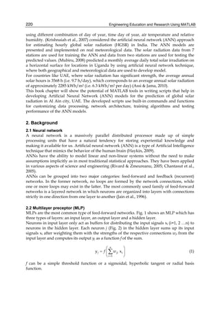


![Using MATLAB to Develop Artificial Neural Network Models for
Predicting Global Solar Radiation in Al Ain city – UAE 229
Fig. 7. Flow Chart for developing MLP and RBF networks using MATLAB
Training_Set = Shuffling_Inputs(1:3650,1:4)% specify training set [1995 - 2004]
Target_Set = Shuffling_Inputs(1:3650,5) % specify target set [1995 - 2004]
Testing_Set = Testing_Data(1:1095,1:4) % specify Testing set [2005- 2007]
Testing_Target_Set = Testing_Data(1:1095, 5) % specify Testing set, Target [2005- 2007]](https://image.slidesharecdn.com/engineeringeducationandresearchusingmatlab-160628213608/85/Engineering-education-and_research_using_matlab-239-320.jpg)
![Engineering Education and Research Using MATLAB230
A normalization process is applied for training and testing the data. Function “mapstd” is
used to normalize the inputs and target in order to yield zero mean and unity standard
deviation. The output is converted back into the same unit that is used for the original
target. Training and testing data are converted to rows (MATLAB requires that all data must
be presented as row vectors).
[pn, ps] = mapstd(Training_Set');
[tn, ts] = mapstd(Target_Set');
The settings structures pn and tn contain normalized values of inputs and output,
respectively, while ps and ts contain the means and standard deviations of the original
inputs and targets.
MATLAB helps devise the MLP model by using the built-in function “newff” which creates
a feed-forward back-propagation network. The designer can specify the number of hidden
layers, the neurons in each layer, the transfer function in each layer, the training function,
the weight/bias learning function, and the performance function. Moreover, this command
will automatically initialize the weights and biases. The function is called as follows:
MyNetwork = newff(pn,tn, [i] , {tf});
where the arguments pn and tn are the normalized input and output, respectively. [i]
implies that the network structure consists of one hidden layer and “i” neurons. For “j”
hidden layers we use [i, j]. The argument {tf} denotes the transfer function of the ith layer.
The network is next configured as follows
MyNetwork.trainFcn = LM;
MyNetwork.trainparam.min_grad = 0.00000001;
MyNetwork.trainParam.epochs = 1000;
MyNetwork.trainParam.lr = 0.4;
MyNetwork.trainParam.max_fail =20;
where
“trainFcn”: defines the function used to train the network. It can be set to the name of any
training function (LM ='trainlm'; %Levenberg-Marquardt back-propagation)
“trainparam.min_grad”: denotes the minimum performance gradient
“trainParam.epochs”: denotes the maximum number of epochs to train
“trainParam.lr”: denotes the learning rate
“trainParam.max_fail”: denotes the maximum validation failures
The function “newrb” is used for iteratively creating an RBF network by including one
neuron at a time. Neurons are added to the network until the sum squared error is found to
be very small or the maximum numbers of neurons are reached. The call for this function is:
MyNetwork= newrb(pn,tn,goal,spread, mn, df);
where pn and tn are the input and target, respectively. The argument “goal” denotes the
mean squared error goal, set here to be 0.01, and “spread” represents the spread of radial
basis functions, changed between 1 and 60 and denoted here as “i”. The argument “mn” is
the maximum number of neurons, changed between 5 and 600 and denoted here “j’, while
“df” represents the number of neurons to add between displays and is set to 50.
The MLP network is trained using the “trainFcn” and “trainParam” train functions. The
trained network is then saved in MATLAB by calling the functions
MyNetwork = train(MyNetwork,pn,tn);
save(NetworkName,'MyNetwork');
“NetworkName“ is a variable name which can be changed according to the network train
function and configuration in order to yield a meaningful name.](https://image.slidesharecdn.com/engineeringeducationandresearchusingmatlab-160628213608/85/Engineering-education-and_research_using_matlab-240-320.jpg)


![2 Will-be-set-by-IN-TECH
2. Fractional calculus fundamentals
2.1 Special functions
Here we should mention the most important function used in fractional calculus - Euler’s
gamma function, which is defined as
Γ(n) =
∞
0
tn−1
e−t
dt. (1)
This function is a generalization of the factorial in the following form:
Γ(n) = (n − 1)! (2)
This gamma function is directly implemented in the Matlab with syntax []=gamma().
Another function, which plays a very important role in the fractional calculus, was in fact
introduced in 1953. It is a two-parameter function of the Mittag-Leffler type defined as
(Podlubny, 1999):
Eα,β(z) =
∞
∑
k=0
zk
Γ(αk + β)
, (α > 0, β > 0). (3)
The Mittag-Leffler function (3) can be expressed in the integral representation as
Eα,β(z) =
1
2πi C
tα−βet
tα − z
dt, (4)
the contour C starts and ends at −∞ and circles around the singularities and branch points of
the integrand.
There are some relationships (given e.g. in (Djrbashian, 1993; Podlubny, 1999)):
E1,1(z) = ez
, E1/2,1(
√
z) =
2
√
π
e−z
erfc(−
√
z),
E2,1(z) = cosh(
√
z), E2,1(−z2
) = cos(z), E1,2(z) =
ez − 1
z
.
For β = 1 we obtain the Mittag-Leffler function in one parameter (Podlubny, 1999):
Eα,1(z) =
∞
∑
k=0
zk
Γ(αk + 1)
≡ Eα(z). (5)
For the numerical evaluation of the Mittag-Leffler function (3) with the default accuracy set
to 10−6 the Matlab routine [e]=mlf(alf,bet,c,fi), written by Podlubny and Kacenak
(2005) can be used. Another Matlab function f=gml_fun(a,b,c,x,eps0) for a generalized
Mittag-Leffler function was created by YangQuan Chen (Chen, 2008).
In Fig. 1(a) and Fig. 1(b) are plotted the well-known functions (ez and cos(z)) computed via
the Matlab routine []=mlf() created for the evaluation of the Mittag-Leffler function.
Another important function Ek(t, λ; μ, ν) of the Mittag-Leffler type was introduced by
(Podlubny, 1999). The function is defined by
Ek(t, λ; μ, ν) = tμk+ν−1
E
(k)
μ,ν(λtμ
), (k = 0, 1, 2, . . .), (6)
240 Engineering Education and Research Using MATLAB](https://image.slidesharecdn.com/engineeringeducationandresearchusingmatlab-160628213608/85/Engineering-education-and_research_using_matlab-250-320.jpg)
![Fractional Derivatives, Fractional Integrals, and Fractional Differential Equations in Matlab 3
−2 −1 0 1 2
0
2
4
6
8
z
E1,1
(z)
(a) E1,1(z), where −2 < z < 2
0 2 4 6
−1
−0.5
0
0.5
1
z
E
2,1
(−z
2
)
(b) E2,1(−z2
), where 0 < z < 2π
Fig. 1. Mittag-Leffler function (3) for various parameters
where E
(k)
μ,ν(z) is k-th derivative of the Mittag-Leffler function of two parameters given by
E
(k)
μ,ν(z) =
∞
∑
i=0
(i + k)! zi
i! Γ(μi + μk + ν)
, (k = 0, 1, 2, . . .). (7)
2.2 Fractional derivatives and integrals
Fractional calculus is a generalization of integration and differentiation to non-integer-order
fundamental operator aDα
t , where a and t are the bounds of the operation and α ∈ R. The
continuous integrodifferential operator is defined as
aDα
t =
⎧
⎪⎨
⎪⎩
dα
dtα : α > 0,
1 : α = 0,
t
a (dτ)α : α < 0.
The three most frequently used definitions for the general fractional differintegral are: the
Grünwald-Letnikov (GL) definition, the Riemann-Liouville (RL) and the Caputo definition
(Miller and Ross, 1993; Oldham and Spanier, 1974; Podlubny, 1999). Other definitions are
connected with well-known names as for instance Weyl, Fourier, Cauchy, Abel, etc.
The GL definition is given as
aDα
t f (t) = lim
h→0
h−α
[ t−a
h ]
∑
j=0
(−1)j α
j
f (t − jh), (8)
where [.] means the integer part. The RL definition is given as
aDα
t f (t) =
1
Γ(n − α)
dn
dtn
t
a
f (τ)
(t − τ)α−n+1
dτ, for (n − 1 < α < n), (9)
241Fractional Derivatives, Fractional Integrals, and Fractional Differential Equations in Matlab](https://image.slidesharecdn.com/engineeringeducationandresearchusingmatlab-160628213608/85/Engineering-education-and_research_using_matlab-251-320.jpg)


![6 Will-be-set-by-IN-TECH
where T is the sample period, PSE{u} denotes the function resulting from applying the power
series expansion to the function u, Y(z) is the Z transform of the output sequence y(kT), F(z)
is the Z transform of the input sequence f (kT), n is the order of the approximation, and R is
polynomial of degree n, respectively, in the variable z−1, and k = 1, 2, . . . . A Matlab routine
dfod2() of this method (17) can be downloaded (see (Petráš, 2003b)).
EXAMPLE 2.1. Let us consider the fractional-order derivative α ∈ [0, 1] of the function y=sin(t)
for t ∈ [0, 2π]. The following Matlab code using a function fderiv(), which was created by
Bayat (2007) and is based on relation (13), can be used:
clear all; close all;
h=0.01; t=0:h:2*pi;
y=sin(t);
order=0:0.1:1;
for i=1:length(order)
yd(i,:)=fderiv(order(i),y,h);
end
[X, Y]=meshgrid(t,order);
mesh(X,Y,yd)
xlabel(’t’); ylabel(’alpha’); zlabel(’y’)
Fig. 2. Fractional derivatives of function y=sin(t)
In Fig. 2 is depicted the fractional derivative of the sine function for fractional order of
derivative 0 < α < 1 and 0 < t < 2π.
2.3.2 Continuous and discrete-time approximation techniques
Other approach can be realized by Continued Fraction Expansion (CFE) of the generating
function and then the approximated fractional operator is in the form of IIR filter, which has
poles and zeros.
Taking into account that our aim is to obtain equivalents to the fractional integrodifferential
operators in the Laplace domain, s±r, the result of such approximation for an irrational
244 Engineering Education and Research Using MATLAB](https://image.slidesharecdn.com/engineeringeducationandresearchusingmatlab-160628213608/85/Engineering-education-and_research_using_matlab-254-320.jpg)


![Fractional Derivatives, Fractional Integrals, and Fractional Differential Equations in Matlab 9
10
0
10
1
10
2
10
3
0
20
40
Frequency [Hz]
Magnitude[dB] Bode plots
10
0
10
1
10
2
10
3
−50
0
50
Frequency [Hz]
Phase[deg]
s0.5
: continuous analytical solution
s0.5
: approximated discrete solution
(a) Bode plots
0 0.02 0.04 0.06 0.08
0
20
40
60
80
100
Time [sec]
Amplitude
Step response
s0.5
: continuous analytical solution
s
0.5
: approximated discrete solution
(b) Unit step responses
Fig. 3. Characteristics of approximated fractional-order differentiator (23) obtained from (22)
for r = 0.5, n = 3, a = 1/3, and T = 0.001 sec
The Bode plots and unit step response of the digital fractional-order differentiator (23) and the
analytical continuous solution of a fractional semi-derivative are depicted in Fig. 3. Poles and
zeros of the transfer function (23) lie in a unit circle.
For r = −0.5 we have the following approximation of the fractional half-order integral:
G(z−1
) =
0.739 − 0.493z−1 − 0.0822z−2 + 0.0274z−3
27 − 36z−1 + 9z−2 + z−3
(24)
A Matlab sequence for the the fractional half-order integral approximation (24) is the
following:
sys=dfod1(3, 0.001, 1/3, -0.5)
bode(sys)
step(sys)
10
0
10
1
10
2
10
3
−40
−20
0
Frequency [Hz]
Magnitude[dB]
Bode plots
10
0
10
1
10
2
10
3
−50
0
50
Frequency [Hz]
Phase[deg]
s−0.5
: continuous analytical solution
s−0.5
: approximated discrete solution
(a) Bode plots
0 0.02 0.04 0.06 0.08
0
0.05
0.1
0.15
0.2
0.25
0.3
0.35
Time [sec]
Amplitude
Step response
s−0.5
: continuous analytical solution
s−0.5
: approximated discrete solution
(b) Unit step responses
Fig. 4. Characteristics of approximated fractional-order integrator (24) obtained from (22) for
r = −0.5, n = 3, a = 1/3, and T = 0.001 sec
247Fractional Derivatives, Fractional Integrals, and Fractional Differential Equations in Matlab](https://image.slidesharecdn.com/engineeringeducationandresearchusingmatlab-160628213608/85/Engineering-education-and_research_using_matlab-257-320.jpg)
![10 Will-be-set-by-IN-TECH
The Bode plots and unit step response of the digital fractional-order integrator (24) and the
analytical continuous solution of a fractional semi-derivative are depicted in Fig. 4. Poles and
zeros of the transfer function (24) lie in a unit circle.
For simulation purpose, here we also present the Oustaloup’s Recursive Approximation
algorithm (Oustaloup et al., 2000). The method is based on the approximation of a function of
the form:
H(s) = sr
, r ∈ R, r ∈ [−1; 1] (25)
for the frequency range selected as (ωb, ωh) by a rational function:
H(s) = Co
N
∏
k=−N
s + ωk
s + ωk
(26)
using the following set of synthesis formulas for zeros, poles and the gain:
ωk = ωb
ωh
ωb
k+N+0.5(1−r)
2N+1
, ωk = ωb
ωh
ωb
k+N+0.5(1−r)
2N+1
, Co =
ωh
ωb
− r
2 N
∏
k=−N
ωk
ωk
, (27)
where ωh, ωb are the high and low transitional frequencies. An implementation of this
algorithm in Matlab as a function ora_foc() is given in (Chen, 2003).
EXAMPLE 2.3. Using the described Oustaloup’s-Recursive-Approximation (ORA) method
with:
ωb = 10−2
, ωh = 102
(28)
the obtained approximation for fractional function H(s) = s− 1
2 nad for N = 3 is as follows:
H(s) =
0.03162s7 + 22.42s6 + 1940s5 + 2.292 × 10⁴s4 + 3.755 × 10⁴s3 + 8523s2 + 264.3s + 1
s7 + 264.3s6 + 8523s5 + 3.755 × 10⁴s4 + 2.292 × 10⁴s3 + 1940s2 + 22.42s + 0.03162
.
(29)
A Matlab sequence for the the fractional half order derivative approximation (29) follows:
sys=ora_foc(-0.5,3,0.01,100)
bode(sys)
step(sys)
The Bode plots and the unit step response of the approximated half-order integrator (29)
obtained for the frequency range (28) and N = 3 are depicted in Fig. 5.
2.3.3 Podlubny’s matrix approach
This approach is based on the fact that operation of the fractional calculus can be expressed
by matrix (Podlubny et al., 2009). It follows from Podlubny (2000), that the left-sided
Riemann-Liouville or Caputo fractional derivative v(α)(t) = 0Dα
t v(t) can be approximated
in all nodes of the equidistant discretization net t = jτ (j = 0, 1, . . . , n) simultaneously with
the help of the upper triangular strip matrix B
(α)
n as (Podlubny, 2000):
v
(α)
n v
(α)
n−1 . . . v
(α)
1 v
(α)
0
T
= B
(α)
n vn vn−1 . . . v1 v0
T
, (30)
248 Engineering Education and Research Using MATLAB](https://image.slidesharecdn.com/engineeringeducationandresearchusingmatlab-160628213608/85/Engineering-education-and_research_using_matlab-258-320.jpg)
![Fractional Derivatives, Fractional Integrals, and Fractional Differential Equations in Matlab 11
10
−2
10
0
10
2
10
4
−50
0
50
Frequency [Hz]
Magnitude[dB]
Bode plots
10
−2
10
0
10
2
10
4
−60
−40
−20
0
Frequency [Hz]
Phase[deg]
(a) Bode plots
0 500 1000 1500 2000 2500 3000 3500
0
5
10
15
20
25
30
35
Time [sec]
Amplitude
Step response
(b) Unit step response
Fig. 5. Characteristics of approximated fractional-order integrator (29) obtained from (27) for
r = −0.5, frequency range (28) and N = 3
where
B
(α)
n =
1
τα
⎡
⎢
⎢
⎢
⎢
⎢
⎢
⎢
⎢
⎢
⎢
⎢
⎢
⎢
⎣
ω
(α)
0 ω
(α)
1
...
... ω
(α)
n−1 ω
(α)
n
0 ω
(α)
0 ω
(α)
1
...
... ω
(α)
n−1
0 0 ω
(α)
0 ω
(α)
1
...
...
· · · · · · · · ·
...
...
...
0 · · · 0 0 ω
(α)
0 ω
(α)
1
0 0 · · · 0 0 ω
(α)
0
⎤
⎥
⎥
⎥
⎥
⎥
⎥
⎥
⎥
⎥
⎥
⎥
⎥
⎥
⎦
, (31)
ω
(α)
j = (−1)j α
j
, j = 0, 1, . . . , n. (32)
Similarly, the right-sided Riemann-Liouville or Caputo fractional derivative v(α)(t) = tDα
b v(t)
can be approximated in all nodes of the equidistant discretization net t = jτ (j = 0, 1, . . . , n)
simultaneously with the help of the lower triangular strip matrix F
(α)
n (Podlubny, 2000):
v
(α)
n v
(α)
n−1 . . . v
(α)
1 v
(α)
0
T
= F
(α)
n vn vn−1 . . . v1 v0
T
, (33)
F
(α)
n =
1
τα
⎡
⎢
⎢
⎢
⎢
⎢
⎢
⎢
⎢
⎢
⎢
⎢
⎢
⎣
ω
(α)
0 0 0 0 · · · 0
ω
(α)
1 ω
(α)
0 0 0 · · · 0
ω
(α)
2 ω
(α)
1 ω
(α)
0 0 · · · 0
...
...
...
... · · · · · ·
ω
(α)
n−1
... ω
(α)
2 ω
(α)
1 ω
(α)
0 0
ω
(α)
n ω
(α)
n−1
... ω
(α)
2 ω
(α)
1 ω
(α)
0
⎤
⎥
⎥
⎥
⎥
⎥
⎥
⎥
⎥
⎥
⎥
⎥
⎥
⎦
. (34)
249Fractional Derivatives, Fractional Integrals, and Fractional Differential Equations in Matlab](https://image.slidesharecdn.com/engineeringeducationandresearchusingmatlab-160628213608/85/Engineering-education-and_research_using_matlab-259-320.jpg)


![Fractional Derivatives, Fractional Integrals, and Fractional Differential Equations in Matlab 15
Consider a control function which acts on the FODE system (49) as follows:
an Dαn
t y(t) + · · · + a1 Dα1
t y(t) + a0 Dα0
t y(t) = u(t). (51)
By the Laplace transform, we can get a fractional transfer function:
G(s) =
Y(s)
U(s)
=
1
ansαn + · · · + a1sα1 + a0sα0
. (52)
The fractional-order linear time-invariant (LTI) system can also be represented by the
following state-space model:
0D
q
t x(t) = Ax(t) + Bu(t)
y(t) = Cx(t), (53)
where x ∈ Rn, u ∈ Rr and y ∈ Rp are the state, input and output vectors of the system
and A ∈ Rn×n
, B ∈ Rn×r
, C ∈ Rp×n
, and q = [q1, q2, . . . , qn]T are the fractional orders. If
q1 = q2 = . . . qn ≡ α, system (53) is called a commensurate-order system, otherwise it is an
incommensurate-order system.
EXAMPLE 3.1. Let us consider a simple two-term fractional differential equation with zero
initial condition in general form:
aDα
t y(t) + by(t) = 1 (54)
Solution can be obtained by using the Laplace transform method. In the Laplace domain we
can express the solution as
Y(s) =
1/a
s(sα + b/a)
(55)
and by using the useful relations (6) and (12), in the time domain we can write a general
solution
y(t) =
1
a
E0(t, −
b
a
; α, α + 1) ≡
1
a
tα
Eα,α+1 −
b
a
tα
. (56)
For obtaining the solution in Matlab we can use the following sequence of commands:
clear all; close all;
a=2; b=1; alpha=1.5;
t=0:0.001:20; % for time step 0.001 and computational time 20 sec
y=(1/a)*t.^(alpha).*mlf(alpha,alpha+1,((-b/a)*t.^(alpha)));
plot(t,y);
xlabel(’Time [sec]’);
ylabel(’y(t)’);
EXAMPLE 3.2. Let us consider a three-term fractional differential equation in the form
a2Dα2
t y(t) + a1Dα1
t y(t) + a0y(t) = u(t). (57)
253Fractional Derivatives, Fractional Integrals, and Fractional Differential Equations in Matlab](https://image.slidesharecdn.com/engineeringeducationandresearchusingmatlab-160628213608/85/Engineering-education-and_research_using_matlab-263-320.jpg)
![16 Will-be-set-by-IN-TECH
0 5 10 15 20
0
0.2
0.4
0.6
0.8
1
1.2
1.4
Time [sec]
y(t)
Fig. 6. Solution of the equation (55) for parameters: α = 1.5, a = 2, and b = 1, under zero
initial conditions, time step 0.001 and computation time 20 sec
Substituting (13) into the equation (57), one can write
a2
hα2
k
∑
j=0
q
(α2)
j y(tk − j) +
a1
hα1
k
∑
j=0
q
(α1)
j y(tk − j) + a0y(tk) = u(tk), (58)
where tk = kh (k = 1, 2, . . . , N) and q
(α)
j are binomial coefficients calculated according to (14).
After some rearrangement of the terms in relation (58) we can obtain the numerical solution
of the fractional differential equation (57) in the following form:
y(tk) =
u(tk) − a2
hα2 ∑k
j=1 q
(α2)
j y(tk − j) − a1
hα1 ∑k
j=1 q
(α1)
j y(tk − j)
a2
hα2
+ a1
hα1
+ a0
, (59)
where k = 1, 2, . . . , N for N = Tsim/h and where Tsim is the total time of the calculation. The
above approach is general and can be used for n-term fractional differential equation (44).
clear all; close all;
a2=0.8; a1=0.5; a0=1.0; alpha2=2.2; alpha1=0.9;
h=0.05; TSim=35;
n=round(TSim/h);
cp1=1; cp2=1; Y0=0; u=1.0;
for j=1:n
c1(j)=(1-(1+alpha1)/j)*cp1;
c2(j)=(1-(1+alpha2)/j)*cp2;
cp1=c1(j); cp2=c2(j);
end
Y(1)=Y0;
for i=2:n
Y(i)=(u - (a2)*h^(-alpha2)*memo(Y,c2,i)- ...
(a1)*h^(-alpha1)*memo(Y,c1,i))/(a2/(h^alpha2)+a1/(h^alpha1)+a0);
end
254 Engineering Education and Research Using MATLAB](https://image.slidesharecdn.com/engineeringeducationandresearchusingmatlab-160628213608/85/Engineering-education-and_research_using_matlab-264-320.jpg)
![Fractional Derivatives, Fractional Integrals, and Fractional Differential Equations in Matlab 17
T=0:h:TSim;
plot(T,Y);
xlabel(’Time [sec]’); ylabel(’y(t)’);
function [yo] = memo(r, c, k)
%
temp = 0;
for j=1:k-1
temp = temp + c(j)*r(k-j);
end
yo = temp;
0 5 10 15 20 25 30 35
0
0.5
1
1.5
2
Time [sec]
y(t)
Fig. 7. Solution of the equation (57) for parameters: a2 = 0.8, a1 = 0.5, a0 = 1, α2 = 2.2,
α1 = 0.9 for u(t) = 1, under zero initial conditions, time step h = 0.05 and computation time
Tsim = 35 sec
EXAMPLE 3.3. Let us consider the following three-term fractional differential equations, also
called the Bagley-Torvik equation, in the form (Podlubny, 1999):
Ay (t) + BDα
t y(t) + Cy(t) = F(t), (60)
where F(t) = 8 for 0 ≤ t ≤ 1 and F(t) = 8 for t > 1, and with zero initial conditions
y(0) = y (0) = 0.
In this case we will use a matrix approach and the following syntax of the Matlab functions
(Podlubny et al., 2008):
clear all; close all;
alpha = 1.5; A = 1; B = 0.5; C = 1;
h=0.05;
TSim=40;
T=0:h:TSim;
N=TSim/h + 1;
M=zeros(N,N);
255Fractional Derivatives, Fractional Integrals, and Fractional Differential Equations in Matlab](https://image.slidesharecdn.com/engineeringeducationandresearchusingmatlab-160628213608/85/Engineering-education-and_research_using_matlab-265-320.jpg)
![18 Will-be-set-by-IN-TECH
Dalpha = ban(alpha,N,h);
D2 = ban(2,N,h);
M=A*D2 + B*Dalpha + C*eye(size(Dalpha));
F=8*(T<=1)’;
M = eliminator(N,[1 2])*M*eliminator(N, [1 2])’;
F= eliminator(N,[1 2])*F;
Y=MF;
Y0 = [0; 0; Y];
figure(1)
plot(T,Y0’)
xlabel(’Time [sec]’);
ylabel(’y(t)’);
0 10 20 30 40
−4
−2
0
2
4
6
Time [sec]
y(t)
Fig. 8. Solution of the equation (60) for parameters: A = 1, B = 0.5, C = 1, and α = 1.5 under
zero initial conditions, time step h = 0.05 and computation time 40 sec
EXAMPLE 3.4. The transfer function of the closed feedback control loop with the DC motor
(DCM) and the fractional-order controller designed for desired value of phase margin Φm =
45o and gain margin equal to infinity, has the following form (Petráš, 2009):
Gc(s) =
Y(s)
W(s)
=
Go(s)
1 + Go(s)
=
GDCM(s)C(s)
1 + GDCM(s)C(s)
=
0.05s + 1
0.05s2.5 + s1.5 + 0.05s + 1
, (61)
where Go(s) is the transfer function of the open control loop. Transfer function (61)
corresponds to the fractional differential equation:
0.05D2.5
t y(t) + D1.5
t y(t) + 0.05y (t) + y(t) = 0.05w (t) + w(t) (62)
The feedback control loop described above can be simulated in Matlab environment by using
the approximation technique described in previous section, namely Oustaloup’s recursive
approximation function ora_foc() for desired frequency range ωb = 10−2, ωh = 102, and
N = 6.
256 Engineering Education and Research Using MATLAB](https://image.slidesharecdn.com/engineeringeducationandresearchusingmatlab-160628213608/85/Engineering-education-and_research_using_matlab-266-320.jpg)
![Fractional Derivatives, Fractional Integrals, and Fractional Differential Equations in Matlab 19
close all; clear all;
Gs_DCM=tf([0.08],[0.05 1 0]);
Cs=(0.625*ora_foc(0.5,6,0.01,100))+(12.5*ora_foc(-0.5,6,0.01,100));
Gs_close=(Gs_DCM*Cs)/(1+(Gs_DCM*Cs));
step(Gs_close,15);
Gs_open=(Gs_DCM*Cs);
figure; bode(Gs_open);
[Gm,Pm] = margin(Gs_open);
The results obtained via described Matlab scripts are depicted in Fig. 9. The continuous model
is shown with solid line. Phase margin is Φm ≈ 44.9o and gain margin is infinity.
The discrete version of the continuous fractional-order transfer function can be obtained
by using the digital operator (21) and Matlab function for approximation of digital
fractional-order derivative/integral dfod1() for sampling time T = 1 sec, ratio a = 1/3,
and n = 5.
close all; clear all;
T=0.1; a=1/3;
z=tf(’z’,T,’variable’,’z^-1’)
Hz=((1+a)/T)*((1-z^-1)/(1+a*z^-1));
Gz_DCM=0.08/(Hz*(0.05*Hz+1));
Cz=0.625*dfod1(5,T,a,0.5)+12.5*dfod1(5,T,a,-0.5);
Gz_close=(Gz_DCM*Cz)/(1+(Gz_DCM*Cz));
step(Gz_close,15);
Gz_open=(Gz_DCM*Cz);
figure; bode(Gz_open);
[Gm,Pm] = margin(Gz_open);
The results obtained via described Matlab scripts are depicted in Fig. 9. The discrete model is
shown with dashed line. Phase margin is Φm ≈ 45.1o and gain margin is infinity.
10
−2
10
−1
10
0
10
1
−200
0
200
400
Frequency [Hz]
Magnitude[dB]
Bode plots
10
−2
10
−1
10
0
10
1
−200
−100
0
100
Frequency [Hz]
Phase[deg]
continuous model
discrete model
(a) Bode plots
0 5 10 15
0
0.2
0.4
0.6
0.8
1
1.2
1.4
Time [sec]
Amplitude
Step response
continuous model
discrete model
(b) Unit step responses
Fig. 9. Characteristics of fractional order transfer function (61)
257Fractional Derivatives, Fractional Integrals, and Fractional Differential Equations in Matlab](https://image.slidesharecdn.com/engineeringeducationandresearchusingmatlab-160628213608/85/Engineering-education-and_research_using_matlab-267-320.jpg)
![20 Will-be-set-by-IN-TECH
4. Partial fractional differential equations
For the solution of partial differential equations with derivatives of any order (integer and
non-integer), with time and space fractional derivatives, we can use a matrix approach.
EXAMPLE 4.1. Let us consider the following one-dimensional fractional diffusion equation
with fractional derivatives with respect both to time and to the spatial variable:
C
0 Dα
t y(x, t) − a2 ∂βy(x, t)
∂|x|β
= f (x, t) (63)
with the initial condition y(x, 0) = h(x) and the boundary conditions y(0, t) = y(L, t) =
K. Note that ∂βy(x, t)/∂|x|β is symmetric Riesz derivative. Let us consider the following
parameters: α = 1.2, β = 2.1, a2 = 1, f (x, t) = 5, L = 2, Tsim = 3 sec and K = 0. The Matlab
code is (for more details see also (Podlubny et al., 2008; 2009)):
clear all; close all;
% set the input parameters:
alpha =1.2; beta=2.1; a2=1; f_x=5; L=2; TSim=3; K=0;
% set the calculation parameters:
m = 21; n =148; h = L/(m-1); tau = TSim/n;
% alpha-th order derivative with respect to time:
B1 = ban(alpha,n-1,tau)’;
% time derivative matrix:
TD = kron(B1, eye(m));
% beta-th order derivative with respect to x:
B2 = ransym(beta,m,h);
% spatial derivative matrix:
SD = kron(eye(n-1), B2);
% matrix corresponding to discretization in space and time:
SystemMatrix = TD - a2*SD;
S = eliminator (m, [1 m]);
SK = kron(eye(n-1), S);
SystemMatrix_without_columns_1_m = SystemMatrix * SK’;
% remove rows with ’1’ and ’m’ from SystemMatrix_without_columns_1_m
S = eliminator (m, [1 m]);
SK = kron(eye(n-1), S);
SystemMatrix_without_rows_columns_1_m = ...
SK * SystemMatrix_without_columns_1_m;
% initial conditions:
U0=zeros(1,m);
% right hand side:
F = f_x*ones(size(SystemMatrix_without_rows_columns_1_m,1),1);
% solution of the system:
258 Engineering Education and Research Using MATLAB](https://image.slidesharecdn.com/engineeringeducationandresearchusingmatlab-160628213608/85/Engineering-education-and_research_using_matlab-268-320.jpg)
![Fractional Derivatives, Fractional Integrals, and Fractional Differential Equations in Matlab 21
Y = SystemMatrix_without_rows_columns_1_mF;
% reshape solution array --
% values for k-th time step are in the k-th column of YS:
YS = reshape(Y,m-2,n-1);
YS = fliplr(YS);
% final solution (take into account the initial condition):
for k = 1:(n-1)
U (:,k) = (YS(:,k)+U0(2:(m-1))’);
end
% plot graph
[rows, columns] = size(U);
U = [ zeros(1, columns)+K; U; zeros(1, columns)+K];
U = [U0’ U];
[XX,YY]=meshgrid(tau*(0:n-1),h*(0:m-1));
mesh(XX,YY,U)
xlabel(’t’); ylabel(’x’); zlabel(’y(x,t)’);
title([’alpha =’, num2str(alpha), ’, beta = ’, num2str(beta)])
When we consider non-zero initial condition, e.g. in the form of auxiliary function y(x, 0) =
h(x) = x(x − 1) and non-zero boundary conditions in the form of the constant K, where
y(0, t) = y(L, t) = K, we have to modify the following lines in above Matlab code:
K=2;
...
% initial conditions:
k = 1:m;
U0 = (k-1).*((m-1) - k + 1)*h^2 + K;
In Fig. 10(a) and Fig. 10(b) are depicted the solutions of the fractional partial differential
equation (63) for zero and non-zero initial and boundary conditions, respectively.
5. Nonlinear fractional differential equations
A general numerical solution of the nonlinear fractional differential equation in the form
aD
q
t y(t) = f (y(t), t),
can be expressed by using the relations (13) and (14) as:
y(tk) = f (y(tk), tk) hq
−
k
∑
j=v
c
(q)
j y(tk−j). (64)
For the memory term expressed by the sum, a “short memory" principle can be used. Then the
lower index of the sums in relations (64) will be v = 1 for k < (Lm/h) and v = k − (Lm/h) for
k > (Lm/h), or without using the “short memory" principle, we put v = 1 for all k.
259Fractional Derivatives, Fractional Integrals, and Fractional Differential Equations in Matlab](https://image.slidesharecdn.com/engineeringeducationandresearchusingmatlab-160628213608/85/Engineering-education-and_research_using_matlab-269-320.jpg)
![22 Will-be-set-by-IN-TECH
0
1
2
3
0
0.5
1
1.5
2
0
0.5
1
1.5
2
2.5
t
α =1.2, β = 2.1
x
y(t,x)
(a) For zero initial and boundary conditions:
y(x,0) = 0 and y(0, t) = y(L,t) = 0
0
1
2
3
0
0.5
1
1.5
2
0
1
2
3
4
5
6
t
α =1.2, β = 2.1
x
y(t,x)
(b) For non-zero initial and boundary conditions:
y(x,0) = x(x − 1) and y(0, t) = y(L,t) = 2
Fig. 10. Solution of the equation (63) for parameters: α = 1.2, β = 2.1, a = 1, and f (x, t)=5 for
L = 2 and Tsim = 3 sec
EXAMPLE 5.1. In this section, we will demonstrate the proposed numerical solution on
the set of three nonlinear fractional differential equations, which are used for describing an
economical system. The fractional-order financial system is described as follows (Chen, 2008):
0D
q1
t x(t) = z(t) + (y(t) − a)x(t),
0D
q2
t y(t) = 1 − by(t) − x(t)2
, (65)
0D
q3
t z(t) = −x(t) − cz(t),
where the total order of the system is denoted by ¯q = (q1, q2, q3), a is the saving amount, b is
the cost per investment, and c is the elasticity of demand of commercial market. The state
variables are: x(t) is the interest rate, y(t) is the investment demand, and z(t) is the price
index.
The numerical solution of the fractional-order financial system (65) has the following form
(Petráš, 2011):
x(tk) = (z(tk−1) − (y(tk−1) − a)x(tk−1)) hq1
−
k
∑
j=v
c
(q1)
j x(tk−j),
y(tk) = 1 − by(tk) − x2
(tk) hq2
−
k
∑
j=v
c
(q2)
j y(tk−j), (66)
z(tk) = (−x(tk) − cz(tk−1)) hq3
−
k
∑
j=v
c
(q3)
j z(tk−j),
where Tsim is the simulation time, k = 1, 2, 3 . . . , N, for N = [Tsim/h], and (x(0), y(0), z(0)) is
the start point (initial conditions). The binomial coefficients c
(qi)
j , ∀i, are calculated according
to relation (14).
260 Engineering Education and Research Using MATLAB](https://image.slidesharecdn.com/engineeringeducationandresearchusingmatlab-160628213608/85/Engineering-education-and_research_using_matlab-270-320.jpg)
![Fractional Derivatives, Fractional Integrals, and Fractional Differential Equations in Matlab 23
Let us consider the following parameters of the system (65): a = 1.0, b = 0.1, c = 1.0, orders
q1 = 1.1, q2 = 0.9, q3 = 0.8, computational time Tsim = 200 days, for time step h = 0.04166,
and initial conditions (x(0), y(0), z(0)) = (1, −1, 1). We will use v = 1 in (66) for all k.
The Matlab code for the solution of system (65) follows:
close all; clear all;
[t, y]=FOFinanc([1 0.1 1],[1.1 0.9 0.8],200, [1 -1 1]);
plot3(y(:,1), y(:,2), y(:,3),’k’); % in 3D state space
xlabel(’x(t)’); ylabel(’y(t)’); zlabel(’z(t)’); grid;
figure; plot(y(:,1), y(:,2),’k’); % projection onto x-y plane
xlabel(’x(t)’); ylabel(’y(t)’); grid;
where routine FOFinanc() consists of the following code (Petráš, 2010):
function [T, Y]=FOFinanc(parameters, orders, TSim, Y0)
h=0.04166;
% number of calculated mesh points:
n=round(TSim/h);
%orders of derivatives, respectively:
q1=orders(1); q2=orders(2); q3=orders(3);
% constants of financial system:
a=parameters(1); b=parameters(2); c=parameters(3);
% binomial coefficients calculation:
cp1=1; cp2=1; cp3=1;
for j=1:n
c1(j)=(1-(1+q1)/j)*cp1;
c2(j)=(1-(1+q2)/j)*cp2;
c3(j)=(1-(1+q3)/j)*cp3;
cp1=c1(j); cp2=c2(j); cp3=c3(j);
end
% initial conditions setting:
x(1)=Y0(1); y(1)=Y0(2); z(1)=Y0(3);
% calculation of phase portraits /numerical solution/:
for i=2:n
x(i)=(z(i-1)+(y(i-1)-a)*x(i-1))*h^q1 - memo(x, c1, i);
y(i)=(1-b*y(i-1)-x(i)^2)*h^q2 - memo(y, c2, i);
z(i)=(-x(i)-c*z(i-1))*h^q3 - memo(z, c3, i);
end
for j=1:n
Y(j,1)=x(j); Y(j,2)=y(j); Y(j,3)=z(j);
end
T=0:h:TSim;
Supporting function memo() was already introduced in previous section of this chapter.
In Fig. 11 are depicted the simulation results of the financial system (65) for the following
parameters: a = 1, b = 0.1, and c = 1.0, orders q1 = 1.1, q2 = 0.9, q3 = 0.8, computational
time 200 days, and for time step h = 0.04166 (i.e. approximately one hour sampling).
261Fractional Derivatives, Fractional Integrals, and Fractional Differential Equations in Matlab](https://image.slidesharecdn.com/engineeringeducationandresearchusingmatlab-160628213608/85/Engineering-education-and_research_using_matlab-271-320.jpg)


![Analysis of Dynamic Systems Using Bond Graph Method Through SIMULINK 267
Power bonds may join at one of two kinds of junctions: a “0” junction and a “1” junction. In
a “0” junction, the flow and the efforts satisfy the expressions (2):
_ _
_1 _ 2 _ _ 1 _.... ...
input n output m
n m
input input input n output output m
Flow Flow
Effort Effort Effort Effort Effort
=
= = = = = =
∑ ∑
(2)
This corresponds to a node in an electrical circuit (where Kirchhoff's current law applies).
In a “1” junction, the flow and the efforts satisfy the expressions (3):
_ _
_1 _ 2 _ _1 _.... ...
input n output m
n m
input input input n output output m
Effort Effort
Flow Flow Flow Flow Flow
=
= = = = = =
∑ ∑
(3)
This corresponds to force balance at a mass in a mechanical system. An example of a “1”
junction is a resistor in series. In junction, the premise of energy conservation is assumed, no
lost is allowed.
There are two additional variables, important in the description of dynamic systems. These
variables, often called energy or dynamic variables are: Momentum [p(t)] and displacement
[q(t)].
The variable "Momentum" is defined as the time integral of the effort as equation (4) shows.
( )
dp
p(t)= e t dt = e(t)
dt
⇒∫ (4)
Likewise, the variable "displacement" is defined as the time integral of flow as equation (5)
shows.
( )
dq
q(t)= f t dt = f(t)
dt
⇒∫ (5)
In this way the energy of the system will be:
( )E= e q dq∫ (6)
The method makes possible the simulation of multiple physical domains, such as
mechanical, electrical, thermal, hydraulic, etc., including combinations of these with each
other, which can be treated as a unified set of elements. Flows [f(t)] and efforts [e(t)] should be
identified with a particular variable for each specific physical domain which is working.
Table 1 shows the physical meanings of the variables considered in the general notation and
their particular representation for different domains.
Once the system is represented in the form of Bond-graph, the state equations that govern its
behaviour can be obtained directly as a first order differential equations in terms of
generalized variables defined above, using simple and standardized procedures, regardless
of the physical domain to which it belongs, even when interrelated across domains.
Bond Graph used a set of elements to model the real system such as:
• Resistor: This element represents situations where a lost of energy appears. (Electrical
resistor, mechanical damper, Coulomb frictions, etc.). In these sorts of elements there is](https://image.slidesharecdn.com/engineeringeducationandresearchusingmatlab-160628213608/85/Engineering-education-and_research_using_matlab-277-320.jpg)
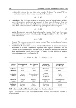

![Engineering Education and Research Using MATLAB270
Usually, the starting point to represent a real system as a Bond Graph diagram are the
sources, in this case a flow source (ground velocity). The next step is to think about the
power flows through the system components, power flows produced by the effort and flow
variables. As figure 3 illustrates the spring and the damper are moved at a velocity that
must be the difference between the mass velocity v1(t) and ground velocity v0(t). This means
that a “0” junction must be used as figure 4 illustrates.
The spring is represented as a compliance bond and the damper as a resistance bond. Both
components move at the same velocity, but each one needs different forces to move at this
velocity. This means that a “1” junction must be used as figure 4 illustrates. Finally, the mass
is represented as an inertia bond that moved at v1(t) velocity. Due to the fact that the system
is under gravity of earth, an effort source must be used.
Bond Graph method calculates the flow and effort on each Bond, and uses as system variables
the displacement associated to compliance (K1) bond [x(t)] and momentum associated to
inertia (m1) bond [P(t)].
SE : -m *g
I : m
f
e
f
e
fe
fe
f
e
f
e
f
e
1
1
1
1
2
2
3 3
4
4
5
5
6
6
7
7
C : K1
R : R1
SF : V0
10
1
Fig. 4. Bond Graph of the one DOF system
According to the Bond Graph showed in figure 4, the flows in each bond are presented in the
equations shown in (11):
1 0
2 1 3 0
1
3 4 5
1
6 7 2 0
1
( )
( )
( )
f V t
P
f f f V t
m
P
f f f
m
P
f f f V t
m
=
= − = −
= = =
= = = −
(11)
The efforts in each bond are presented in the equations shown in (12).](https://image.slidesharecdn.com/engineeringeducationandresearchusingmatlab-160628213608/85/Engineering-education-and_research_using_matlab-280-320.jpg)
![Analysis of Dynamic Systems Using Bond Graph Method Through SIMULINK 271
1 2 3
2 6 7 1 1 0
1
7 1
6 1 0
1
5 2
4 5 3 1 1 0 1
1
( )
( )
( )
e e e
P
e e e K X R V t
m
e K X
P
e R V t
m
e m g
P
e e e K X R V t m g
m
= =
⎛ ⎞
= + = ⋅ + ⋅ −⎜ ⎟
⎝ ⎠
= ⋅
⎛ ⎞
= ⋅ −⎜ ⎟
⎝ ⎠
= − ⋅
⎛ ⎞
= + = ⋅ + ⋅ − − ⋅⎜ ⎟
⎝ ⎠
(12)
That system dynamic behaviour is represented by the following two equations shown in 13
and 14:
7 0
1
( ) ( )
( )
dX t P t
f V t
dt m
= = − (13)
4 1 0 1 1
1
( ) ( )
( ) ( )
dP t P t
e K X t V t R m g
dt m
⎛ ⎞
= = ⋅ + − ⋅ − ⋅⎜ ⎟
⎝ ⎠
(14)
These equations are achieved taking into account that the variation of the momentum is
equal to the effort on the inertia bond, and the variation of the displacement is the flow in
the compliance bond. These are two first order differential equations coupled as a function
of the momentum [P(t)] associated to the inertia and displacement [X(t)] associated to the
spring. These systems can be solved without major problems by using differential calculus.
3. Introduction to Simulink
Simulink is an environment for multidomain simulation and Model-Based Design for
dynamic and embedded systems. It provides an interactive graphical environment and a
customizable set of block libraries that allow to design, simulate, implement, and test a
variety of time-varying systems, including communications, controls, signal processing,
video processing, and image processing.
Simulink is integrated with MATLAB, providing immediate access to an extensive range of
tools that make possible to develop algorithms, analyze and visualize simulations, create
batch processing scripts, customize the modelling environment and define signal,
parameters and test data.
With Simulink, a detailed block diagram of a system can be quickly created, modelled and
maintained using a comprehensive set of predefined blocks. Simulink provides tools for
hierarchical modelling, data management, and subsystem customization, making it easy to
create concise, accurate representations, regardless of your system's complexity. Simulink
software includes an extensive library of functions commonly used in modelling as:
• Continuous and discrete dynamics blocks, such as Integration and Unit Delay
• Algorithmic blocks, such as Sum, Product, and Lookup Table
• Structural blocks, such as Mux, Switch, and Bus Selector](https://image.slidesharecdn.com/engineeringeducationandresearchusingmatlab-160628213608/85/Engineering-education-and_research_using_matlab-281-320.jpg)


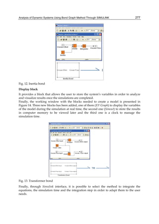


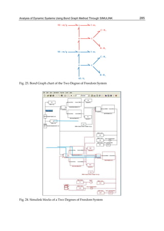


![4 Will-be-set-by-IN-TECH
Weideman and Reddy (2003) or Trefethen (2000), where MATLAB code to generate the
matrices is given.
Discretization of the equation 2 leads to the set of equations
aj,k
M
∑
q=0
(Dxx)j,qψq,k + bj,k
M
∑
q=0
(Dyy)k,qψj,q + cj,k
M
∑
q=0
(Dx)j,qψq,k + ej,k
M
∑
q=0
(Dy)k,qψj,q + fj,kψj,k = gj,k,
(4)
at the interior points 1 ≤ j ≤ M − 1, 1 ≤ k ≤ N − 1. At the boundaries we have ψ = 0.
The discrete set (4) can be combined into a compact form as
[DIAG(a)(IN+1 ⊕ Dxx) + DIAG(c)(IN+1 ⊕ Dx)] Ψ+
DIAG(b)(Dyy ⊕ IM+1) + DIAG(e)(Dy ⊕ IM+1) Ψ + DIAG(f)Ψ = g , (5)
where Ψ denotes the vector of unknowns, A ⊕ B is the kronecker tensor product of two
matrices A, B (which in MATLAB is represented by the kron(A,B) operator), and DIAG(v)
is as in MATLAB the diagonal matrix with entries given by the vector v, and IM+1 is the
identity matrix of order M + 1. Certain rows of the matrix operator in (5) are also modified
when the boundary conditions are incorporated.
The linear sytem may be represented as
SΨ = R. (6)
Once the coefficient matrix S and the right hand sides have been computed, the solution just
involves the use of the operator with Ψ = SR. From the user perspective other than
declaring that the matrices involved are sparse matrices, no additional special treatment is
required to obtain the solution of the linear systems.
Given the discretization matrices, the above system is easy to code in MATLAB. For certain
discretizations however, the linear systems outlined above can be huge and highly sparse.
The bandwidth of the coefficient matrix increases with increasing order of differences used,
and with spectral methods in two directions, the coefficient matrix has the sparsity pattern
similar to that in figure 1(c), obtained using the spy function in MATLAB. On the other hand
by taking second-order finite differences in the x−direction and spectral collocation in the
y−direction, with a particular ordering of grid points, the matrices can be written in block
tridiagonal form as shown in figure 1(a),1(b), or with fourth order finite-differencing in x the
linear system is block pentadiagonal. With 2nd, 4th or even 6th finite-differencing the linear
systems can be solved with a direct solver but with spectral methods in two directions, unless
the differential operator involved has a special form, it is not immediately possible to utilize
the sparse nature of the matrix. Whilst this does not pose any intrinsic difficulties if one is
coding in MATLAB, with increased number of points the solution phase can become very
memory intensive and requires a lot of processor time. The use of the hybrid approach in our
work is motivated in part by the observation that the sparse matrix structure can be exploited
to write efficient solvers, which not only work well with MATLAB, but can be coded directly
in other languages. MATLAB provides for an excellent environment in which one can test and
develop solvers of this type. In our work we have written our own direct block solvers as well
as making direct use of the operator with a sparse matrix.
In the MATLAB codes when constructing the coefficient matrices, we use the functions speye
or spalloc for initially creating the sparse matrices. After this only the non-zero elements of
the matrices are assigned.
292 Engineering Education and Research Using MATLAB](https://image.slidesharecdn.com/engineeringeducationandresearchusingmatlab-160628213608/85/Engineering-education-and_research_using_matlab-302-320.jpg)


![Solving Fluid Dynamics Problems with Matlab 13
Note that a shock point can be seen as an addition of both elliptic and hyperbolic x difference
operators.
In the Y direction, the physical domain was first truncated to y∞ and mapped into the
Chebyshev space, as in Canuto et. all (1998),
Y ∈ [0, y∞] → z ∈ [−1, 1]
where,
zj = cos(
jπ
N
), j = 0, 1, ..., N
and,
Yj = y∞(
zj + 1
2
).
First and second derivatives in the Y directions were calculated as described earlier.
After applying the above discretizations we obtain a set of coupled nonlinear algebraic
equations. These are linearized using Newton-Raphson linearization by setting
ψi,j = ψi,j + Gi,j,
where ψi,j represents the value of ψi,j in a previous iteration and Gi,j represents the update for
ψi,j. This results in a linear system of equations for the Gi,j of the form
Ai,jGi−2,j + Bi,jGi−1,j + Ci,jGi,j + Hi,jGi+1,j + Ei,jGi+2,j = Fi,j. (25)
Details on how to calculate the coefficients Ai,j, Bi,j..., Fi,j can be found in Pereira and Gajjar
(2010). The block pentadiagonal system of equations was solved directly using routines
described in Korolev et all. (2002).
4.2 The use of GUIs
In this subsection we will focus on how to generate a good graphics interface using MATLAB
GUIs in the context of the problem described in the previous subsection. In order to obtain
a graphics interface to our programme, the first thing we have to do is to type guide in
MATLAB’s command window. The result is that MATLAB opens a window that has a
graphics interface working environment(GIWE). The next thing to do, is to save it as name.fig.
This action has as a result not only of saving the work done so far, but also to generate a file
name.m, that has the MATLAB corresponding instructions.
Suppose next that we want to introduce a title on top of the graphics interface window. We
select the "Static text" button in the GIWE. With the mouse one selects the location and the
size of the text to input. Then after double clicking on it a new window appears, where one
can choose options for the static text we want to introduce.
Another important feature on the design of an interface, is how to read data from this interface.
To do so, one option is to select the "Edit text" button in the GIWE. With the mouse one selects
the location and the size of the text to be read. Then, after a double click a new window
appears where one can chose options for the text to be read from the keyboard. It is possible
to choose a default text that can be attributed to a certain variable in the MATLAB code. If we
fill in the field "Tag" with a name, that can be used to attribute the edited text to a variable.
Suppose we fill the field "Tag" with A1. By doing this and saving it, one automatically obtains
301Solving Fluid Dynamics Problems with Matlab](https://image.slidesharecdn.com/engineeringeducationandresearchusingmatlab-160628213608/85/Engineering-education-and_research_using_matlab-311-320.jpg)


![The Use of Matlab in the Study of the Glass Transition and Vitrification in Polymers 317
340 350 360 370 380 390
-0.08
-0.06
-0.04
-0.02
0
Temperature (K)
Cpout-of-phase(J/gK)
b
(b)
340 350 360 370 380 390
-0.08
-0.06
-0.04
-0.02
0
Temperature (K)
Phaseangle(rad)
c
(c)
340 350 360 370 380 390
1.25
1.3
1.35
1.4
1.45
1.5
1.55
1.6
Temperature (K)
Cp,ave(J/gK)
(d)
Fig. 5. Fourier transformed signals (red curves) for modulated cooling curve of Figure 4: (a)
in-phase heat capacity; (b) out-of-phase heat capacity; (c) phase angle; (d) average heat
capacity. In Figure 5a, modulation periods [s] are: 120 (black), 60 (green), 30 (blue), 12 (red),
6 (lilac). In Figure 5d, the cooling rates [K/min] are: −0.5 (green), −1 (red), −2 (blue), −5 (black),
−10 (magenta)](https://image.slidesharecdn.com/engineeringeducationandresearchusingmatlab-160628213608/85/Engineering-education-and_research_using_matlab-327-320.jpg)


![The Use of Matlab in the Study of the Glass Transition and Vitrification in Polymers 323
initially to 1 for the fully cured material, can be described by various different kinetic
equations. One of the most widely used equations is that of Kamal (Kamal, 1974), which
describes an autocatalytic reaction:
( )( )1 2
chem
d
= 1
d
nm
k k
t
α
α α
⎛ ⎞
+ −⎜ ⎟
⎝ ⎠
(10)
where k1 and k2 are temperature dependent rate constants and the exponents m and n are the
reaction orders. The rate constants depend on temperature according to the Arrhenius
equation:
c,1
c,1 1exp
E
k A
RT
⎛ ⎞
= −⎜ ⎟
⎝ ⎠
(11a)
c,2
c,2 2exp
E
k A
RT
⎛ ⎞
= −⎜ ⎟
⎝ ⎠
(11b)
where A1 and A2 are pre-exponential constants, E is the activation energy, and R is the
universal gas constant. In this equation, a subscript c has been added for k and E to indicate
that that these are values for the chemically controlled reaction.
These Equations 10 and 11 are sufficient to describe the kinetics of the cure reaction when it
is chemically controlled, in other words in the absence of vitrification (to be discussed in
detail below), and the predictions of this model can be compared with experimental DSC
data in the form of heat flow as a function of time (for isothermal cure) or as a function of
temperature (for non-isothermal cure). The specific heat flow, HF [W/g] is given by:
d
=
d
HF H
t
α
∞Δ (12)
where ΔH∞ is the total heat of reaction per unit mass [J/g] for a fully cured system. Typical
results which emerge from this model are shown in Figures 7a and 7b for isothermal and
non-isothermal cure, respectively, where the effects of some of the experimental parameters
are included: in Figure 7a, four different isothermal cure temperatures (50ºC, 60ºC, 70ºC and
80ºC) are used, with the reaction occurring at shorter times as the cure temperature
increases; in Figure 7b, four different heating rates are used (1, 2, 5 and 10 K/min), with the
reaction shifting to higher temperatures with increasing heating rate.
By fitting these kinetic equations to the experimental data, it is possible to evaluate the
various kinetic parameters, in particular the activation energies, the pre-exponential
parameters, and the reaction exponents, m and n. In principle, the same parameter values
will be obtained from both isothermal and non-isothermal experimental data. In practice,
however, the kinetic equations are only an approximation to the real situation, which is
generally much more complex, involving not just one reaction, for example the reaction of
the primary amine of the cross-linking agent with the epoxy monomers, but also other
reactions such as the reaction of secondary amines which result from the first reaction, and a
homopolymerization reaction (etherification) which can be catalyzed by the tertiary amines
resulting from the second reaction (Fernández-Francos et al, 2007; Kubisa & Penczek, 1999;
Montserrat et al, 2008; Pascault et al, 2002; Tanaka & Bauer, 1988). The result of this added](https://image.slidesharecdn.com/engineeringeducationandresearchusingmatlab-160628213608/85/Engineering-education-and_research_using_matlab-333-320.jpg)
![Engineering Education and Research Using MATLAB324
complexity is that a best fit to non-isothermal data does not always result in a best fit for the
isothermal data. Nevertheless, in most instances a satisfactory fit can be obtained to all the
experimental data, and the evaluation of the parameter values then provides useful
information about the reaction kinetics.
0 50 100 150 200 250 300
0
0.05
0.1
0.15
0.2
0.25
0.3
0.35
time (min)
HeatFlow(W/g)
a
increasing cure temperature
250 300 350 400 450 500 550
0
0.5
1
1.5
Temperature (K)
HeatFlow(W/g)
bincreasing heating rate
Fig. 7. Cure simulations under isothermal [(a): at 50ºC, 60ºC, 70ºC and 80ºC] and non-
isothermal [(b): at 1, 2, 5 and 10 K/min] conditions. Parameters: m=0.5, n=1.5, A1=103.6 s,
A2=103.4 s, Ec,1=51.8 kJ/mol, Ec,2=41.5 kJ/mol, ΔH∞=520 J/g
The usual procedure for evaluating the parameter values from the experimental data is first
to determine the total heat of reaction, per unit mass of sample, from the non-isothermal
cure curves. This is calculated as the area under the cure curve of heat flow per unit mass of
sample as a function of temperature, normalized by the heating rate. For a stoichiometric
ratio of diglycidyl ether of bisphenol-A (DGEBA) epoxy resin and a diamine curing agent,
for example, this is approximately 400 J/g. The reason for using the non-isothermal cure
rather than the isothermal cure is that in isothermal cure it is possible that vitrification might
occur. If this happens, then the cure does not proceed to completion, but the cure rate
decreases to zero before the reaction is complete, and it is not possible to identify, by
conventional DSC, whether or not this occurs. An analysis of the isothermal cure curve
under these circumstances, using the kinetic Equations 10-12 above, would lead to](https://image.slidesharecdn.com/engineeringeducationandresearchusingmatlab-160628213608/85/Engineering-education-and_research_using_matlab-334-320.jpg)


![Advanced User-Interaction with GUIs in MatLAB® 343
$- executive control statement
SOL 101 $- solver type. "101" corresponds to the linear static solver
CEND
$- case control section
SUBCASE 1 $- sub-case entries
$- beginning bulk data section
BEGIN BULK
…
CQUAD4 104 1 122 123 134 133
$- element quad id=104, material id=1, connected nodes: 122,123,134,133
CTRIA3 105 1 150 151 152
$- element tria id=105, material id=1, connected nodes: 150,151,152
…
GRID 150 0.0 0.0 1.0 5
$- node id=150, coordinates [0.0, 0.0, 1.0], local UCS id=5
…
SPC 1 176 1 0.00
$- define single point constraint
…
PWELD 1 3 5.00
…
CWELD 1 1 ALIGN 125 9
$- cweld element to define fasten elements
….
FORCE 1 9 2 10.54 0.00 0.00 1.00
$- define load conditions
…
CORD2R 5 80.00 0.00 4.00 80.00 0.00 5.00 79.00 0.00 4.00
$- define local coordinate UCS
…
ENDDATA
$- ending bulk data file
When importing mesh data from .bdf formatted files, no geometric information is available
about connected domains. We implemented an automatic procedure allowing to select and
store connected domain. Every connected domain corresponds to a part, which can be
introduced into the assembly process being simulated.
The general idea to extract connected domains is to consider the imported mesh as a graph
in which mesh elements correspond to graph-vertices, while each edge represents an
element-to-element connection (see Annex A.2 for a general overview on the main concepts
of the Graph Theory used in the application). Looking at Fig. 5, 9 elements (five CQUAD4
and four CTRIA3) define two connected domains: (I, III, V, VI, IX) and (II, IV, VII, VIII). The
graph representation depicted into Fig. 5b was obtained considering that two elements are
connected if they share one edge or one node. For example, element I is connected to
element IX, through one edge, and to elements III and VI, with one node.
Starting from the definition provided into equation (A.2), the adjacency matrix, "A", of the
mesh-graph can be easily calculated. Knowing the adjacency matrix (Nquad+Ntria x
Nquad+Ntria square matrix, where Nquad and Ntria are, respectively, the number of imported
CQUAD4 and CTRIA3 elements), a growing procedure can be applied to detect all
connected domains. Below the MatLAB®'s pseudo-code.](https://image.slidesharecdn.com/engineeringeducationandresearchusingmatlab-160628213608/85/Engineering-education-and_research_using_matlab-353-320.jpg)
![Engineering Education and Research Using MATLAB344
%- find-out connected domains
function domain=connectedDomain(A)
seed=1;
while true
idConnect=[];
visited(seed)=true; %- seed has been already visited
for i=1:length(seed) %- loop over seed elements
%- get connected elements by using "A" matrix
[temp,visited]=getConnected(seed(i),A,visited);
idConnect=[idConnect,temp];
end
%- "local domain"
tempDomain=[tempDomain,idConnect];
if ~isempty(idConnect)
%- update seed counter
seed=idConnect;
else
%- if no connected element is found then save "local domain"
count=count+1;
domain{count}=tempDomain; %- new domain counted
%- look for a new seed (not yet visited)
seed=getNotVisited(visited);
tempDomain=seed;
end
%- break loop when there is no new seed (all elements were allocated)
if isempty(seed)
break
end
end %- end loop
The procedure looks for those elements connected to the initial "seed element". Thus,
iteratively, the seed counter is update with the so-connected elements ("idConnect"). When
no other connected element is counted, then a connected domain has been selected and it is
saved. These connected elements are classified as "visited". The iterative procedure stops
when all elements have been marked as visited. Once connected domains are calculated,
SVA-FEA updates its data structure: "ELEMENT.Quad", "ELEMENT.Tria" and "NODE"
fields are filled, accordingly, with respect to the i-th connected domain (see Fig. 4). The
"patch" MatLAB® built-in function is used to draw and visualize mesh data.
2.3 SVA-FEA software: selecting mesh nodes
Many efforts were done to make the SVA-FEA's GUI friendly as much as possible. In
particular, when fixture or fasten points have to be assigned, the easiest way is just to select,
by mouse picking, mesh node from the graphic area.
This task can be accomplished by using MatLAB® graphic tools. Fig. 6 reports the general
scheme adopted in MatLAB® for defining a scene (MatLAB® supports both parallel and
perspective projections; however, the actual implementation of SVA-FEA supports only the
parallel projection).](https://image.slidesharecdn.com/engineeringeducationandresearchusingmatlab-160628213608/85/Engineering-education-and_research_using_matlab-354-320.jpg)

![Engineering Education and Research Using MATLAB346
%- transform mesh-nodes, "Ncoord"
Ncoord=R*Ncoord';
Pmi=R*Pmi';
%- take just (x-y) components
Ncoord= Ncoord(1:2,:);
Pmi=Pmi(1:2);
%- calculate distances
diff=[Ncoord(1,:)-Pmi(1); Ncoord(2,:)-Pmi(2)];
dist=sqrt(sum(diff.^2,1));
%- finally, find-out the index related to the minimum distance
[~,idSelected]=min(dist); %- discard (~) first output
(a) drawing rectangle by mouse picking/moving (b) selecting mesh-nodes
Fig. 7. Application of the rectangle-area selection algorithm
The algorithm just described can be extended to allow rectangle-area selection from the
graphic area by defining three sub-routines running when picking mouse buttons or moving
mouse into the current MatLAB® figure. The procedure can be summarized as follows (see
also Fig. 6):
• calculating "Pm1" point and "R" matrix when picking down the mouse button
("WindowButtondownFcn" callack);
• calculating "Pm4" point and draw rectangle-area selection when moving the mouse
("WindowButtonMotionFcn" callack); and,
• calculating mesh-nodes inside the rectangle-area selection ("WindowButtonUpFcn"
callack).
"Pm1" is calculated once picking down the mouse button. "Pm4" corresponds to the actual
position of the mouse cursor. The MatLAB® pseudo-code is reported below.
The "patch" and "line" MatLAB® built-in functions are used to draw, respectively, the
rectangle-area selection and the selected mesh nodes. Furthermore, the "inpolygon"
MatLAB®'s command is here adopted to check which nodes are inside the rectangle-area.
As example, in Fig. 7 a mouse selection is drawn into the upper side of figure (Fig. 7a). Then,
the selected mesh nodes are marked as blue dots (Fig. 7b).](https://image.slidesharecdn.com/engineeringeducationandresearchusingmatlab-160628213608/85/Engineering-education-and_research_using_matlab-356-320.jpg)
![Advanced User-Interaction with GUIs in MatLAB® 347
%- inizialize selection phase:
set(fig,'WindowButtondownFcn',{@sClick,Ncoord});
function sClick(Ncoord)
%- built frame
R=[Xc;Yc;Zc];
%- start selection
P1=get(gca,'CurrentPoint'); %- picked point
%- start mouse motion
set(gcf,'WindowButtonMotionFcn',{@moveMouse,P1,R,Ncoord})
function moveMouse(P1,R,Ncoord)
%- actual mouse position
P4 = get(gca,'CurrentPoint');
%- transform into the local frame
P1=R*P1';
P4=R*P4';
%- built rectangle selection
P2=[P1(1) P4(2) 0];
P3=[P4(1) P1(2) 0];
%- go-back into global frame
Vertext=R'*[P1;P2;P4;P3];';
%- draw rectangle
patch('Faces',[1 2 3 4],...
'Vertices',Vertext');
%-call mouse button-up
set(fig,'WindowButtonUpFcn',{@endClick,R,Ncoord,Vertex});
function endClick(R,Ncoord,Vertex)
inPol=inpolygon(Ncoord(1,:),Ncoord(2,:),Vertex(:,1),Vertex(:,2));
Psel=Ncoord(inPol,:);
line('xdata',Psel(:,1),...
'ydata',Psel(:,2),...
'zdata',Psel(:,3))
In SVA-FEA, when defining fasten or contact points, mesh-nodes are directly selected from
the graphic area (see Fig. 8) by using the rectangle-area selection tool. Once master and slave
parts are picked, matched nodes are automatically assigned among parts. After selecting
master node, the related matched node is calculated as the nearest one on the slave part. In
Fig. 8, matched nodes are marked as circle dots.
2.4 SVA-FEA software: Tree view implementation
Imported connected domains and KPs can be edited and managed thought the MODEL
TREE, serving as tree viewer (see Fig. 9). Specific programming languages, such as](https://image.slidesharecdn.com/engineeringeducationandresearchusingmatlab-160628213608/85/Engineering-education-and_research_using_matlab-357-320.jpg)

![Advanced User-Interaction with GUIs in MatLAB® 349
(a) collapsed MODEL TREE (b) expanded MODEL TREE
Fig. 9. MODEL TREE visualization
function testListbox
%- define a new figure
fig=figure('unit','characters','position',[20 5 160 45]);
%- define a listbox
hList=uicontrol('unit','characters','Style','listbox',...
'position',[0 0 35 45],...
'parent',fig,'enable','on');
%- set call-back function
set(hList,'callback',@listCall)
%- call-back function handling
function listCall(src,event)
%- differentiate depending on "SelectionType" property
if strcmp(get(gcf, 'SelectionType'), 'open') %- double-click
set(src,'string','OPEN','value',1)
elseif strcmp(get(gcf, 'SelectionType'), 'normal') %- single-click
set(src,'string','NORMAL','value',1)
end
Based on this key feature, the MODEL TREE was implemented in SVA-FEA to manage and
visualize the modeling history. When importing new part or defining new KPs, the MODEL
TREE is automatically updated. As example, Fig. 9 shows the MODEL TREE in which one
can browse among part options (PART) and KPs (UCS, CONSTRAINT, CONTACT,
FASTEN, MEASURE). Right-mouse-clicking was also programmed to allow a fast editing of
the selected item.
2.5 SVA-FEA software: Assembly tree implementation
A crucial aspect to be achieved when performing the variation analysis of compliant parts is
the assembly sequence, that is the sequence through which parts or sub-assemblies are put](https://image.slidesharecdn.com/engineeringeducationandresearchusingmatlab-160628213608/85/Engineering-education-and_research_using_matlab-359-320.jpg)


![Engineering Education and Research Using MATLAB358
//… routine code…
}
double userfnc#2(…)
{
//… routine code…
}
// GATEWAY ROUTINE SECTION
void mexFunction(int nlhs, mxArray *plhs[], int nrhs,
const mxArray *prhs[])
// nlhs = number of output items
// nrhs = number of input items
// plhs = output pointers
// prhs = input pointers
{
// get pointer from MatLAB® input
A = mxGetPr(plhs[…]);
// create MatLAB® variable
plhs[…] = mxCreateDoubleMatrix(…);
// allocate output variable
userfnc(…);
}
The name of the gateway function is always “mexFunction”. This function parses all
MatLAB® inputs into pointer variables (“mxGetPr”) and create the output MatLAB®
variables (“mxCreateDoubleMatrix”). Assuming "testmex.c" is the source code file, the
following line should be written to compile it from MatLAB® (for 64bit MatLAB®
distributions the Microsoft® Visual C++ compiler is suggested by MathWorks; how to
install the Microsoft® Visual C++ for MatLAB® can be found in (Baker, 2009)).
%- link and compile mex source code
mex testmex.c
Therefore, one can now write a MEX file which creates the A array. The source C++ code of
the "testmex.c" file is something like this:
#include "mex.h"
// computational routine
void allocateArray(double A[], int nr)
{
int i; // locale variable
for (i=0; i<nr; i++){
A[i]=i+1; // "fill" array
}
}
// gateway routine
void mexFunction(int nlhs, mxArray *plhs[], int nrhs,
const mxArray *prhs[])
{](https://image.slidesharecdn.com/engineeringeducationandresearchusingmatlab-160628213608/85/Engineering-education-and_research_using_matlab-368-320.jpg)
![Advanced User-Interaction with GUIs in MatLAB® 359
double *A; // pointer to “int” type
int nr; // define “int” variable
// get “int” value from the input pointer
nr = (int)*mxGetPr(prhs0]);
// allocate MatLAB® double matrix
plhs[0] = mxCreateDoubleMatrix(nr,1, mxREAL);
// get the pointer to the output
A = mxGetPr(plhs[0]);
// allocate the output array by using the computational routine
allocateArray(A,nr);
}
The compiled function may be easily called from MatLAB®, typing:
%- use compiled function
A=testmex(N);
The elapsed run-time is now 0.2893 s, that is, about 70% faster than the previous MatLAB®
script. This way is particularly useful when managing large data sets, or nested loops are
required.
A.2 Adjacency matrix and Laplace matrix
A graph "G" is usually defined by means of the vector list of vertices, "V", and the edge
matrix, "E" (Berge, 2001; Deo, 2004).
3
2
1
4
5
3
2
1
4
5
(a) not-oriented graph (b) oriented graph
Fig. A.1. Graph representation
"V" is a vector of integer ranging from 1 to Nv, where Nv is the total number of vertices. "E"
is an Nex2 matrix, in which the i-th row has the indices of vertices connected by that edge
(Ne is the number of edges). Let (i, j) be the couple of entries on the i-th row. For not-
oriented graphs (see Fig. A.1a) it is (i, j)=(j, i), whereas (i, j)≠(j, i) for oriented graphs (see Fig.
A.1b). Moreover, the same couple of vertices may be connected with more than one edge (in
Fig. A.1, vertices 1 and 3 are connected with 2 edges).](https://image.slidesharecdn.com/engineeringeducationandresearchusingmatlab-160628213608/85/Engineering-education-and_research_using_matlab-369-320.jpg)


![4 Will-be-set-by-IN-TECH
complete equations (e.g. as a function) into MATLAB. For example, for the case of a four
layered structure (layers indexed by i, j, k, l) this would be:
r
P(S)
ijkl =
r
P(S)
ij + r
P(S)
jkl exp[2i(εjμj(εiμi)−1 − u2)
1
2 kidj]
1 + r
P(S)
ij r
P(S)
jkl exp[2i(εjμj(εiμi)−1 − u2)
1
2 kidj]
(2)
with
r
P(S)
jkl =
r
P(S)
jk + r
P(S)
kl exp[2i(εkμk(εiμi)−1 − u2)
1
2 kidk]
1 + r
P(S)
jk r
P(S)
kl exp[2i(εkμk(εiμi)−1 − u2)
1
2 kidk]
(3)
and
rS
ij =
μj(1 − u2)1/2 − μi[εjμj(εiμi)−1 − u2]1/2
μj(1 − u2)1/2 + μi[εjμj(εiμi)−1 − u2]1/2
(4)
rP
ij =
εj(1 − u2)1/2 − εi[εjμj(εiμi)−1 − u2]1/2
εj(1 − u2)1/2 + εi[εjμj(εiμi)−1 − u2]1/2
(5)
where εi, μi and di are the permittivity, permeability and thickness of the ith layer. The
total wavevector in the ith layer is given by ki =
√
εiμiω/c where ω is the frequency of
the electromagnetic field and c is the speed of light in vacuum. Also a normalized in plane
wavevector is defined as u = kx/k1, where kx is the in plane wavevector component which is
independent of the layer. The value of ε for the metal will in general be complex and frequency
dependent, and is most easily obtained by fitting a high order polynomial to experimentally
measured data (e.g. Drachev (2008) for silver). Alternatively for not to thin metal layers
one may to a good approximation use a Drude-Sommerfeld model (e.g. Kittel (1995)) where
the parameters can later be systematically varied to account for e.g. changes in temperature
Elsayad and Heinze (2010b).
To determine the dispersion relation and the cut-off energy of a given structure one may
also make use of the natural matrix calculation approaches of MATLAB. To do so one firstly
writes a general expression for the parallel electric fields in each layer. For a layer-i extending
from z = zmin to z = zmax this would be A
(1)
i ekzi(z+zmin) + A
(2)
i e−kzi(z+zmax), where kzi is the
out of plane wavevector in the layer and A
(1)
i & A
(2)
i are at this point arbitrary complex
coefficients. One may then write the corresponding magnetic induction fields for each layer
using Maxwell’s equations (i.e. by taking the normal derivative), so that for each layer one
has two equations with two unknowns. This is done for each layer i = 1, 2...N. Finally
one constructs a 2N × 2N with the coefficients for each layer constituting the entries in
each row. The determinant of this matrix will then give the dispersion relation ω(kx) - see
e.g. Dionne et al. (2008). Since kx is complex one can not simply assign a solver such as
fzero to the task. It is it turns out often necessary to evaluate this by brute force - i.e.
letting MATLAB evaluate the determinant for a given complex transverse wavevector and
checking how close it is to zero. In general it is important to provide a good starting guess
of Re(kx) and Im(kx) for each frequency. For the cases of interest, where the frequencies of
interest are close to the cut-off frequency, a good starting guess for the former is the light-line
Re(kx) = nω/c of the medium with refractive index n in which the mode becomes unbound,
366 Engineering Education and Research Using MATLAB](https://image.slidesharecdn.com/engineeringeducationandresearchusingmatlab-160628213608/85/Engineering-education-and_research_using_matlab-376-320.jpg)
![Using MATLAB to Achieve Nanoscale Optical Sectioning in the Vicinity of Metamaterial Substrates by Simulating Emitter-Substrate Interactions 5
and then to progressively search further into the evanescent region, i.e. Re(kx) = nω/c + δ
with δ ∼ 0.01nω/c. For the imaginary part Im(kx) - which diverges at the cut-off - it is most
efficient to employ an algorithm which calculates the gradient of the determinant between
two nearby values of Im(kx) [i.e. taking the difference in the determinant value and dividing
by the difference in Im(kx)], and subsequently search for larger/smaller Im(kx) values if the
determinant is smaller/larger than zero. The stability of the solution should be checked
to assure Limδ→0{ω(kx + δ) − ω(kx − δ) → 0}. The above mentioned approach typically
requires that Im(kx) is well behaved and monotonous in the vicinity of the cut-off, which is
fortunately often the case. Since the equation has to be satisfied for both Re(kx) and Im(kx)
optimizations of both of these have to be performed simultaneously. For completeness an
analysis can also be performed for transverse electric (TE) as well as transverse magnetic
(TM) polarizations, although for the cases of the very thin non-magnetic plasmonic structures
only the latter are usually relevant. For the case of highly asymmetric structures of few
layers, coupling between the interfaces may be negligible and a single plasmonic mode at
one interface can to a good approximation be assumed solely responsible for the dispersion
of the cut-off mode Burke and Stegeman (1986). In this case the cut-off energy can for a
non-magnetic structure be estimated by Ec = ¯hcεjεk[εi(εj + εk)]−1, where εi is the permittivity
of the medium where the cut-off occurs, and εj and εk are the permittivities on either side of
the interface at which the mode is originally localized.
The principle of MeSuMo requires that the cut-off of the structure falls within the emission
spectrum of the emitter. Since many common fluorophores and dyes have a fairly broad
emission spectrum this criteria can usually be met quite easily and is generally quite robust.
To calculate the change in intensity at a given frequency one firstly defines the change in
the decay rate of a fluorophore as a function of distance and frequency. This may (at not
too small distances) be modeled quite well in the dipole approximation using the classical
Chance-Prock-Silbey (CPS) model Chance (Prock and Silbey). Under these conditions the
decay rate in the +ˆz and −ˆz direction (away from and towards the substrate respectively)
for perpendicular (⊥) and parallel (||) electric dipole like emitters can be obtained by:
ˆΓ⊥
+ = q −
3q
4
Im
1
0
(I1 + I2) du
ˆΓ⊥
− =
3q
4
Im
1
0
I1du −
∞
1
I2du (6)
ˆΓ
||
+ = q −
3q
8
Im
1
0
(I3 − I4)du
ˆΓ
||
− =
3q
8
Im
1
0
I3du +
∞
1
I4du (7)
in which the integrands are
I1 = 2u3 1 − |rP|2
(u2 − 1)
1
2
I2 = u3 rP
(u2 − 1)
1
2
exp[2(u2
− 1)
1
2 k1z]
I3 = u
(1 − |rS|2) + (1 − u2)(1 − |rP|2)
(u2 − 1)
1
2
I4 = 2u
rS + (1 − u2)rP
(u2 − 1)
1
2
exp[2(u2
− 1)
1
2 k1z] (8)
367
Using MATLAB to Achieve Nanoscale Optical Sectioning
in the Vicinity of Metamaterial Substrates by Simulating Emitter-Substrate Interactions](https://image.slidesharecdn.com/engineeringeducationandresearchusingmatlab-160628213608/85/Engineering-education-and_research_using_matlab-377-320.jpg)
![6 Will-be-set-by-IN-TECH
where q is the quantum yield of the emitter, the superscripts P(S) denote the transverse
electric(magnetic) cases, and the z and ω dependence of ˆΓ
⊥(||)
+(−)
is implied. The integrals can in
most cases quite easily be evaluated numerically (e.g. using quad). It may be the case that the
structures have resonances (as can be determined by plotting the integrands as a function of
u), in which case one may want to re-write the integrals to assure one integrates in a complex
plane around them and account for the pole(s) in the conventional fashion. Integration can in
almost all cases safely be cut-off at u ∼ 1000, with the contribution beyond u ≈ 100 becoming
negligibly small for z > 10nm. In what follows we will sometimes make use of the notation
Γij = 1
3 [(Γ⊥
+ + Γ⊥
−) + 2(Γ
||
+ + Γ
||
−)]ωij
to signify the isotropic average total decay rate from state
i to j separated in energy by ωij = ωi − ωj. The energy dependence of Γij is understood to be
contained in rS,P = rS,P(ωij), u = u(ωij) and k1 = k1(ωij).
Besides the modification in the decay rate which has been described above, the measured
emission intensity of an emitter will also depend on it’s excitation rate. In particular the
measurable emission intensity for the transition from the excited state a to a lower state b,
which corresponds to a wavelength λab = 2πc/ωab will be given by:
I(ωab) ∝ | ˆμa · Eex(ωab)|2
fabΓR
abΓ−1
a (9)
where Eex(ωab) is the excitation field at the frequency ωab, and ˆμa is the dipole moment of the
excited state a. ΓR
ab and Γa are the radiative decay rate for the transition a → b and the total
decay rate of the state a. fab is the Franck Condon coefficient between a and b, which is related
to the rotational and vibrational configurations of the two energy states relative to each other,
and can be thought of as the intrinsic favourability of the transition. For a realistic emitter
there will in general be many other significant “down transitions” originating from the same
excited state. For the decay of the state a to any other state x, one may thus write:
I(ωax) =
fax
fab
ΓR
ax
ΓR
ab
I(ωab) (10)
Subsequent decay of all states x (and state b) to a common ground state is assumed to proceed
non-radiatively and at a rate several orders of magnitude larger than the radiative decay
rate. For the case of spontaneous emission we consider it can for all intense and purposes be
assumed to be instantaneous. If we neglect direct resonant energy transfer between emitters
(i.e. assume sufficient dilution), then the total excitation field with a frequency ωab at the
location of the fluorophore will be the sum of the external incident field E0(ωab), the reflection
of this field from the structure re−2(1−u2
)1/2
k1zE0(ωab) where r is the reflection coefficient, and
the field generated from excitations in the material by all the fluorophores Er(ωab, z), i.e.
Eex(ωab, u, z) = [1 + re−2(1−u2
)1/2
k1z
]E0
(ωab) + Er(ωab, u, z) (11)
The polarization for the reflected field can in most cases be taken as that of the incident
excitation field. For the case of a single fluorophore Er(ωab, z) is given by the integrands
of equations (6) and/or (7), which are identical to the reflected field for a given transverse
wavevector component u, and will henceforth be written as E0
r (ωab, u, z). To calculate the
reflected field from all of the fluorophores at various distances from the substrate one can
368 Engineering Education and Research Using MATLAB](https://image.slidesharecdn.com/engineeringeducationandresearchusingmatlab-160628213608/85/Engineering-education-and_research_using_matlab-378-320.jpg)
![Using MATLAB to Achieve Nanoscale Optical Sectioning in the Vicinity of Metamaterial Substrates by Simulating Emitter-Substrate Interactions 7
proceed in several ways. It is of no practical relevance in our applications if one requires
information on the position and orientation of each and every contributing fluorophore. We
thus can proceed only via an effective medium approximation. We will assume a density ρ of
fluorophores which may only vary in the axial (z) direction. In the case for ρ(0 < z < zmax) =
ρ and ρ(z > zmax) = 0 one obtains by integrating over z ={0, ∞}:
Er(ωab, u, z) = (1 − e−(1−u2
)1/2
k1zmax
)
ρ
(1 − u2)1/2k1
Γab(u, z)
Γa(z)
E0
r (ωab, u, z/2). (12)
Alternatively one may represent the contribution from a collection of fluorophores by
assigning a negative imaginary response function to the top layer (layer-1) in which they are
immersed - i.e. set Im(ε1)< 0 for non-magnetic structures. Whilst this may be computationally
simpler for constant densities, for the case of a non-trivial z dependence the calculations
become significantly more elaborate. We thus proceed with the former method.
For imaginary (1 − u2)1/2k1 the coupling fields are propagating and equation (12) can be
reduced to the result for e.g. the field in a large semi-transparent 1D box filled with emitters.
For real (1 − u2)1/2k1 the field will on the other hand decay rapidly with increasing z as one
would expect. The contribution to I(ωab) from equation (12) will in itself however only be
small even for large ρ (> 0.01nm−1).
There will be an additional second order contribution to the excitation field and hence the
emission intensity at ωab from excited surface modes of energy ωax where x = b. This
contribution is only significant because the SPP modes have very short decay times - typically
Γ ∼ O(10-100fs), such that their uncertainty broadening is relatively large - O(1 − 10eV). For
ωax ∼ ωab, or more specifically |ωax − ωab| ∼ O(meV), they will contribute significantly
to ER(ωab, z). It follows that when the energy ωab corresponds to mainly real values of
(1 − u2)1/2k1 (evanescent fields) whereas ωax to mainly imaginary values of (1 − u2)1/2k1
(propagating fields) this contribution becomes large near the surface as fluorophores far away
from the substrate can effectively pump those nearby. To the lowest order the contribution
can be written as:
E0
r (ωax, u, z) = dωα dωβ faβ
Γaβ(u, z)
Γaβ
LaβEr(ωaβ, u, z)Lβαδ(ωα − ωax) (13)
where
Laβ =
1
2π
Γaβ(u, z)
(ωa − ωβ)2 + [Γaβ(u, z)/2]2
(14)
and Γab(u, z) and Er(ω, u, z) are the corresponding values of the total decay rate and reflected
field as a function of transverse wavevector [i.e. the integrands of equations (2) and (2) &/or
(3)]. We note that equation (13) accounts for the energy overlap between a state of energy
ωb and a continuum of states whose energy is given by the dummy variable ωβ. The ωα
integration is performed over a range of frequencies in the vicinity of the cut-off (typically
corresponding to a wavelength range of 30-80nm), over which the energy range coincides
with the emission spectrum of the fluorophore (i.e. are allowed transitions for the particular
fluorophore). The weighting (Franck Condon) factors fαβ are empirically determined from
369
Using MATLAB to Achieve Nanoscale Optical Sectioning
in the Vicinity of Metamaterial Substrates by Simulating Emitter-Substrate Interactions](https://image.slidesharecdn.com/engineeringeducationandresearchusingmatlab-160628213608/85/Engineering-education-and_research_using_matlab-379-320.jpg)
![8 Will-be-set-by-IN-TECH
the emission spectrum of an isolated fluorophore scaled so that the value at ωab it is unity.
We note that it is usually practical or necessary to convert this integration into a discrete sum
with an energy spacing of Δω ∼ 1meV. Information particular to the type of fluorophore (e.g.
energy level positions/separations and corresponding Franck Condon coefficients) may be
implemented when constructing the summation.
Since we will not focus on single molecule studies we assume an isotropic average of dipole
orientations for all cases. This can most easily be done by setting Eiso
R = (1/3)E⊥
R + (2/3)E
||
R
and/or Γiso = (1/3)Γ⊥ + (2/3)Γ|| as appropriate. We also note to calculate the final
measurable emission intensity the integral for ΓR which appears in equations 9 & 10 (and
is given by equations 6 & 7) should only be performed up to
√
εi·NA, where NA is the
numerical aperture of the measuring objective. It is possible to now predict the change in the
measurable emission intensity for arbitrary z and fluorophores, near a metamaterial structure.
In figure 1 we outline the basic backbone of a program that calculates the matrix enhan(j,i)
which quantifies the measurable fluorescence enhancement at discrete distances (index j)
and wavelengths (index i). The order of computations (top to bottom) is such that several
independent calculations can depending on available resources be performed in parallel. The
calculation is performed over all transverse wavevectors up to at least |u| ∼ 10z−1 and
summed at the end (with the corresponding weighting factors to mimic integration).
z-range z(j)
j=1,2..100
normalize & fit
determine ω(ab)
and ω range
structure
(d1,epsilon1,
mu1, etc.)
calculate cut-off energy ω(c)
define Ω(i), i=1,2...10 in vicinity of ω(ab) and ω(c)
calculate reflection coefficients
calculate (12)-(14)
fluorophore
density rho
calculate (11)
excitation field
calculate decay rates
calculate total enhancement for Ω(i)
total enhancement matrix as function of z(j) and Ω(i)
enhan(i,j)
define reflection coeff. & decay rates
i+1
j+1
fluorophore emission
& absorption spectrum metal
dispersion
Fig. 1. Structure of program for calculating a matrix that predicts fluorescence enhancement
We now show how to implement equations 6 &7 (with the integrands defined by equation 9)
in MATLAB, which are required for solving equation 10. To focus on the most relevant part
of the code, we expect the reader to have some familiarity with basic MATLAB programming
syntax (i.e. definition of functions and vector-based MATLAB notation). An example code for
calculating the reflection coefficients [2 - 5] and subsequently performing the integration may
look like:
370 Engineering Education and Research Using MATLAB](https://image.slidesharecdn.com/engineeringeducationandresearchusingmatlab-160628213608/85/Engineering-education-and_research_using_matlab-380-320.jpg)
![Using MATLAB to Achieve Nanoscale Optical Sectioning in the Vicinity of Metamaterial Substrates by Simulating Emitter-Substrate Interactions 9
Listing 1. Numerical integration
1 function main()
2 % -- material permittivities
3 sio2 = 2.13; glass = 2.46;
4 water = 1.78; si3n4 = 4.15;
5 % -- ranges for frequency & wavevectors
6 w_vec = 0 : 0.01 : 4;
7 kx = 0 : 0.000001 : 0.02*pi;
8
9 % -- permittivities & permeabilities &
10 % -- thicknesses for each layer
11 mu = [1 1 1 1];
12 d = [1e6 15 15 1e6];
13 e = [ sio2 permitivity_silver(w,d(2)) si3n4 glass];
14
15 % -- integrate Integrand_1
16 lower = 0; % limits for integrals
17 upper = 1;
18 b_up_a = quad(@(u) integrand_I1(u),lower,upper) );
19
20 function [I1] = integrand_I1(u)
21 [r_S,r_P] = r_1234_vec = r_1234_PS(u,’P’);
22
23 A = 1 - abs(r_P).^2;
24 B = sqrt(u.^2 - 1);
25 I1 = 2.*u.^3.*A./B;
26 end
27
28 function r_1234 = r_1234_PS(u,polariz)
29 global d; global e; global k; global mu;
30
31 exp_term = exp(2i.*sqrt(e(2).*mu(2).*(e(1).*mu(1)).^(-1)-u.^2).*k(1).*d(2));
32 r_12_P = r_ij_PS(u,1,2,"P");
33 r_12_S = r_ij_PS(u,1,2,"S");
34 r_234_P = r_234_PS(u,"P");
35 r_234_S = r_234_PS(u,"S");
36
37 switch(polariz)
38 case {"P"}
39 num = r_12_P + r_234_P.*exp_term;
40 den = 1 + r_12_P .* r_234_P.*exp_term;
41 r_1234 = num ./ den;
42 case {"S"}
43 num = r_12_S + r_234_S.*exp_term;
44 den = 1 + r_12_S .* r_234_S.*exp_term;
45 r_1234 = num ./ den;
46 end
47 end
48
49 function r_234 = r_234_PS(u,polariz)
50 global d; global e; global k; global mu;
51
371
Using MATLAB to Achieve Nanoscale Optical Sectioning
in the Vicinity of Metamaterial Substrates by Simulating Emitter-Substrate Interactions](https://image.slidesharecdn.com/engineeringeducationandresearchusingmatlab-160628213608/85/Engineering-education-and_research_using_matlab-381-320.jpg)
![10 Will-be-set-by-IN-TECH
52 exp_term = exp(2i.*k(1).*d(3).*sqrt(e(3).*mu(3).*(e(1).*mu(1)).^-1-u.^2));
53
54 switch(polariz)
55 case {"P"}
56 r_23_P = r_ij_PS(u,2,3,"P");
57 r_34_P = r_ij_PS(u,3,4,"P");
58 num = r_23_P + r_34_P.*exp_term;
59 den = 1 + r_23_P .* r_34_P.*exp_term;
60 r_234 = num ./ den;
61 case {"S"}
62 r_23_S = r_ij_PS(u,2,3,"S");
63 r_34_S = r_ij_PS(u,3,4,"S");
64 num = r_23_S + r_34_S.*exp_term;
65 den = 1 + r_23_S .* r_34_S.*exp_term;
66 r_234 = num ./ den;
67 end
68 end
69
70 function r_ij = r_ij_PS(u,i,j,polariz)
71 global e; global mu;
72
73 A = (1 - u.^2).^0.5;
74 B = ( e(j).*mu(j).* (e(i).*mu(i)).^-1 - u.^2).^0.5;
75
76 switch(polariz)
77 case {"S"}
78 num = mu(j).*A - mu(i).* B;
79 den = mu(j).*A + mu(i).* B;
80 r_ij = num ./ den;
81 case {"P"}
82 num = e(j).*A - e(i).* B;
83 den = e(j).*A + e(i).* B;
84 r_ij = num ./ den;
85 end
86 end
3. Fitting the experimental data to the model
Data can be acquired using a standard scanning epifluorescence microscope with a
spectrometer and photomultiplier tubes. It is generally most practical to save images as .lsm
files which can be directly read into MATLAB [In our setup each file contains a scanned image
of the sample at ten different wavelengths (e.g. bins centered at λ = 490nm, 500nm, 510nm,
etc.)]. For dynamic studies images at different time intervals can also be stored in a single
.lsm file. Many spectrometers come with MATLAB drivers which allow for acquisition
to also be controlled easily through MATLAB. Else for real time (video type) imaging it is
necessary to save the data incrementally into a directory accessible to MATLAB. The spectral
profile of the fluorophores of interest on an uncoated substrate immersed in a similar refractive
index medium as the actual samples should also be available. The area under this spectrum
should be normalized and extrapolated to a discrete matrix [e.g. fitted to a high order
372 Engineering Education and Research Using MATLAB](https://image.slidesharecdn.com/engineeringeducationandresearchusingmatlab-160628213608/85/Engineering-education-and_research_using_matlab-382-320.jpg)
![Using MATLAB to Achieve Nanoscale Optical Sectioning in the Vicinity of Metamaterial Substrates by Simulating Emitter-Substrate Interactions 11
polynomial and evaluated at the discrete wavelengths indexed by i], and saved as a 1 × 10
matrix Ilambda0(i).
Data analysis is performed on a pixel by pixel basis. For each pixel the spectrum
area is normalized, fitted with a high order polynomial, evaluated at i discrete
wavelengths, and written into a 1 × 10 matrix data(i). The ratio enhanobserved(i)
= data(i)/Ilambda0(i) is then calculated. A 1 × j matrix zn(j) is defined which will
represent the fraction of the emitters in the studied area at a distance corresponding to the
index j from the interface. The task is now to solve enhan*zn-enhanobserved=0, which
is in principle straight forward using a function such as e.g. linsolve. The result is best
presented in a plot of zn as a function of z for each or a collection of pixels, which will show
the distribution of fluorophore distances from the substrate at this particular lateral position.
Depending on the sample studied and the information of interest this may be fitted with a
suitable distribution function to obtain an average and spread in distances of emitters from
the substrate within the analyzed region.
4. Optimizing the model and code
In many cases the initial fluorophore-concentration, metamaterial or coupling parameters
may not be the best or correct parameters for the fit. This is usually evident when the results
show an unexpected distribution for zn. Distances less than 10nm should be ignored as
the approximations of the models (dipole approximation and local dielectric functions) are
no longer valid at such small distances. The most significant source of uncertainty is the
predefined and assumed constant value of the fluorophore concentration rho. To account
for this one may redefine rho as being proportional to the integrated area of zn over z, and
repeat the calculation of zn. Also to account for an axial variation in rho - as would be relevant
for samples where the fluorophore density varies strongly with distance z - one may define
rho(j) = rho*(a + zn(j)/norm(zn)), where a is normalization constant chosen so
that on summation over the distances (i) one recovers the total intensity. In this case all
subsequent calculations have to explicitly account for the additional distance dependence in
rho (j), which significantly increases the computational time. This may be efficiently achieved
by defining rho(j) in a smaller parameter space indexed by n that corresponds to dividing
rho into components where rho(j) is constant and non-zero only over a specified region.
Once zn is calculated in this manner the optimization may be repeated for the new rho until
the the calculation of the distribution of zn is stable and smooth or varies on the expected
scale.
5. Example
Whilst elaborate custom substrates may be designed with effective parameters which yield the
desired cut-off energy and dispersion relation, it is often possible to use combinations of no
more than 3-4 layers with no lateral structuring to achieve satisfactory results. Here we give
an example where we use a sample consisting of a thin silver film2 (15nm) deposited on a thick
quartz substrate (ε = 2.13), which is subsequently coated with a high permittivity dielectric
film (ε = 4.15). The sample is immersed in a medium with a refractive index larger than that of
2
Smoothness of the silver is guaranteed by using a Germanium wetting layer and is less than 0.4nm
RMS as measured by Atomic Force Microscopy.
373
Using MATLAB to Achieve Nanoscale Optical Sectioning
in the Vicinity of Metamaterial Substrates by Simulating Emitter-Substrate Interactions](https://image.slidesharecdn.com/engineeringeducationandresearchusingmatlab-160628213608/85/Engineering-education-and_research_using_matlab-383-320.jpg)
![12 Will-be-set-by-IN-TECH
the quartz (ε = 2.4). The cut-off energy can be shown to occur within the emission spectrum of
Alexa488 - a standard fluorescent marker with an emission spectrum peaking at a wavelength
of around 528nm and extending all the way up to >550nm. To demonstrate the accuracy
of the technique, fibroblast cells were grown on the laminin (thickness < 2nm, ε ≈ 2.15)
coated substrate and a particular protein found at adhesion sites close to the substrate called
Paxillin Schaller (2001) was stained with Alexa488. The protein Paxillin has recently been
shown to be separated from the substrate matrix by a distance of around 20-40nm using a
3D version of a technique based on Fluorescence Photoactivatable Localization Microscopy
(FPALM) - known as interference-PALM or iPALM Kanchanawong (2010). In our study
similar cells were used and the separation from the substrate surface can be expected to be
comparable. In figure 2 we show a confocal fluorescence image of the cell we subsequently
analyze (excitation wavelength = 488nm, emission filter ≈500-550nm). We focus on a region
marked by the red box. A spectral analysis of the signal in this region shows an enhancement
at longer wavelengths as expected. Using the procedure outlined in the previous sections
we are able to calculate zn for the pixels in this box over the range z = 1...130. The
fluorophore concentration (rho) was initially taken to be constant up to 2.4μm and the
presented histogram in figure 2 is the result following four iterations of redefining rho
according to the calculated zn in a n=5 parameter space (see previous section). The size
of the bin width for the spectral analysis was 9.7nm. As can be seen in figure 2 where
the distance distribution (zn is plotted as a function of z), the fluorophores and hence the
Paxillin are indeed localized at around the expected distance from the substrate (20-40nm).
We note that compared to the iPALM setup used for these studies our technique is, once
optimized, very simple and straight forward to implement. The analysis is sufficiently fast
to allow for fast real-time studies (which is often impossible with e.g. iPALM) and also
more versatile since there is no requirement for special photoactivatable fluorophorescent
markers. We are currently using it to study the dynamics of other labeled proteins found in
the vicinity of cell-substrate adhesion sites including the zinc-binding phosphoprotein Zyxin
and the microfilament associated protein VASP.
Fig. 2. Left: Axial distance profile of the protein paxillin (zn versus z) as inferred from
Δλ =9.7nm resolution spectrum (λ =480→800nm) of pixels at adhesion site. Right: image of
cell. Red square shows pixels over which the spectrum was analyzed to obtain image on the
left. [NIH 3T3 fibroblast with Alexa488 stained paxillin, scanning confocal microscope image
at λ =519(±9.7nm), with 1.4 NA objective and λ =465nm excitation. Scale-bar = 10μm].
374 Engineering Education and Research Using MATLAB](https://image.slidesharecdn.com/engineeringeducationandresearchusingmatlab-160628213608/85/Engineering-education-and_research_using_matlab-384-320.jpg)


![Using MATLAB to Achieve Nanoscale Optical Sectioning in the Vicinity of Metamaterial Substrates by Simulating Emitter-Substrate Interactions 15
Listing 4. Fluorophore segmentation based on thresholding and morphology
1 win_W = 8; % -- moving window size
2 win_H = 8;
3 upscale_factor = 5;
4 abs_dif_fit_values = [];
5
6 stack = lsm_read("1.lsm"); % -- load LSM stack
7 img = stack(1).data;
8 img = im2double(img); % -- change to 0-1 scale
9 [M,N] = size(img);
10
11 % -- find relevant positions of fluorophores
12 [pos] = find_local_maxima(img, 0.7);% -- detect fluorophore positions
13 [y,x] = find(pos == 1); % -- get their coordinates
14 [x,y] = remove_bound(x,y,win_W,win_H,M,N);% -- remove spots near the boundary
15
16 % -- preallocated upscaled ROI
17 upscaled_window = zeros(M*upscale_factor,N*upscale_factor);
18
19 for k = 1 : 1 : length(x) % -- iterate over all fluorophore positions
20 % -- get corners of the window from low-res image
21 % -- where molecule was detected
22 [win,corner_x,corner_y] = getROI(img,[y(k),x(k)],win_width,win_height);
23
24 % -- rescale the window with nearest neighborhood interpolation
25 % & prepare the meshgrid of the same size for Gaussian 2d fitting
26 [Mw,Nw] = size(win);
27 ups_win = imresize(win,[upscale_factor*Mw,upscale_factor*Nw],"nearest");
28 [ny,nx] = size(ups_win);
29 [px,py] = meshgrid(1:nx,1:ny);
30
31 % -- prepare guess estimates for Gaussian fitting
32 A = 10; z0 = 0;
33 x0 = ny / 2; y0 = nx / 2;
34 sx = 0.2 * upscale_factor;
35 sy = 0.2 * upscale_factor;
36 param0 = [A, x0, sx, y0, sy, z0];
37
38 % -- optimize parameters based on image data and gaussian model
39 % params_fit = lsqnonlin(@(x) gaussian_fit_fun(x, px, py,window),param0);
40 params_fit = lev_marq_gaussian2d(ups_win,px,py,[A,x0,sx,y0,sy 0]’, ...
41 1500,0.01,1e-6,0.01);
42 % -- calculate goodness of fit for possible discarding of
43 % -- incorrect values
44 [F,Yfit, D] = gaussian_fit_fun(params_fit, px, py, ups_win);
45
46 % -- calculate distance measure of model and image data
47 abs_dif_fit_values = [abs_dif_fit_values; sum(abs(D(:))];
48 fprintf("Absolute Difference of Fit : %.3f n", sum(abs(D(:)) );
49 end
377
Using MATLAB to Achieve Nanoscale Optical Sectioning
in the Vicinity of Metamaterial Substrates by Simulating Emitter-Substrate Interactions](https://image.slidesharecdn.com/engineeringeducationandresearchusingmatlab-160628213608/85/Engineering-education-and_research_using_matlab-387-320.jpg)


![16
A Methodology and Tool to
Translate MATLAB®
/Simulink®
Models of
Mixed-Signal Circuits to VHDL-AMS
Alexandre César Rodrigues da Silva1 and Ian Andrew Grout2
1Univ Estadual Paulista, UNESP;
2University of Limerick, UL;
1Brazil
2Ireland
1. Introduction
Nowadays, due to the increasing complexity of circuits and systems incorporating mixed-
signal components, many designers recognise the advantages of, and in some cases the
necessity for, mixed-signal modelling and simulation of the circuits and systems as a whole
prior to, during and post production of the circuit or system. This is particularly so within
the microelectronics (semiconductor) arena. This, coupled with the emergence of a range of
description languages that find use in the modelling and analysis via simulation of
microelectronic circuit designs, means the ability now exists to design complex signal
processing functions in both the digital and analogue domains. Modelling and simulation
has increased the designer efficiency and ability to develop increasingly complex and useful
electronic circuits, particularly at the integrated circuit (IC) level. Each type of circuit
considered has its own particular requirements in terms of design performance
(specifications), design methodologies required to realise a design, modelling and simulation
toolsets utilised, designer experience and skills set.
This chapter will consider design aspects relating specifically to data converters, in
particular the digital-to-analogue converter (DAC). In many electronic systems, the data
converter (both the analogue-to-digital [A/D] and digital-to-analogue [D/A] converter)
provides an important electronic function. The developed converter design will be provided
to the end-user as either a discrete integrated circuit or as a macro cell within a larger
design, see Fig. 1.
The data converter provides the primary interface block between the analogue ‘real’ world
and the digital signal processing circuitry typically found in many control, instrumentation
and, generically, ’mechatronic’ systems. The converter design performance is continually
increasing to meet the changing needs of the end-user applications, in particular: an increase
in resolution (number of bits); an increase in speed of operation - driven primarily by the
communications applications; the operation of the circuit on lower power supply voltages
and with lower power consumption - driven primarily by the need for portable electronic
circuit applications.](https://image.slidesharecdn.com/engineeringeducationandresearchusingmatlab-160628213608/85/Engineering-education-and_research_using_matlab-391-320.jpg)


![A Methodology and Tool to
Translate MATLAB®
/Simulink®
Models of Mixed-Signal Circuits to VHDL-AMS 387
MATLAB®/Simulink® or any other mathematical modelling environment. Note that this
model is similar to R-2R ladder network presented in Fig. 3.
In this work, models of commercially available digital-to-analogue converters were
developed. All converters considered had a resolution of 8 bits and used the R-2R ladder
approach to implement the conversion circuitry. The IC designs used were the DAC08
(Analog Devices Inc. [a]), AD7524 (Analog Devices Inc. [b]) and AD5450 (Analog Devices
Inc. [c]).
Today, the designer of digital circuits and systems typically uses hardware description
languages (HDLs) such as VHDL or Verilog®-HDL in order model the circuit or system at a
high level of design abstraction. Although these HDLs provide language constructs for
behavioural simulation, their language subsets are far too restrictive for system level design.
On the other hand, the MATLAB®/Simulink® modelling and simulation environment
provides a powerful high level mathematical modelling environment for systems that can be
widely used for high level algorithm development. It is a high-performance language for
technical computing. It has a large collection of computational algorithms ranging from
elementary functions, like summation and multiplication, through to complex arithmetic
functions, such as fast Fourier transforms (FFTs).
A hardware description language, such as VHDL, can readily be used to describe a digital
circuit or system. However, this language has a very limited capability when dealing with
complex mathematical operations. The use of an interface, however, between
MATLAB®/Simulink® and certain HDLs can fill the gap between an HDL and a high level
mathematical modelling and simulation environment.
Fig. 4. Mathematical approach for modelling the R-2R ladder using Simulink®
In the next section, models developed in MATLAB®/Simulink® that implemented the
digital-to-analogue converters selected for this work are presented.
3. Data converter models implemented in MATLAB®
/Simulink®
A highly useful feature of Simulink® used in this work is the possibility of using it in the
development of hybrid system models. In the DAC models developed, the use of sum,
multiplier, logic gates and shift register components, along with components to generate input](https://image.slidesharecdn.com/engineeringeducationandresearchusingmatlab-160628213608/85/Engineering-education-and_research_using_matlab-397-320.jpg)


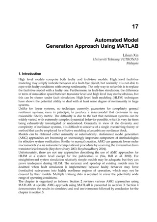


![Engineering Education and Research Using MATLAB412
produced relate to physical quantities, as in the continuous-time domain model, but are less
susceptible to the choice of sampling interval (Wilkinson, Roberts et al. 1991). Initially a
discrete-time system is given in (13):
1 2 1 2( ) ( 1) ( 2) ( ) ( 1) ( 2) ( )na nby t a y t a y t a y t na b u t b u t b u t nb= − − − − − − + − + − + −… … (13)
A linear regression form of the system is shown in (14):
( ) ( )T
y t tϕ θ= (14)
where θ is the parameter vector shown in (15), φ(t) is the regression vector displayed in (16).
[ ]1 2 1 2
T
na nba a a b b bθ = … … (15)
( ) [ ( 1) ( ) ( 1) ( )]T
t y t y t na u t u t nbϕ = − − − − − −… … (16)
The least square estimate (LSE) of the parameter vector can be found from measurements of
u(t) and y(t) using (17) (Ljung 1999):
1
1 1
1 1
( ) ( ) ( ) ( ) ( )
N N
T
t t
t t t t y t
N N
θ ϕ ϕ ϕ
−
= =
⎡ ⎤ ⎡ ⎤
= ⎢ ⎥ ⎢ ⎥
⎣ ⎦ ⎣ ⎦
∑ ∑ (17)
Its recursive form is expressed in (18), where ε(t) is the prediction error, λ(t) represents
forgetting factor (ff), P(t) indicates covariance matrix, and L(t) is the gain vector.
( ) ( 1) ( ) ( )
( ) ( ) ( ) ( 1)
( 1) ( )
( )
( ) ( ) ( 1) ( )
1 ( 1) ( ) ( ) ( 1)
( ) ( 1)
( ) ( ) ( ) ( 1) ( )
T
T
T
T
t t L t t
t y t t t
P t t
L t
t t P t t
P t t t P t
P t P t
t t t P t t
θ θ ε
ε ϕ θ
ϕ
λ ϕ ϕ
ϕ ϕ
λ λ ϕ ϕ
= − +
= − −
−
=
+ −
⎡ ⎤− −
= − −⎢ ⎥
+ −⎢ ⎥⎣ ⎦
(18)
The linear regression is then restructured using the delta operator as shown in (19)
(Middleton and Goodwin 1990), where δ represents delta, q is the forward shift operator
and Ts is the sampling interval. The relationship between δ and q is a simple linear function,
so δ can offer the same flexibility in the modeling of discrete-time systems as q does.
1q
Ts
δ
−
= (19)
This operator behaves as a form of the forward-difference formula, as shown in (20) (Burden
and Faires 1985). This is used extensively in numerical analysis for computing the derivative
of a function at a point.
( ) ( )
'( )
f x h f x
f x
h
+ −
= (20)](https://image.slidesharecdn.com/engineeringeducationandresearchusingmatlab-160628213608/85/Engineering-education-and_research_using_matlab-422-320.jpg)
![Automated Model Generation Approach Using MATLAB 413
The delta operator makes use of the discrete incremental difference (or delta) operator that
whilst operating on discrete data samples, is similar to those of the continuous-time Laplace
operator. A better correspondence can be obtained between continuous and discrete time if
the shift operator is replaced by a difference operator that is more like a derivative
(Middleton and Goodwin 1990).
A similar procedure is used to achieve regression based on the delta operator. This starts by
considering a continuous time transfer function shown in (21).
1 0
0 1
1 0
1
( )
n n
n
m m
m
b s b s b s
G s
s a s a s
−
−
+ +
=
+ +
…
…
(21)
When Ts is sufficiently short, the continuous time transfer function G(s) is equal to the delta
transfer function G(δ) (Middleton and Goodwin 1990) displayed in (22).
1 0
0 1
1 0
1
( )
( )
( )
n n
n
m m
m
y t b b b
G
u t a a
δ δ δ
δ
δ δ δ
−
−
+ +
= =
+ +
…
…
(22)
After arranging this, equation (23) is obtained:
1
1 0( ) ( ) ( ) ( ) ( )m m n
m ny t a a y t b b u tδ δ δ−
= − + + + + +… … (23)
This can be written as (24) (Middleton and Goodwin 1990), which is similar to (14):
( ) ( )m T
y t tδ ϕ θ= (24)
where
[ ]1 2 0 1
T
m na a a b b bθ = … …
1 0
( ) [ ( ) ( )T m
t y t y tϕ δ δ−
= − −… 0
( ) ( )]n
u t u tδ δ…
Using a similar approach to LSE in the discrete-time transform, the parameter vector is
obtained using the delta operator in (25):
1
1 1
1 1
( ) ( ) ( ) ( ) ( )
N N
T m
t t
t t t t y t
N N
θ ϕ ϕ ϕ δ
−
= =
⎡ ⎤ ⎡ ⎤
= ⎢ ⎥ ⎢ ⎥
⎣ ⎦ ⎣ ⎦
∑ ∑ (25)
RLS is also obtained in (26), as shown that it is similar to equation (18), the difference is that
the vectors including , ,yθ ε have been deltarised.
( ) ( 1) ( ) ( )
( ) ( ) ( ) ( 1)
( 1) ( )
( )
( ) ( ) ( 1) ( )
1 ( 1) ( ) ( ) ( 1)
( ) ( 1)
( ) ( ) ( ) ( 1) ( )
m T
T
T
T
t t L t t
t y t t t
P t t
L t
t t P t t
P t t t P t
P t P t
t t t P t t
θ θ ε
ε δ ϕ θ
ϕ
λ ϕ ϕ
ϕ ϕ
λ λ ϕ ϕ
= − +
= − −
−
=
+ −
⎡ ⎤− −
= − −⎢ ⎥
+ −⎢ ⎥⎣ ⎦
(26)](https://image.slidesharecdn.com/engineeringeducationandresearchusingmatlab-160628213608/85/Engineering-education-and_research_using_matlab-423-320.jpg)
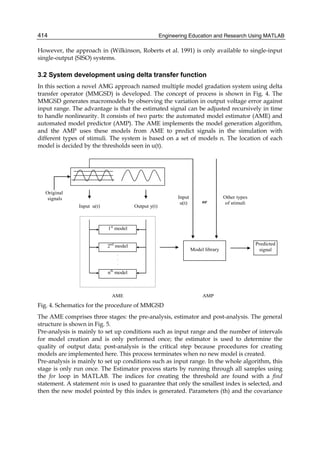
![Automated Model Generation Approach Using MATLAB 415
matrix (p) in each model need to be created and updated. The innovation error (epsi) and
residual error (epsilon) are all calculated. Moreover, the prefilter needs also to be updated.
The estimation is not over until all samples finish (Ljung 1999).
start
Pre-analysis
Create a model
Post-analysis
Estimator
yes
no
end
Is new model
needed?
Fig. 5. The flowchart for the AME
Post-analysis is the critical step because procedures for creating models are run here. The
workflow is described in Fig. 6. The decision to add a new model to an interval of input
voltage is based on (27), where mediumRange is half of the difference between the
maximum amplitude of the error (highInterval) and the minimum amplitude of the error
(lowInterval) for the interval. criticalRange is the equivalent summation. criteria calculated
for the interval results from the comparison of these measures and that of the central
interval of the simulation (mediumRange(central)).
( ) /2
( )/2
[ ( )]
mediumRange highInterval lowInterval
criticalRange highInterval lowInterval
criteria mediumRange mediumRange central criticalRange
= −
= +
= − −
(27)
If the difference between two mediumRange is greater than the criticalRange, one model is
added within the jth interval (if there are j intervals), otherwise no action is taken. If j is
greater than a central point, the threshold will be set at the lower range, otherwise it is set at
the higher range in order to obtain the position close to the central point. In order to increase](https://image.slidesharecdn.com/engineeringeducationandresearchusingmatlab-160628213608/85/Engineering-education-and_research_using_matlab-425-320.jpg)
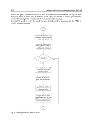


![Automated Model Generation Approach Using MATLAB 419
( ) ( ) ( ) ( )y y 1 y 2 y 3t t t t− − − (34)
The number of iterations depends on a variable called numb, the reason to use the variable is
that during undeltarising, vectors such as output vector need to be undeltarised once to
obtain the value at next time, but during the prefilter update, it needs to be fully
undeltarsied. If a full undeltarisation is required, the variable is set to 0, otherwise an integer
is selected. If the number is greater than the size of the vector array an error message is
produced.
3.2.3 Two functions utility in MMGSD
It is known that the delta operator is a very high gain system because of the sampling
interval Ts (10us in this case), so it is important not to put a vector or a variable in the wrong
place during the manipulation, otherwise, the whole process may numerically explode very
quickly.
In this subsection some key modifications in the MMGSD based on the functions defined
above are described in the following subsections.
3.2.3.1 The AME
In order to obtain the deltarised output data dy at current time and the deltarised vector
array dphi, the vector array phi (φ) and the original output data y at current time are
needed. The deltarise function is employed in (35).
( )( )4y y ,dphi deltarise phi iiia Ts= ⎡ ⎤⎣ ⎦ (35)
where iiia indexes the array for the output vector in phi. Ts is the sampling interval, dphi4y
is the deltarised vector array for output, in which the first element is dy, and all other
elements are assigned to dphi(iiia).
Similarly input vectors u and e, and the noise vector c are deltarised values for dphi.
However, their deltarised values at the current time are not required.
Secondly in the prefilter ztil in RML, the relationship between psi (ψ) and phi (φ) in z
transform is expressed as: phi(t) = c(z)*psi(t), or phi(t) = psi(t)+c1psi(t-1)+…+cncpsi(t-nc),
where c is the polynomial coefficients [1, c1, …, cnc] for noises to improve the property of psi
so that the estimator converges more reliable. It is seen that phi(t) is related to psi at both
current and previous time. The relationship between psi and phi in delta (δ) transform is
expressed as in (36), where the c polynomial is a deltarised version of the coefficients,
( ) ( ) ( )phi t c psi tδ= ⋅ (36)
or its full expression in (37).
1 1 2
1( ) ( ) ( ) ... ( )nc nc nc
ncphi t nc psi t nc c psi t nc c psi t ncδ δ δ− − −
− = − + − + + − (37)
To achieve deltarised psi at current time, this equation is manipulated as shown in (38). It is
a two-dimensional array, the number of rows is equal to the size of vectors in phi and the
number of columns is equal to the number of terms in the c polynomial.
( ) ( ) ( ) ( )1 1 2
1
nc nc nc
ncpsi t nc phi t nc c psi t nc c psi t ncδ δ δ− − −
− = − − − −…− − (38)](https://image.slidesharecdn.com/engineeringeducationandresearchusingmatlab-160628213608/85/Engineering-education-and_research_using_matlab-429-320.jpg)
![Engineering Education and Research Using MATLAB420
When using the z transform, (Ljung 1999) makes use of the fact that past values of psi and
phi are readily available in the estimator, so that psi(t) can be obtained easily from available
data vectors in the estimator. This is because the nature of the data does not change with
storage position in the data vector. However, when using the delta transform ( )-1
-nc
psi t ncδ
cannot be obtained using the same procedure, because samples in the data vector are
different orders of δ. All these data vectors have to be refilled at each sampling interval.
The vectors in ( )1nc
psi t ncδ −
− are shown in (39), if, for example, the coefficients array nn is
[3 4 2 1 4].
2 0 3 0 1 0 3 0
( 3) ( 3), ( 4) ( 4), ( 2) ( 2),1, ( 4) ( 4)y t y t u t u t t t v t v tδ δ δ δ δ ε δ ε δ δ− − − − − − − − − −… … … (39)
2 0
( 3) ( 3)y t y tδ δ− − − −… are obtained by deltarising ( 1) ( 3)y t y t− − − −… using deltarise
function. The undeltarise function in 0 is also required to firstly fully undeltarise each row
of dpsi at previous time to achieve the current time psi(t), e.g., ( 1) ( 3)y t y t− − − −… is
achieved by fully undeltarising 2 0
( 3) ( 3)y t y tδ δ− − − −… . The undeltarise function is
employed again but only for a single iteration (numb = 1) to obtain dpsi the next time, so
this matrix is shifted forward once. The last term (δ0psi) in the array is then thrown away,
so δ1psi becomes δ0psi and so on in order to add the new array in front and keep the
algorithm consistent.
Finally the vector array phi is updated with the new estimation including the noise vector
that is updated by residual error epsilon. We must keep in mind that depsilon is the
deltarised version of epsilon, in this case we only have depsilon at current time, thus the
undeltarise function is needed for epsilon, as shown in (40).
epsilon = undeltarise([depsilon dphi(iiic)], Ts, 0) (40)
where dphi(iiic) includes noise vectors at previous time, iiic is the index array for noise
vectors in dphi, Ts is the sampling rate, 0 indicates the full undeltarisation as has been
discussed above.
3.2.3.1 The AMP
Similar to the AME both the deltarise and undeltarise functions are required through the
system. Unlike the AME, the predicted value y is used for updating the vector array phi,
whereas in the AME inputs u, e and output y are obtained from the training data.
To obtain the output data y, dy is fully undeltarised by employing the undeltarise function
shown in (41):
y = undeltarise([dy -dphi(iiia)], Ts, 0) (41)
where dphi(iiia) includes the previous deltarised output vector, iiia is the array for the
outputs in dphi, Ts is the sampling rate, 0 indicates the full undeltarisation is utilized.
4. Results and discussions
In this subsection the MMGSD is evaluated based on two experiments. The data obtained
from a two-stage CMOS operational amplifier (op amp) as shown in Fig. 7. The op amp is
used in an open-loop configuration.](https://image.slidesharecdn.com/engineeringeducationandresearchusingmatlab-160628213608/85/Engineering-education-and_research_using_matlab-430-320.jpg)


![A Matlab Genetic Programming Approach to Topographic Mesh Surface Generation 429
y, which was approximated to a third order Taylor series (Arfken, 1980). Coefficients were
adjusted by a Least Square Algorithm. Obtained results were, in general, acceptable.
However, there were a significant number of points where the proposed method did not
provide appropriate estimation (Mendoza et al., 1996). These points corresponded to regions
of peaks and valleys surrounded by very different topographic points.
In order to improve the quality of the approximation, Mendoza (2002) proposed the use of
algorithms belonging to the EAs field. As it is known, EAs are optimization techniques
based on the concepts of natural selection and evolution. This work is then focused on the
use of one of these evolutionary techniques, Genetic Programming (Banzhaf, et al., 1998).
In the present work, representing a topographic surface by means of a mathematical
function is proposed and the problem is formulated as a symbolic regression using
traditional genetic programming. A GP Toolbox for MATLAB is then developed and
detailed in next sections.
3. Genetic programming
Nature has provided the inspiration for the design of computational algorithms in a variety
of ways. These computational processes have taken two main natural systems as their basis
that is the brain and the genetic evolution theory. EAs are one of these computational models
and are proposed in this work for modelling topographic surface.
EAs, also known as Evolutionary Computation (EC), use computational models of
evolutionary processes in the design and implementation of computer-based problem
solving. A general definition and classification of these evolutionary techniques is given in
Bäck (1996). He defines an EA as a search and optimisation algorithm, inspired by the
process of natural evolution, which maintains a population of structures that evolve
according to rules of selection and other operators such as recombination and mutation.
Here, the structure of all evolution-based algorithms is shown in Figure 1.
The adaptive search algorithm called Genetic Programming (GP) was designed by Koza
(1990). GP is an evolution-based search model that is a subclass of the popular GAs
[Holland, 1975; Goldberg, 1989]. Koza introduced a more complex representation based on
computer programs. Although finding algorithms or programs is more difficult than finding a
single solution, it is more useful since generalised solutions work for an entire class of tasks.
PROGRAM Evolution-Based Algorithm
t = 0
Create Initial Population P(t)
Evaluate Initial Population P(t)
While (not termination_criterion) do
t = t + 1
Select Individuals for Reproduction P(t) from P(t-1)
Alter P(t)
Evaluate New Population P(t)
end
Fig. 1. Evolution-based algorithm](https://image.slidesharecdn.com/engineeringeducationandresearchusingmatlab-160628213608/85/Engineering-education-and_research_using_matlab-439-320.jpg)


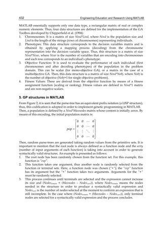

![Engineering Education and Research Using MATLAB434
5 1 3 1004 6 1001 4 7 1001 6 1002 0
1 6 1001 3 1002 1003 0 0 0 0 0 0
4 3 1001 1002 1 1001 1002 0 0 0 0 0
pop
⎡ ⎤
⎢ ⎥
⎢ ⎥=
⎢ ⎥
⎢ ⎥
⎣ ⎦
Genetic operators are applied on these prefix representations by selecting a random
crossover node in the first parent in the interval [1, MaxNodesPopi] and a random node in the
second parent between [1, MaxNodesPopi+1], where MaxNodesPop is a Nind column vector
containing information related to the number of nodes of each individual into the
population. This vector is updated each time crossover or mutation is performed. After that,
associate expression to these selected nodes are taken and exchanged creating two new
individuals.
In the case of mutation, again a node is randomly selected in the range [1, MaxNodesPopi]
and the syntactically valid associate sub-expression is eliminated and a new sub-expression
is inserted. This is created from the primitive sets and using the routine of creating initial
population.
If a new individual generated by means of crossover or mutation exceeds the allowed
maximum size (maximum number of nodes), a new randomly selected node is taken in the
range defined by the position of the previously selected node and MaxNodePopi. This fact
avoids that individuals grow rapidly causing bloat1.
An example of crossover on the MATLAB GP representation is exemplified in Figure 4.
Previous pop matrix is considered in this example. It is important to mention that the
individual selection mechanism can be any method (roulette wheel, tournament, stochastic
universal selection) and it is borrowed from the GA Toolbox, as well as the fitness
assignment mechanism.
5.1 Function evaluation
In order to evaluate each individual into the population, a bottom-up parser must be
constructed as a MATLAB function. Based on primitive set defined in Table 1 and the last
individual of pop matrix from Figure 3, this program is evaluate as illustrated in Figure 5
considering that the variables X and Y take the following values [-3, -2, -1, 0, 1, 2, 3]T and [0,
1, 2, 3, 4, 5, 6]T, respectively. The output of the evaluated individual (information at the root
node) is a vector of size Nx1, where N is the number of data points, in this simple example N
is equal 7. Thus, the objective function is defined as the minimization of the estimated mean
quadratic error produced between the output of each program (individual) and the real
values of the topographic elevation. This is expressed in the following equation:
∑ −=
=
N
1j
2
ijji 'zz
N
1
f
where fi is the objective value of the i-th individual, z is the vector of measured topographic
elevations, z’ is the vector of estimated topographic elevations for N recorded coordinates.
The objective value is scalar and the fitness assignment mechanism described in
Chipperfield et al. (1994) can be straightforward applied. Observe that for the GP Toolbox
1 Bloat is the rapid growth of programs produced by genetic programming.](https://image.slidesharecdn.com/engineeringeducationandresearchusingmatlab-160628213608/85/Engineering-education-and_research_using_matlab-444-320.jpg)

![Engineering Education and Research Using MATLAB436
Fig. 5. A bottom-up parser to evaluate GP individuals
6. Estimation of topographic surface by means of GP toolbox in MATLAB
In this section, the MATLAB GP toolbox is applied to model and estimate the topographic
elevation of the region shown in Figure 6. The number of available topographic data was
1600 points corresponding to the Mezcalapa river zone located at the southeast of the
Mexican Republic. In order to apply the evolutionary methods, the following considerations
were taken into account:
a. The function set was composed of the four basic arithmetic operators, trigonometric
functions (sine and cosine) and the square root sqrt function. Thus, the arity set was
defined as {2, 2, 2, 2, 1, 1, 1}, the arithmetic functions take two input arguments and the
remaining functions take one input argument.
b. The terminal set consisted of the independent variables (coordinates) x and y, and the
ephemeral random constants in the range [-1, 1].
c. The termination criterion was set as the maximum number of generations.
d. In order to evaluate the performance of each individual into the population, estimate
mean squared error between the topographic elevation obtained by the individual and
the known elevation z was used.
e. The selection mechanism used in these experiments was tournament selection with
tournament of size 3.
f. The population was composed of 100 individuals of a maximum size of 256 nodes.
g. Probabilities of crossover and mutation were set to 0.95 and 0.05, respectively.
h. Finally, ten independent runs were carried out for each sub-region.](https://image.slidesharecdn.com/engineeringeducationandresearchusingmatlab-160628213608/85/Engineering-education-and_research_using_matlab-446-320.jpg)

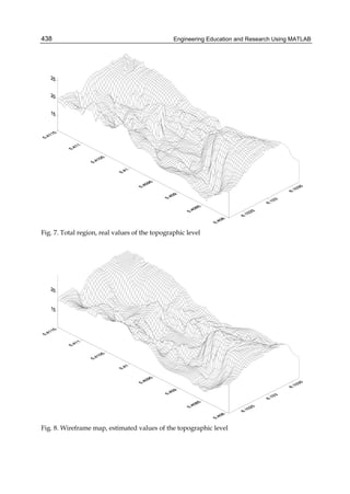


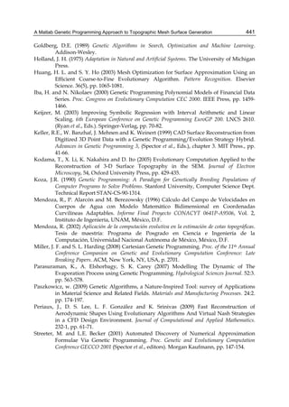


![Engineering Education and Research Using MATLAB444
letter to L’Hospital over three hundred years ago and the earliest more or less systematic
studies have been made in the beginning and middle of the 19th century by Liouville,
Riemann and Holmgren. In the literature, people often use the term “fractional order (FO)
calculus”, or “fractional order dynamic system” where “fractional” actually means “non-
integer” (Oldham, 1974; Petras, 2006; Podlubny, 1999; Tavazoei et al., 2008; Zhao & Xue,
2008).
The definitions most commonly used in the literature are the Riemann-Liouville definition,
the Grünwald-Letnikov definition, and the Caputo definition, as given below:
a
tn
α
a t n 1 (n α)
1 d f( τ )
D [f(t)] dτ
Γ(n α) dt (t τ) − −
⎞⎛
= ⎟⎜ ∫⎜ ⎟− −⎝ ⎠
(1)
[ ]
at
h
α
a t αh 0 k 0
1 Γ(α k)
D f(t) lim f(t kh)
Γ(k 1)Γ(α)h
⎡ ⎤−
⎢ ⎥
→ =
+
= −∑
+
(2)
(n)t
α
a t α n 1
a
1 f (τ )
D [f(t)] dτ
Γ(α n) (t τ) − +
= ∫
− −
(3)
for n-1 < α < n and where Γ(·) is the Gamma function, and z⎡ ⎤⎢ ⎥ means the integer part of z.
The “memory” effect of these operators is demonstrated by (1) and (2), where the
convolution integral in (1) and the infinite series in (2) reveal the unlimited memory of these
operators, ideal for modeling hereditary and memory properties in physical systems and
materials. The initial conditions for the fractional order differential equations with the
Caputo derivative (3) are of the same form as the initial conditions for the integer-order
differential equations (Baleanu et al., 2010; Kilbas et al., 2006; Tavazoei & Haeri, 2008).
Two general properties of the fractional-order derivative are of major interest here. The first
is the composition of fractional with integer-order derivative and the second is the property
of linearity. Similar to integer-order differentiation, fractional-order differentiation fulfils the
relations
α kn
β α β β kα
a t a t a t a t t a
k 0
(t a)
D ( D f(t)) D f(t) [ D ]
Γ(1 α k)
− −
+ −
=
=
−
= − ∑
− −
(4)
α α α
a t a t a tD [η f(t) λg(t)] η[ D f(t)] λ[ D g(t)]++ = (5)
In addition, fractional order systems may have other features that make them more suitable
for the study of electronic circuits when most of the desired specifications are not readily
achieved by traditional models (Petras, 2006; Trzaska, 2009).
2.2 Fractional order differential equations
A fractional order linear time invariant system can be represented in the form of a scalar
differential equation of fractional order as follows:
αα α α β β0n n 1 n 2 m m 1
n n 1 n 2 0 m m 1
ββ 0m 1
m 2 0
a D y(t) a D y(t) a D y(t) a D y(t) b D u(t) b D u(t)
b D u(t) b D
− − −
− − −
−
−
+ + + + = +
+ + + u(t)
(6)](https://image.slidesharecdn.com/engineeringeducationandresearchusingmatlab-160628213608/85/Engineering-education-and_research_using_matlab-454-320.jpg)


![Matlab Solutions of Chaotic Fractional Order Circuits 447
where Af =Cf Lf , Bf = GLf denote constant coefficients and iz(t) is a time varying right hand
side term.
(a) (b)
Fig. 1. Linear circuit containing fractors Lf and Cf: a) structure, b) input and output signals
2
1.5
1
0.5
0
-0.5
H(t),u(t)
H(t)
u(t)
time [s]
0 1 2 3 4 5 6 7 8 9 10
(a) (b)
Fig. 2. Voltage source connected to uniform RC line: a) scheme of the circuit, b) impulse H(t)
and unit-step u(t) responses
To determine the solution of (12) we have used a special numerical procedure based on the
Bagley-Torvik scheme (Trzaska, 2010). Taking into account Af = 1.25s2, Bf = 0.5s3/2 and
iz(t) = 8A for 0 < t < 1s with iz(t) = 0 for t >1s and applying the mentioned numerical
procedure implemented in MATLAB (Attia, 1999; Redfern & Campbell, 1998) we obtain the
solution shown in Fig. 1b. It is easily seen that the circuit displays comprehensive dynamical
behavior, such that the transient output signal varies very slowly in respect to the excitation.](https://image.slidesharecdn.com/engineeringeducationandresearchusingmatlab-160628213608/85/Engineering-education-and_research_using_matlab-457-320.jpg)
![Engineering Education and Research Using MATLAB448
Next, let us consider a fractional order circuit shown in Fig. 2a. It represents the connection
of a voltage source e(t) exhibiting internal conventional inductance L=1H with a very long
(l ≈ ∞) uniform RC transmission line. The transmission line can be represented by a circuit
with uniformly distributed constant parameters and the whole circuit considered at the
line’s input is described by the following fractional order model
3/2
3/2
C d u(t)
L u(t) e(t)
R dt
+ = (13)
where u(t) denotes the voltage at the line’s input.
However, in order to effectively analyze such systems, it is necessary to develop
approximations to the fractional operators using the standard integer order operators. In the
work that follows, the approximations are effected in the Laplace variable s = α + jω. It
should be pointed out that the resulting approximations provide sufficient accuracy for the
time domain hardware implementations (Faleiros et al., 2006).
For the sake of simplicity of notations without any loss of generality we assume in what
follows that 3 21
L CR 1s−
= and zero initial conditions are taken into consideration. Thus,
applying Kirchhoff laws and relations describing circuit elements in the Laplace transform
domain leads to the following fractional order model
3/2
1
U(s) E(s)
s 1
=
+
(14)
where U(s) and E(s) denote the Laplace transforms of u(t) and e(t), respectively. Now taking
into account the inverse Laplace transforms of both sides of (14) yields
t
-1
3/2
0
u(t) [U(s)] H ( 1,τ)e(t τ)dτ= = − −∫L (15)
where the function H3/2(-1,t) is determined by
3n/2
3/2 3
n 0 2
t
H ( 1,t) t
Γ( (n 1))
∞
=
− = ∑
+
(16)
and represents the impulse response of the circuit. In the case of the source voltage
e(t) = E0η(t) with E0 = const and η(t) denoting Heaviside function the voltage at the line’s
input is determined as follows
3/2
η 3/2 0u (t) [η (t) E (t )]E= − (17)
where E3/2(t) denotes the Mittag-Leffler function for a = 3/2 and b = 1. Taking into account
(16) and (17) we can plot the circuit response for the inputs in the form of Dirac impulse and
unit-step functions (E0 = 1) separately. The computed responses are presented in Fig. 2b. It
has to be noted that in almost all cases the impulse responses of fractional order circuits are
related to the Mittag-Leffler function (Podlubny, 1999), which is effectively the fractional
order analog of the exponential function. With this knowledge, it has been possible to better
clarify the time responses associated with fractional order circuits.](https://image.slidesharecdn.com/engineeringeducationandresearchusingmatlab-160628213608/85/Engineering-education-and_research_using_matlab-458-320.jpg)
![Matlab Solutions of Chaotic Fractional Order Circuits 449
Interestingly, an alternative approach to the solution of the above circuit can be sought by
applying Symbolic Math Toolbox. On the base of (14) we can determine the fractance
(fractional transfer function) of the circuit, namely
3/2
1
(s)
s 1
=
+
F (18)
Considering s1/2 as basic complex variable we can expand right hand side of (18) in the
following partial fractions
jπ /3 jπ /3
1/2 jπ /3 jπ /31/2 1/2
1 1 e e
(s) ( )
3 s 1 s e s e
−
−
= − −
+ − −
F (19)
Observe, that first term in (19) with pole at -1 on the complex plane with variable s1/2
introduces an important damping of the impulse response and the remaining terms with
poles at e±j2π/3 are responsible on the damping oscillations and all terms taken in the whole
give the circuit response which oscillates at an over damped rate. This is easily seen from
the time-variations of H(t) presented in Fig. 2b. The diagram corresponds to the expression
j2π /3 j2π /3
j2π /3 j(4π /3)t j2π /-1 t
3/2
j2π /3 j(4π /3) j2π /3
1 1 e e3F(s) H ( 1,t) [ e e e erfc(e t)
3 πt πt πt
te e erfc(e t)]
−
− − −
= − = − − + −
+
L
(20)
which has been determined by applying the inverse Laplace commands from the Symbolic
Math Toolbox. It is worth noting that the form of (20) is an alternative form of (16).
Now, to highlight numerous benefits from the application of suitable procedures contained
in the MATLAB package we consider the circuit shown in Fig. 3a. It is composed of a real
coil Lf and a supercapacitor Cf, both elements considered as fractors and a zero order voltage
Lf
Cf
+ -
Au(t)
u(t)
i(t)
R
uL
uR
0 0.1 0.2 0.3 0.4 0.5 0.6 0.7 0.8 0.9 1
0.05
0.1
0.15
0.2
0.25
0.3
0.35
0.4
0.45
0.5
R=0.25
0.5
1.0
2.0
time [s]
u(t)[V]u(t)[V]
R=0.25
0.5
1.0
2.0
Fig. 3. Fractional order circuit with controlled source and resistor: a) circuit scheme,
b) capacitor’s voltage for various resistances
source controlled by the supercapacitor’s voltage vC (t) = Au(t). Applying circuit laws we
obtain the following set of expression in terms of fractional order derivatives](https://image.slidesharecdn.com/engineeringeducationandresearchusingmatlab-160628213608/85/Engineering-education-and_research_using_matlab-459-320.jpg)
![Engineering Education and Research Using MATLAB450
1 2
1 2
α α
f L f R Cα α
d i(t) d u(t)
L u (t), C i(t), Ri(t) u (t), Au(t) v (t)
dt dt
= = = = (21)
with the same symbol meanings as in Fig. 3a. Applying the voltage Kirchhoff law and
taking into account (21) and rearranging the terms we obtain the following fractional order
equation
1 2 2
1 2 2
α α α
f f fα α α
d i(t) d u(t)
L C RC u(t) Au(t)
dt dt
+
+
+ + = (22)
If we assume that Lf Cf ≡ 1, A =3, R =var, and Cf =const then equation (22) takes the form
1 2 2
1 2 2
α α α
α α α
d u(t) d u(t)
R 2u(t) 0τ
dt dt
+
+
+ − = (23)
where Rτ = RCf denotes the time constant of the R, Cf series connection. In order to analyze
effectively the above equation it is convenient to apply the standard procedures supplied by
the MATLAB programs package and particularly those from the Symbolic Math Toolbox. In
this regard, the Laplace transform of the initialized fractional-order differential equation (23)
with α1= α2 = ½ takes the form
-1/2
τ -1/2
d
sU(s) u(0) sR U(s) u(0) 2U(s) 0
dt
− + − − = (24)
where U(s)=L [u(t)] denotes the Laplace transform of the capacitor voltage u(t). Solving (24)
with respect to U(s) yields
τ
B
U(s)
s R s 2
=
+ −
(25)
where B=u(0) + d-1/2/dt-1/2 u(0) is a constant depending on circuit initial conditions. Because
(25) contains the fundamental ‘fractional’ poles it can be rewritten, using partial fractions, in
a more simple form as follows
2 1 1 2
B 1 1
U(s) ( )
p p s p ) s p
= −
− − −
(26)
where 2
1
1p ( a a 8)
2
= − + + and 2
2
1p ( a a 8)
2
= − − + denote the fractional poles of U(s) with
a = Rτ. The above result indicates that the response of the initialized fractional order circuit
can be determined by inverse transforming of each term of (26) separately. To accomplish
these tasks, it is convenient rewrite (26) in an equivalent form as follows
1 2U(s) U (s) U (s)= + (27)
with
1 2 1 1 2 2 1 2U (s) B /((p p )( s p )), U (s) B /((p p )( s p ))= − − = − − − (28)](https://image.slidesharecdn.com/engineeringeducationandresearchusingmatlab-160628213608/85/Engineering-education-and_research_using_matlab-460-320.jpg)


![Matlab Solutions of Chaotic Fractional Order Circuits 453
parameters of the circuits bifurcate have been performed and the one showed is typical for
MMOs. The importance of MMOs lies mainly in the fact that during bifurcations the circuits’
dynamics undergoes complex transitions between various stable and chaotic modes,
including the mixed mode oscillations, period doubling bifurcations and chaotic responses.
In most cases the solutions pertain to canard phenomenon. The most accepted and popular
approach to explain the MMOs phenomenon in R3 is that they result from a combination of
canard solutions around a fold singularity and relaxation spikes coupled together by a
special global return mechanism (Trzaska & Marszalek, 2011).
(a) (b)
Fig. 4. Modified Chua’s circuit: a) scheme with fractors C1, L, C3 and I = (1 + b)x2,
In = αx12 +βx13, a = const > 0, b = const > 0, α < 0 and β > 0, b) MMOs in an integer order case
Using the same element parameters values as the ones assumed above and changing only
the form of the nonlinear characteristic to 0.88 ≤ α ≤ 1 with step size 0.0005 we obtain the
solutions exhibiting bifurcations between MMOs and chaotic oscillations. In this chapter, we
use two no-chaos criteria for a fractional order circuit represented by state variable equation
dqx(t)/dtq = f (x(t)). Those criteria are: (i) x(t) approaches a fixed point; (ii) x(t) is bounded. It
is clear that if a circuit contravenes both of the above conditions, it has necessary, albeit not
sufficient, condition to demonstrate chaotic behavior (Marszalek & Trzaska, 2010).
The code presented below computes bifurcation diagram shown in Fig. 5a. The same code
can be used to compute diagrams for other parameters provided that appropriate changes
are made in the lines with parameters in bold-face.
Main code:
Clear
M = [1 0 0
0 1 0
0 0 1];
x0=[-0.5; 0.2; 0.5];
options = odeset('Mass',M,'RelTol',1e-12,'AbsTol',[1e-14 1e-14 1e-14], 'Vectorized','on');](https://image.slidesharecdn.com/engineeringeducationandresearchusingmatlab-160628213608/85/Engineering-education-and_research_using_matlab-463-320.jpg)
![Engineering Education and Research Using MATLAB454
global t x y z dt alpha
dt=0.01;
for alpha=0.8800:0.0005:1.6000
alpha
clear n
clear m
[t,x]=ode15s(@equations,0:dt:500,x0);
n=length(x(:,1));
m=floor(n/2);
y=diff(x(m,n,1))/dt;
z=diff(y)/dt;
k=1;
clear aa
for i=m:n
t0=t(i); %Comp. local max. pts for m<t<n
option=optimset(’display’,’off’);
zer=fsolve(@differ,t0,option);
if interp1(t(m:n-2),z,zer)>0
aa(k)=interp1(t(m:n),x(m:n,1),zer);
k=k+1;
end
end
kmax=k-1;
h=plot(alpha.*ones(1,kmax),aa,’r.’);
hold on
set(h,’MarkerSize’,0.1);
end
Function equations.m:
function xdot=equations(t,x)
global alpha
a=0.0005; b=0.01; eps=0.01; beta=-1; R=0.3;
xdot(1) = (-x(2) + alpha*x(1)ˆ2 + beta*x(1)ˆ3)/eps;
xdot(2) = x(1) - x(3) - R*x(2);
xdot(3) = a - b*x(2);
xdot = xdot’;
end
Function differ.m:
function f=differ(a)
global t x dt
s=diff(x(m:n,1))/dt;
f=interp1(t(m:n-1),s,aa);
end
Fig. 5 shows the solutions obtained with local maximum values of x1(t) as a function of α. In
all the integrations the initial conditions were zero for all three variables in (31). Note that
the number of local maximum points at the level 0.2 − 0.3 (on the lower fold of the surface
x2 = αx21 + βx31) increases if α increases. The number of upper local maximum points (at the](https://image.slidesharecdn.com/engineeringeducationandresearchusingmatlab-160628213608/85/Engineering-education-and_research_using_matlab-464-320.jpg)


![Matlab Solutions of Chaotic Fractional Order Circuits 457
To compute discrete state variable (36) and to plot their diagrams the code presented below
can be used. The same code can be used for other parameters provided that appropriate
changes are made in the lines with parameters in bold-face (Petras, 2010)
Main code:
Clc
clear
% Numerical Solution of the Fractional-Order Modified Chua's Circuit
% with cubic nonlinearity defined in function fm()
function [h, xdisc]=MOChua(parameters, orders, tfin, x0)
%
% time step
h=0.001; tfin=200;
% number of discrete points
n=round(tfin/h);
%orders of derivatives
q1=0.9; q2=0.9; q3=0.9;
%parameters
alpha=100.0; beta=1.0;gamma=1.0;R=0.1;a=0.0005; b=0.001;a0=1.5; a1=-1;
%initial conditions
x0=0;y0=0;z0=0;
% binomial coefficients
bp1=1; bp2=1; bp3=1;
for j=1:n
b1(j)=(1-(1+q1)/j)*bp1;
b2(j)=(1-(1+q2)/j)*bp2;
b3(j)=(1-(1+q3)/j)*bp3;
bp1=b1(j); bp2=b2(j); bp3=b3(j);
end
% initial conditions setting
x(1)=x0; y(1)=y0; z(1)=z0;
% discretized solution
for i=2:n
x(i)=(alpha*(-y(i-1)+f1(a0,a1,x(i-1))))*h^q1 - back(x, b1, i);
y(i)=(beta*(x(i)-R*y(i-1)-z(i-1)))*h^q2 - back(y, b2, i);
z(i)=(gamma*(a-b*y(i)))*h^q3 - back(z, b3, i);
f(i)=f1(a0,a1,x(i));
end
%plots
t=h:h:tfin;
plot(t,x),grid,pause
plot(x,y),grid,pause
plot(t,x,t,y,t,z),grid,pause
plot3(x,y,z),grid,pause
plot(x,f),grid
%
The codes f1(a0,a1,x) for the characteristic of a nonlinear resistor and back(x,b,i) are as follows](https://image.slidesharecdn.com/engineeringeducationandresearchusingmatlab-160628213608/85/Engineering-education-and_research_using_matlab-467-320.jpg)
![Engineering Education and Research Using MATLAB458
function [fn]=f1(a0, a1, un);
a0=1.5;a1=-1.;
fn=a0*un.^2 + a1*un.^3;
%
function [vo] =back(r, b, k)
%
temp = 0;
for j=1:k-1
temp = temp + b(j)*r(k-j);
end
vo = temp;
%
Simulations were then performed using various qk, k =1, 2, 3, from the value interval 0.8 ÷ 1.1.
In all cases the Lyapunov exponents were computed and one of them at least exhibited
positive value which indicates that the circuit is behaving chaotically. Moreover, the
numerical simulations also indicated that the lower limit of the fractional derivative q of all
state vector components leading to generating chaos takes values from the interval (0.8 ÷0.9).
Therefore, using q = 0.9 as fractional state vector derivative yields the lowest value at 2.7 for
circuit order generating chaos in the modified Chua circuit. The simulation results obtained
for these circuits are presented in Fig. 6 for alpha =100.0, beta = gamma = 1.0, a = 0.0005,
b = 0.005, a0 = 1.5, a1 = -1.
3.2.3 Fractional-order Chua’s circuit with piecewise-linear resistor
Let us explore now the fractional-order modified Chua’s circuit of Fig. 4a but with the
nonlinear resistor exhibiting piecewise-linear current-voltage characteristic. In order to
appreciate the richness of the dynamics of the present variant circuit we involve the
resistor’s piecewise-linear characteristic composed of three linear segments leading to the
form quite similar to that shown in Fig. 6d. It can be described by the formula
n 1 1 2 1I abs(u ) H (u u )= + ⋅ − (39)
where u1 and u2 determine successive segments of the piecewise-linear characteristic
depending on the voltage at the nonlinear resistor terminals. These segments can be
represented as follows
1 1 1 2 2 1 0u a x , u a x a= = + , (40)
where constant coefficients a1 and a2 determine the slopes of particular characteristic
segments, and a0 is the free term. To get a continuous piecewise-linear characteristic the
segments are exactly matched as a result of the concatenation given by the shifted Heaviside
function
1 c
1
1 c
abs(x x )1
H (1 )
2 x x
−
= +
−
(41)
with xc fixed at the point of coordinate x1 corresponding to characteristic folding of
neighboring segments.](https://image.slidesharecdn.com/engineeringeducationandresearchusingmatlab-160628213608/85/Engineering-education-and_research_using_matlab-468-320.jpg)
![Matlab Solutions of Chaotic Fractional Order Circuits 459
0 10 20 30 40 50 60 70 80 90 100
-0.4
-0.2
0
0.2
0.4
0.6
0.8
1
1.2
Time [s]
0 10 20 30 40 50 60 70 80 90 100
-0.4
-0.2
0
0.2
0.4
0.6
0.8
1
1.2
Time [s]
(a) (b)
-0.4 -0.2 0 0.2 0.4 0.6 0.8 1 1.2
-0.05
0
0.05
0.1
0.15
0.2
-0.5 0 0.5 1 1.5
0
0.05
0.1
0.15
0.2
0.25
0.3
0.35
0.4
0.45
0.5
x1
f1(x1)
x1
x2
(c) (d)
Fig. 6. Simulation results for a modified Chua’s circuit of fractional orders q1 = q2 = q3 = 0.9:
a) state variable x1(t), b) all state variables: x1(t) - in blue, x2(t) - in green, x3(t) – in red,
c) x2(t) versus x1(t), d) nonlinear resistor’s characteristic f1(x1)= 2 3
1 11.5x x−
To perform simulations of the fractional-order modified Chua’s circuit with nonlinear
resistor characteristic determined by (39) we can use the above presented MATLAB code
after changing only the code corresponding to the nonlinear term by the following one
function [fn]=f2(a0, a1, a2, u0, un);
a0=1.0; a1=1.5; a2=-0.75; u0=1.0;
J1=abs(un-u0)./(un-u0);H1=0.5*(1+J1);
u1=a1*un;u2=a2*un+a0;
fn=abs(u1)+H1.*(u2-u1);
where appropriate changes can be made in parameters in bold-face, similarly to the main code.
The resulting characteristic for a range of parameters assumed as above are shown in Fig. 7a.
A slight modification of arguments of the code above enables to generate other forms of
piecewise-linear characteristics of the nonlinear resistor. For instance, the case of 5-segment
characteristic obtained by such modified code is presented in Fig. 7b.
It is worth noticing that the piecewise-linear models are an attractive alternative to
continuous nonlinear ones because they are both efficient in memory use and economical in
computation time, despite the fact that the derivation of a model usually requires two steps:](https://image.slidesharecdn.com/engineeringeducationandresearchusingmatlab-160628213608/85/Engineering-education-and_research_using_matlab-469-320.jpg)
![Engineering Education and Research Using MATLAB460
first, the piecewise-linear approximation of nonlinear elements’ characteristics, and second,
their algebraic representations. Applying such an approach to studies of nonlinear circuits
leads to piecewise-linear differential equations yielding a pervasively better understanding
of various problems in applications. For instance, the piecewise-linear models for operational
amplifiers (op amps) and operational transconductance amplifiers (OTA’s) are both simple
and frequently used. Another way of approximating dynamic circuits with semiconductor
diodes can be obtained by replacing the real characteristic by piecewise-linear functions
between diode current and voltage.
-2 -1.5 -1 -0.5 0 0.5 1 1.5
-0.1
0
0.1
0.2
0.3
0.4
0.5
0.6
-0.5 0 0.5 1 1.5 2
-0.6
-0.4
-0.2
0
0.2
0.4
0.6
0.8
1
1.2
1.4
unx1
f2(x1)
f3(x1)
x1
(a) (b)
Fig. 7. Piecewise-linear characteristics of the nonlinear resistor: a) 3- segments, b) 5-segments
As it is well known nonlinear devices are already present in a great variety of applications
in both power-electronic engineering and signal processing, and in many electrical networks
controlling elements like thyristors. To reduce the simulation time of the transient behavior
of such circuits and for analysis purposes (e.g., stability or chaos (Tang & Wang, 2005;
Trzaska, 2007)), these circuit components are often modeled using piecewise-linear
characteristics. Piecewise-linear circuits exhibit most of the phenomena of fractional order
nonlinear circuits being yet weakly penetrating. Computer simulations of the suggested
discrete maps with memory prove that the nonlinear dynamical circuits, which are
described by the equations with fractional derivatives, exhibit a new type of chaotic
behavior. This type of behavior demonstrates a fractional generalization of attractors. The
subsequent numerical simulation results demonstrate this claim.
3.2.4 Chaotic oscillations in the circuit with piecewise-linear resistor
For the modified Chua’s circuit of different fractional orders q = [q1, q2, q3]’ we have chosen
function f(x) and the circuit parameters R, L, C1, C3, a, b, and h to satisfy the conditions of
numerical stability, convergence and accuracy, so that the model (36) with appropriately
adapted piecewise-linear characteristic (code for f2(a0, a1, a2, u0, un)) generates regular
oscillations or demonstrates chaotic behaviors. For one of the chaotic circuits given in Fig. 4a
with alpha = 1.5, beta = 0.85, gamma=1.0, R=0.0, a=0.005, b= 0.05, and piecewise-linear
characteristic shown in Fig. 7a we have numerically investigated the sensitivity of the circuit
states to the fractional orders q1, q2 and q3. In all computations performed we have fixed
initial conditions to be zero. The obtained numerical simulations demonstrated that the non-
regular oscillations specified by chaotic attractors can be generated for the components of](https://image.slidesharecdn.com/engineeringeducationandresearchusingmatlab-160628213608/85/Engineering-education-and_research_using_matlab-470-320.jpg)
![Matlab Solutions of Chaotic Fractional Order Circuits 461
the vector fractional derivative q taking values from the set (0.8 ÷1.0). The chaotic dynamics
was identified in two fractional order modified Chua’s circuits with 3-segments and 5-
segments piecewise-linearity.
-0.5 -0.4 -0.3 -0.2 -0.1 0 0.1 0.2 0.3 0.4 0.5
-0.1
0
0.1
0.2
0.3
0.4
0.5
0.6
0.7
x1(t)]
x2(t)
0 500 1000 1500
-0.5
-0.4
-0.3
-0.2
-0.1
0
0.1
0.2
0.3
0.4
0.5
time[s]
Statevariablex1(t)
(a) (b)
-0.5
-0.4
-0.3
-0.2
-0.1
0
0.1
0.2
0.3
0.4
0.5
-0.1
0
0.1
0.2
0.3
0.4
0.5
0.6
0.7
-0.04
-0.03
-0.02
-0.01
0
0.01
0.02
0.03
0.04
x1(t)
x2(t)
x3(t)
-0.05 -0.04 -0.03 -0.02 -0.01 0 0.01 0.02 0.03 0.04 0.05
-0.1
0
0.1
0.2
0.3
0.4
0.5
0.6
0.7
x3
x2
(c) (d)
Fig. 8. Results of simulations for modified Chua circuits with three segments of piecewise-
linear characteristic: a) state variable x1(t), b) phase trajectory x2(t) versus x1(t), c) 3D phase
trajectory, d) phase trajectory x2(t) versus x3(t)
-2.5 -2 -1.5 -1 -0.5 0 0.5 1 1.5
-0.1
0
0.1
0.2
0.3
0.4
0.5
0.6
x1]
x2
x1(t)
x1(t)
-0.1
0
0.1
0.2
0.3
0.4
0.5
0.6
-1.2
-1
-0.8
-0.6
-0.4
-0.2
0
0.2
-2.5
-2
-1.5
-1
-0.5
0
0.5
1
1.5
x2
x3
x1
x3(t) x2(t)
x1(t)
Fig. 9. Chaotic attractors for modified Chua circuits with quintuple segments of piecewise-
linear characteristic: a) phase trajectory x2(t) versus x1(t), b) 3D phase trajectory](https://image.slidesharecdn.com/engineeringeducationandresearchusingmatlab-160628213608/85/Engineering-education-and_research_using_matlab-471-320.jpg)


![Engineering Education and Research Using MATLAB466
The supported formats by MATLAB are: bmp, cur, fts(fits), gif, hdf, ico, j2c(j2k), jp2, jpf(jpx),
jpg(jpeg), pbm, pcx, pgm, png, pnm, ppm, ras, tif(tiff), and xwd. ‘A’ is now a matrix of
pixels brightness values. If the image is in black and white, the matrix is 2-dimmensional.
However, if there is a color image, we will have a 3-dimmensional matrix, which has three
planes of main colors: Red, Green, and Blue. The number of bits that are needed to preserve
the value of every pixel is called “bit depth” of the image. The output class of “imread”
command is “logical” for depth of one bit, “uint8” for bit depth between 2-8, and “uint16”
for higher bit depths.
2.2 Displaying an image
The most common command for displaying an image(matrix) is “imshow”:
imshow(A);
This command can also depict matrices with double values. If the values are not between 0-
255, it is better to map them to this region. This can be simply done by adding an empty
matrix to the command. This way, the lowest value of the matrix is considered ‘0’, and the
highest is considered 255:
imshow(A, [ ] );
2.3 Creating an image
“imwrite” is used for creating an image file out of a matrix. The image file is created in the
same folder with the m-file if no address is given. This command has some useful
parameters such as JPEG image compression ratio:
imwrite(A,'wm_lena.jpg','Mode','lossy','Quality',65,'Bitdepth',8);
3. Watermarking methods
As mentioned in Introduction there are 3 main categories for digital watermarking methods.
3.1 Watermarking in spatial domain
The message can be any coded or straight arrange of bits. Furthermore, the message can be
another image. Consider the asset and the message as shown in Fig. 1.
Fig. 2 shows different bit-planes of the asset with a depth of 8 bits. Bit-plane is the plane that
one specific bit of every pixel create.
The command “bitget” can be used here to create the bit-plane splitter function as depicted
below:
function [B8,B7,B6,B5,B4,B3,B2,B1] = bitplane (pic)
B1 = bitget(pic,1)*2^0;
B2 = bitget(pic,2)*2^1 ;
B3 = bitget(pic,3)*2^2 ;
B4 = bitget(pic,4)*2^3 ;
B5 = bitget(pic,5)*2^4 ;
B6 = bitget(pic,6)*2^5 ;
B7 = bitget(pic,7)*2^6 ;
B8 = bitget(pic,8)*2^7 ;
end](https://image.slidesharecdn.com/engineeringeducationandresearchusingmatlab-160628213608/85/Engineering-education-and_research_using_matlab-476-320.jpg)


![Engineering Education and Research Using MATLAB472
[fname pthname]=uigetfile('*.jpg;*.png;*.tif;*bmp','Select the Asset Image'); %select image
I=imread([pthname fname]);
wmsz=1000; %watermark size
I=I(:,:,1);%get the first color in case of RGB image
[r,c]=size(I);
D=dct2(I);%get DCT of the Asset
D_vec=reshape(D,1,r*c);%putting all DCT values in a vector
[D_vec_srt,Idx]=sort(abs(D_vec),'descend');%re-ordering all the absolute values
W=randn(1,wmsz);%generate a Gaussian spread spectrum noise to use as watermark signal
Idx2=Idx(2:wmsz+1);%choosing 1000 biggest values other than the DC value
%finding associated row-column order for vector values
IND=zeros(wmsz,2);
for k=1:wmsz
x=floor(Idx2(k)/r)+1;%associated culomn in the image
y=mod(Idx2(k),r);%associated row in the image
IND(k,1)=y;
IND(k,2)=x;
end
D_w=D;
for k=1:wmsz
%insert the WM signal into the DCT values
D_w(IND(k,1),IND(k,2))=D_w(IND(k,1),IND(k,2))+.1*D_w(IND(k,1),IND(k,2)).*W(k);
end
I2=idct2(D_w);%inverse DCT to produce the watermarked asset
The extraction process is simply subtracting the original DCT coefficients from the
watermarked image ones. The code can be written like below:
W2=[];%will contain watermark signal extracted from the image
for k=1:wmsz
W2=[W2(D_w(IND(k,1),IND(k,2))/D(IND(k,1),IND(k,2))-1)*10];%watermark extraction
end
Fig. 9 illustrates the process.
Cox et. al. provide equation (2) to check the similarity between the extracted watermark and
the original sequence.
( )sim ,
X X
X X
X X
∗
∗
∗ ∗
⋅
=
⋅
(2)
In which “X” is the original and “X*” is the extracted message. Creating a function for this
equation would be useful:
function SIM=WM_detect(Wstar,Worig)
SIM=sum(Wstar.*Worig)/sqrt(sum(Wstar.*Wstar));
end
If the extracted message similarity is checked with 1000 random sequences including the
original, a result such as what can be seen in Fig. 10 is obtained. Regarding this plot, a
suitable value of threshold can be set to detect the original watermark.](https://image.slidesharecdn.com/engineeringeducationandresearchusingmatlab-160628213608/85/Engineering-education-and_research_using_matlab-482-320.jpg)
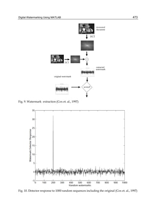
![Engineering Education and Research Using MATLAB474
This algorithm, despite the previous in spatial domain, needs the original asset for
extraction. Methods like these are called “non-blind detection” (LSB was a sample of “blind
detection”). A solution for this can be setting fix mid-frequency coefficients for preserving
the watermark message (Barni & Bartolini, 2004).
3.3 Watermarking in hybrid domain
Watermarking in hybrid domain means modifying the image regarding both spatial and
spectral specifications. One popular algorithm in this domain is performing the previous
method in small blocks of the image. This could happen in 8×8 blocks which ideally match
JPEG compression to provide least distort to the message facing with JPEG compression
attack (Barni & Bartolini, 2004). Fig. 11 illustrates this method. Pixels in blue represent
intensity of middle frequencies in the image and are most suitable for carrying message
data. The code has not been brought here because it is simply performing spread spectrum
algorithm in separate smaller blocks.
Fig. 11. Block-based hybrid method (recreated from Barni & Bartolini, 2004)
Another famous example of this is “Discrete Wavelet Transform” abbreviated as DWT. For
bringing an image to the wavelet domain one can easily use the “dwt2” command:
[bA,bH,bV,bD] = dwt2(A, ‘wname’);
In which “wname” is the type of the filter you prefer to use as wavelet decomposition and
reconstruction filters. This can be among the filter families of Daubechies (‘db1’), Coiflets
(‘coif1’), Symlets (‘sym2’), Discrete Meyer (‘dmey’), Biorthogonal (‘bior1.1’), and Reverse
Biorthogonal (rbio1.1). The option is also provided that you can use your own defined filters:
Lo_D = [1 2 1]/4; % LP Decomposition Filter
Hi_D = [1 -2 1]/4; % HP Decomposition Filter
[bA,bH,bV,bD] = dwt2(A, Lo_D, Hi_D);
The same story is true about the inverse transform:
A = idwt2(bA,bH,bV,bD, 'wname')
Or
Lo_R = [-1 2 6 2 -1]/8; % LP Reconstruction Filter
Hi_R = [1 2 -6 2 1]/8; % HP Reconstruction Filter
B = idwt2(bA,bH,bV,bD, Lo_R, Hi_R);](https://image.slidesharecdn.com/engineeringeducationandresearchusingmatlab-160628213608/85/Engineering-education-and_research_using_matlab-484-320.jpg)
![Digital Watermarking Using MATLAB 475
The output decomposed matrices of “dwt2” are of class “double” and contain negative or
above 255 values. Hence, there should be some mappings if you tend to display them. The
result is provided in Fig. 12. In the code, the maximum value for sub-bands is set to 60
which is mapped to 255. This is because they have tiny values comparing the LL image.
[bA,bH,bV,bD] = dwt2(A,'bior1.1');
B=[bA,bH;bV,bD];
subplot(2,2,1);
imshow(abs(bA),[]);
subplot(2,2,2);
imshow(abs(bH),[0 60]);
subplot(2,2,3);
imshow(abs(bV),[0 60]);
subplot(2,2,4);
imshow(abs(bD),[0 60]);
Fig. 12. Single level wavelet decomposition](https://image.slidesharecdn.com/engineeringeducationandresearchusingmatlab-160628213608/85/Engineering-education-and_research_using_matlab-485-320.jpg)
![Engineering Education and Research Using MATLAB476
Watermarking usually takes place in sub-bands. Just like the spread spectrum method,
largest coefficients can be modified according to a similar equation to (1). Another solution
is to change LSBs of these values (Vatsa et. al., 2006).
4. Evaluation of watermarking methods
Several Functions are used to qualify the watermarking algorithm, examining tests on the
resulted watermarked image.
4.1 Imperceptibility
The imperceptibility of the watermark is tested through comparing the watermarked image
with the original one. Several tests are usually used in this regard.
4.1.1 MSE
Mean Squared Error (MSE) is one of the earliest tests that were performed to test if two
pictures are similar. A function could be simply written according to equation (3).
( )
2
*
1
1
. .
n
i i
i
M S E X X
n =
= −∑ (3)
function out = MSE (pic1, pic2)
e=0;
[m,n]=size(pic1);
for i=1:m
for j=1:n
e = e + double((pic1(i,j)-pic2(i,j))^2);
end
end
out = e / (m*n);
end
4.1.2 PSNR
Pick Signal to Noise Ratio (PSNR) is a better test since it takes the signal strength into
consideration (not only the error). Equation (4) describes how this value is obtained.
2
1010.log lMAX
PSNR
MSE
⎛ ⎞
= ⎜ ⎟⎜ ⎟
⎝ ⎠
(4)
function out=PSNR(pic1, pic2)
e=MSE(pic1, pic2);
m=max(max(pic1));
out=10*log(double(m)^2/e);
end
4.1.3 SSIM
The main problem about the previous two criteria is that they are not similar to what
similarity means to human visual system (HVS). Structural Similarity (SSIM) is a function](https://image.slidesharecdn.com/engineeringeducationandresearchusingmatlab-160628213608/85/Engineering-education-and_research_using_matlab-486-320.jpg)


This chapter discusses modeling and simulating multiphase electrical machines in Matlab/Simulink. It begins with an overview of different multiphase winding configurations. It then introduces the vector space decomposition (VSD) method for unified modeling of various multiphase schemes. The VSD approach involves a geometric transformation to map actual windings to a conventional model, followed by a decoupling transformation. This allows developing the VSD theory for the conventional model independently of actual machine topology. Examples are provided of mapping different multiphase arrangements to the conventional model to enable unified simulation in Matlab/Simulink.


![[Steven karris] introduction_to_simulink_with_engi](https://cdn.slidesharecdn.com/ss_thumbnails/stevenkarrisintroductiontosimulinkwithengibooksee-160426081331-thumbnail.jpg?width=640&height=640&fit=bounds)