Chapter_11_memory_system this is part of computer architecture.pptx
1.
1
The Memory System
ProcessorDesign
The Language of Bits
Prof. Smruti Ranjan Sarangi
IIT Delhi
Basic Computer Architecture
PowerPoint Slides
Chapter 11: The Memory System
2.
Download the pdfof the book
www.basiccomparch.com
videos
Slides, software, solution manual
Print version
(Publisher: WhiteFalcon, 2021)
Available on e-commerce sites.
The pdf version of the book and
all the learning resources can be
freely downloaded from the
website: www.basiccomparch.com
2nd
version
3.
3
Outline
Overview ofthe Memory System
Caches
Details of the Memory System
Virtual Memory
4.
4
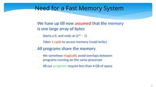
Need for aFast Memory System
We have up till now assumed that the memory
is one large array of bytes
Starts a 0, and ends at (232
– 1)
Takes 1 cycle to access memory (read/write)
All programs share the memory
We somehow magically avoid overlaps between
programs running on the same processor
All our programs require less than 4 GB of space
5.
5
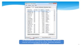
All the programsrunning on my machine. The CPU of
course runs one program at a time. Switches between
programs periodically.
6.
6
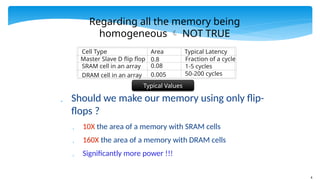
Regarding all thememory being
homogeneous NOT TRUE
Should we make our memory using only flip-
flops ?
10X the area of a memory with SRAM cells
160X the area of a memory with DRAM cells
Significantly more power !!!
Cell Type Area Typical Latency
Master Slave D flip flop 0.8 Fraction of a cycle
SRAM cell in an array 0.08 1-5 cycles
DRAM cell in an array 0.005 50-200 cycles
Typical Values
7.
7
Tradeoffs
Tradeoffs
Area,Power, and Latency
Increase Area → Reduce latency, increase power
Reduce latency → increase area, increase power
Reduce power → reduce area, increase latency
We cannot have
the best of all worlds
8.
8
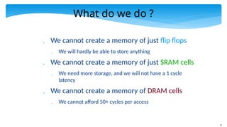
What do wedo ?
We cannot create a memory of just flip flops
We will hardly be able to store anything
We cannot create a memory of just SRAM cells
We need more storage, and we will not have a 1 cycle
latency
We cannot create a memory of DRAM cells
We cannot afford 50+ cycles per access
9.
9
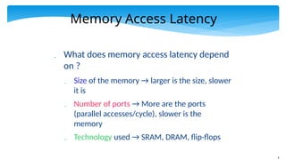
Memory Access Latency
What does memory access latency depend
on ?
Size of the memory → larger is the size, slower
it is
Number of ports → More are the ports
(parallel accesses/cycle), slower is the
memory
Technology used → SRAM, DRAM, flip-flops
10.
10
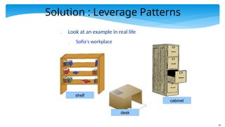
Solution : LeveragePatterns
Look at an example in real life
Sofia's workplace
desk
shelf
cabinet
11.
11
A Protocol withBooks
* Sofia keeps the
* most frequently accessed books on her desk
* slightly less frequently accessed books on the shelf
* rarely accessed books in the cabinet
* Why ?
* She tends to read the same set of books over and
over again, in the same window of time → Temporal
Locality
12.
12
Protocol – II
If Sofia takes a computer architecture course
She has comp. architecture books on her desk
After the course is over
The architecture books go
back to the shelf
And, vacation planning
books come to the desk
Idea : Bring all the vacation planning books in one go. If
she requires one, in high likelihood she might require
similar books in the near future.
13.
13
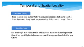
Temporal and SpatialLocality
Spatial Locality
It is a concept that states that if a resource is accessed at some point of
time, then most likely similar resources will be accessed again in the near
future.
Temporal Locality
It is a concept that states that if a resource is accessed at some point of
time, then most likely it will be accessed again in a short period of time.
14.
14
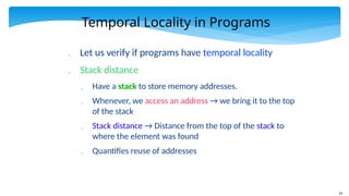
Temporal Locality inPrograms
Let us verify if programs have temporal locality
Stack distance
Have a stack to store memory addresses.
Whenever, we access an address → we bring it to the top
of the stack
Stack distance → Distance from the top of the stack to
where the element was found
Quantifies reuse of addresses
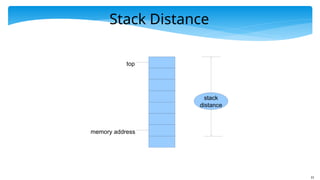
16
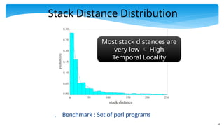
Stack Distance Distribution
Benchmark : Set of perl programs
0 50 100 150 200 250
stack distance
0.00
0.05
0.10
0.15
0.20
0.25
0.30
probability
Most stack distances are
very low High
Temporal Locality
17.
17
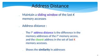
Address Distance
Maintaina sliding window of the last K
memory accesses
Address distance :
The ith
address distance is the difference in the
memory addresses of the ith
memory access,
and the closest address in the set of last K
memory accesses.
Shows the similarity in addresses
18.
18
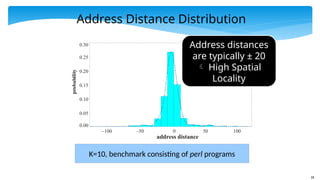
Address Distance Distribution
K=10,benchmark consisting of perl programs
0.00
0.05
0.10
0.15
0.20
0.25
0.30
probability
–100 –50 0 50 100
address distance
Address distances
are typically ± 20
High Spatial
Locality
19.
19
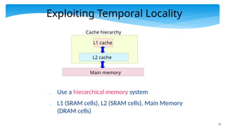
Exploiting Temporal Locality
Use a hierarchical memory system
L1 (SRAM cells), L2 (SRAM cells), Main Memory
(DRAM cells)
L1 cache
L2 cache
Main memory
Cache hierarchy
20.
20
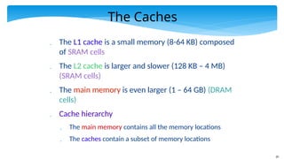
The Caches
TheL1 cache is a small memory (8-64 KB) composed
of SRAM cells
The L2 cache is larger and slower (128 KB – 4 MB)
(SRAM cells)
The main memory is even larger (1 – 64 GB) (DRAM
cells)
Cache hierarchy
The main memory contains all the memory locations
The caches contain a subset of memory locations
21.
21
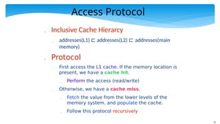
Access Protocol
InclusiveCache Hierarcy
addresses(L1) ⊏ addresses(L2) ⊏ addresses(main
memory)
Protocol
First access the L1 cache. If the memory location is
present, we have a cache hit.
Perform the access (read/write)
Otherwise, we have a cache miss.
Fetch the value from the lower levels of the
memory system, and populate the cache.
Follow this protocol recursively
22.
22
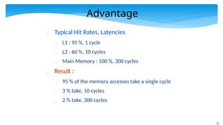
Advantage
Typical HitRates, Latencies
L1 : 95 %, 1 cycle
L2 : 60 %, 10 cycles
Main Memory : 100 %, 300 cycles
Result :
95 % of the memory accesses take a single cycle
3 % take, 10 cycles
2 % take, 300 cycles
23.
23
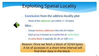
Exploiting Spatial Locality
Conclusion from the address locality plot
Most of the addresses are within +/- 25 bytes
Idea :
Group memory addresses into sets of n bytes
Each group is known as a cache line or cache block
A cache block is typically 32, 64, or 128 bytes
Reason: Once we fetch a block of 32/64 bytes.
A lot of accesses in a short time interval will
find their data in the block.
24.
24
Outline
Overview ofthe Memory System
Caches
Details of the Memory System
Virtual Memory
25.
25
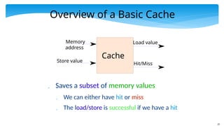
Overview of aBasic Cache
Saves a subset of memory values
We can either have hit or miss
The load/store is successful if we have a hit
Memory
address
Store value
Load value
Cache
Hit/Miss
26.
26
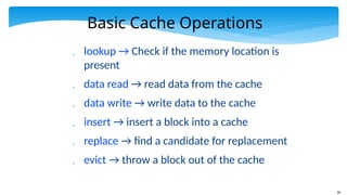
Basic Cache Operations
lookup → Check if the memory location is
present
data read → read data from the cache
data write → write data to the cache
insert → insert a block into a cache
replace → find a candidate for replacement
evict → throw a block out of the cache
27.
27
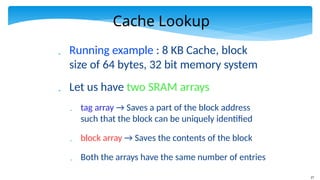
Cache Lookup
Runningexample : 8 KB Cache, block
size of 64 bytes, 32 bit memory system
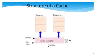
Let us have two SRAM arrays
tag array → Saves a part of the block address
such that the block can be uniquely identified
block array → Saves the contents of the block
Both the arrays have the same number of entries
28.
28
Structure of aCache
Tag array
Address
Data array
Cache controller
Store
value
Load
value
Hit / Miss
29.
29
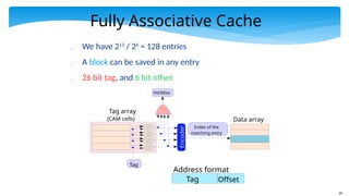
Fully Associative Cache
We have 213
/ 26
= 128 entries
A block can be saved in any entry
26 bit tag, and 6 bit offset
Tag array
(CAM cells)
Tag
Encoder
Hit/Miss
Index of the
matching entry
Data array
Tag Offset
Address format
30.
30
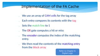
Implementation of theFA Cache
We use an array of CAM cells for the tag array
Each entry compares its contents with the tag
Sets the match line to 1
The OR gate computes a hit or miss
The encoder computes the index of the matching
entry.
We then read the contents of the matching entry
from the block array
Refer to Chapter 6:
Digital Logic
31.
31
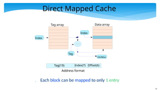
Direct Mapped Cache
Each block can be mapped to only 1 entry
Tag(19) Index(7) Offset(6)
Address format
Tag array Data array
Hit/Miss
Index
Tag
Index
32.
32
Direct Mapped Cache
We have 128 entries in our cache.
We compute the index as idx = block address % 128
We access entry, idx, in the tag array and compare the
contents of the tag (19 msb bits of the address)
If there is a match → hit
else → miss
Need a solution that is in the middle of the spectrum
33.
33
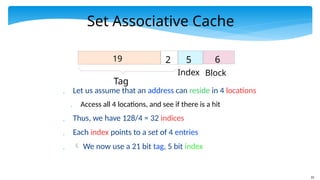
Set Associative Cache
Let us assume that an address can reside in 4 locations
Access all 4 locations, and see if there is a hit
Thus, we have 128/4 = 32 indices
Each index points to a set of 4 entries
We now use a 21 bit tag, 5 bit index
Tag
19 2 5
Index
6
Block
34.
34
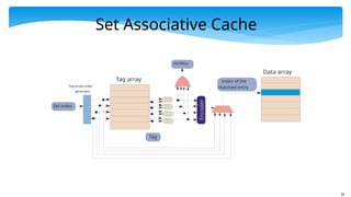
Set Associative Cache
Tagarray
Set index
Tag array index
generator
Tag
Encoder
Hit/Miss
Index of the
matched entry
Data array
35.
35
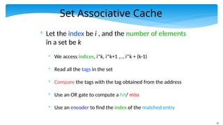
Set Associative Cache
*Let the index be i , and the number of elements
in a set be k
* We access indices, i*k, i*k+1 ,.., i*k + (k-1)
* Read all the tags in the set
* Compare the tags with the tag obtained from the address
* Use an OR gate to compute a hit/ miss
* Use an encoder to find the index of the matched entry
36.
36
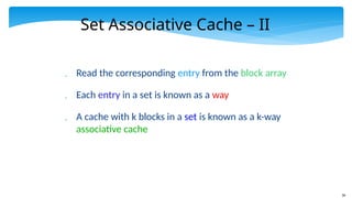
Set Associative Cache– II
Read the corresponding entry from the block array
Each entry in a set is known as a way
A cache with k blocks in a set is known as a k-way
associative cache
37.
37
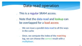
Data read operation
This is a regular SRAM access.
Note that the data read and lookup can
be overlapped for a load access
We can issue a parallel data read to all the ways
in the cache
Once, we compute the index of the matching
tag, we can choose the correct result with a
multiplexer.
38.
38
Data write operation
Before we write a value
We need to ensure that the block is present in the
cache
Why ?
Otherwise, we have to maintain the indices of the
bytes that were written to
We treat a block as an atomic unit
Hence, on a miss, we fetch the entire block first
Once a block is there in the cache
Go ahead and write to it ....
39.
39
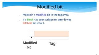
Modified bit
Maintaina modified bit in the tag array.
If a block has been written to, after it was
fetched, set it to 1.
Tag
Modified
bit
40.
40
Write Policies
Writethrough → Whenever we write to a cache,
we also write to its lower level
Advantage : Can seamlessly evict data from the cache
Write back → We do not write to the lower level.
Whenever we write, we set the modified bit.
At the time of eviction of the line, we check the
value of the modified bit
41.
41
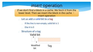
insert operation
Letus add a valid bit to a tag
If the line is non-empty, valid bit is 1
Else it is 0
Structure of a tag
Tag
Modified
bit
Valid bit
If we don’t find a block in a cache. We fetch it from the
lower level. Then we insert the block in the cache
insert operation
42.
42
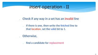
insert operation -II
Check if any way in a set has an invalid line
If there is one, then write the fetched line to
that location, set the valid bit to 1.
Otherwise,
find a candidate for replacement
43.
43
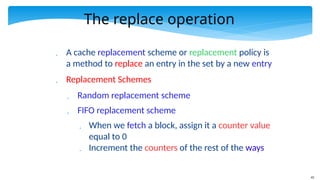
The replace operation
A cache replacement scheme or replacement policy is
a method to replace an entry in the set by a new entry
Replacement Schemes
Random replacement scheme
FIFO replacement scheme
When we fetch a block, assign it a counter value
equal to 0
Increment the counters of the rest of the ways
44.
44
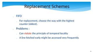
Replacement Schemes
FIFO
For replacement, choose the way with the highest
counter (oldest).
Problems :
Can violate the principle of temporal locality
A line fetched early might be accessed very frequently.
45.
45
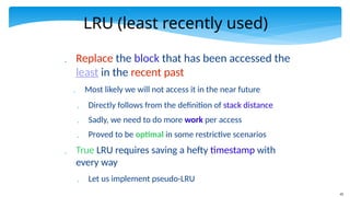
LRU (least recentlyused)
Replace the block that has been accessed the
least in the recent past
Most likely we will not access it in the near future
Directly follows from the definition of stack distance
Sadly, we need to do more work per access
Proved to be optimal in some restrictive scenarios
True LRU requires saving a hefty timestamp with
every way
Let us implement pseudo-LRU
46.
46
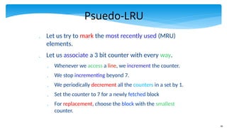
Psuedo-LRU
Let ustry to mark the most recently used (MRU)
elements.
Let us associate a 3 bit counter with every way.
Whenever we access a line, we increment the counter.
We stop incrementing beyond 7.
We periodically decrement all the counters in a set by 1.
Set the counter to 7 for a newly fetched block
For replacement, choose the block with the smallest
counter.
47.
47
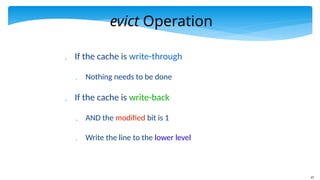
evict Operation
Ifthe cache is write-through
Nothing needs to be done
If the cache is write-back
AND the modified bit is 1
Write the line to the lower level
48.
48
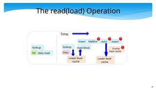
The read(load) Operation
lookup
dataread
lookup
miss
Lower level
cache
hit
replace
insert evict
read block
insert
Time
Lower level
cache
if write
back cache
49.
49
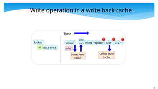
Write operation ina write back cache
lookup
data write
hit
lookup
miss
Lower level
cache
replace
insert evict
Lower level
cache
insert
write
block
Time
50.
50
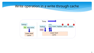
Write operation ina write through cache
lookup
data write
hit
lookup
miss
Lower level
cache
replace
insert evict
Lower level
cache
insert
write
block
Time
51.
51
Outline
Overview ofthe Memory System
Caches
Details of the Memory System
Virtual Memory
52.
52
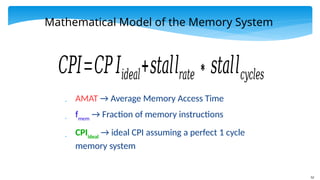
Mathematical Model ofthe Memory System
AMAT → Average Memory Access Time
fmem
→ Fraction of memory instructions
CPIideal
→ ideal CPI assuming a perfect 1 cycle
memory system
𝐶𝑃𝐼=𝐶𝑃𝐼𝑖𝑑𝑒𝑎𝑙+𝑠𝑡𝑎𝑙𝑙𝑟𝑎𝑡𝑒∗𝑠𝑡𝑎𝑙𝑙𝑐𝑦𝑐𝑙𝑒𝑠
53.
53
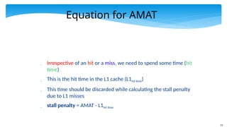
Equation for AMAT
Irrespective of an hit or a miss, we need to spend some time (hit
time)
This is the hit time in the L1 cache (L1hit time)
This time should be discarded while calculating the stall penalty
due to L1 misses
stall penalty = AMAT - L1hit time
55
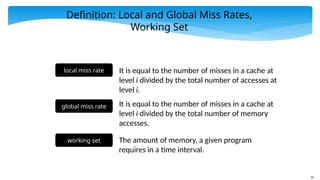
Definition: Local andGlobal Miss Rates,
Working Set
local miss rate It is equal to the number of misses in a cache at
level i divided by the total number of accesses at
level i.
global miss rate It is equal to the number of misses in a cache at
level i divided by the total number of memory
accesses.
working set The amount of memory, a given program
requires in a time interval.
56.
56
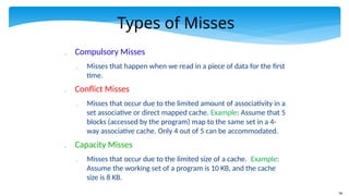
Types of Misses
Compulsory Misses
Misses that happen when we read in a piece of data for the first
time.
Conflict Misses
Misses that occur due to the limited amount of associativity in a
set associative or direct mapped cache. Example: Assume that 5
blocks (accessed by the program) map to the same set in a 4-
way associative cache. Only 4 out of 5 can be accommodated.
Capacity Misses
Misses that occur due to the limited size of a cache. Example:
Assume the working set of a program is 10 KB, and the cache
size is 8 KB.
57.
57
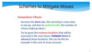
Schemes to MitigateMisses
Compulsory Misses
Increase the block size. We can bring in more data
in one go, and due to spatial locality the number of
misses might go down.
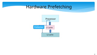
Try to guess the memory locations that will be
accessed in the near future. Prefetch (fetch in
advance) those locations. We can do this for
example in the case of array accesses.
58.
58
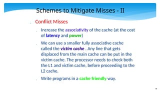
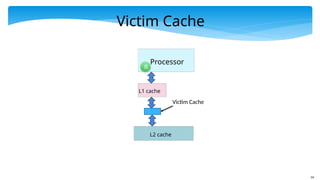
Schemes to MitigateMisses - II
Conflict Misses
Increase the associativity of the cache (at the cost
of latency and power)
We can use a smaller fully associative cache
called the victim cache . Any line that gets
displaced from the main cache can be put in the
victim cache. The processor needs to check both
the L1 and victim cache, before proceeding to the
L2 cache.
Write programs in a cache friendly way.
60
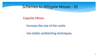
Schemes to MitigateMisses - III
Capacity Misses
Increase the size of the cache
Use better prefetching techniques.
61.
61
Some Thumb Rules
Associativity Rule → Doubling the associativity is
almost the same as doubling the cache size with
the original associativity
64 KB, 4 way ←→ 128 KB, 2 way
𝑚𝑖𝑠𝑠 𝑟𝑎𝑡𝑒∝
1
√ h
𝑐𝑎𝑐 𝑒𝑠𝑖𝑧𝑒
[𝑆𝑞𝑢𝑎𝑟𝑒 𝑅𝑜𝑜𝑡 𝑅𝑢𝑙𝑒]
62.
62
int addAll(int data[],int vals[]) {
int i, sum = 0;
for (i=0; i < N; i++)
sum += data[vals[i]];
return sum;
}
int addAllP(int data[], int vals[]) {
int i, sum = 0;
for (i=0; i < N; i++) {
__builtin_prefetch(& data[vals[i+100]] );
sum += data[vals[i]];
}
return sum;
}
Software Prefetching
Original Code
Modified Code
with
Prefetching
64
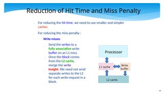
Reduction of HitTime and Miss Penalty
For reducing the hit time, we need to use smaller and simpler
caches
For reducing the miss penalty :
Write misses
Send the writes to a
fully associative write
buffer on an L1 miss.
Once the block comes
from the L2 cache,
merge the write
Insight: We need not send
separate writes to the L2
for each write request in a
block.
Processor
L1 cache
Write
buffer
L2 cache
65.
65
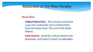
Reduction of theMiss Penalty
Read Miss
Critical Word First : The memory word that
cause the read/write miss is fetched first
from the lower level. The rest of the block
follows.
Early Restart : Send the critical word to the
processor, and make it restart its execution.
66.
66
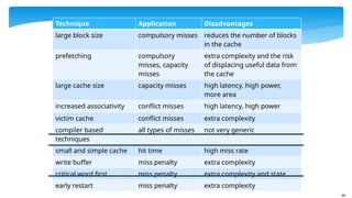
Technique Application Disadvantages
largeblock size compulsory misses reduces the number of blocks
in the cache
prefetching compulsory
misses, capacity
misses
extra complexity and the risk
of displacing useful data from
the cache
large cache size capacity misses high latency, high power,
more area
increased associativity conflict misses high latency, high power
victim cache conflict misses extra complexity
compiler based
techniques
all types of misses not very generic
small and simple cache hit time high miss rate
write buffer miss penalty extra complexity
critical word first miss penalty extra complexity and state
early restart miss penalty extra complexity
67.
67
Outline
Overview ofthe Memory System
Caches
Details of the Memory System
Virtual Memory
68.
68
Need for VirtualMemory
Up till now we have assumed that a program perceives the
entire memory system to be its own
Furthermore, every program on a 32 bit machine assumes that
it owns 4 GB of memory space, and it can access any location
at will
We now need to take multiple programs into account. The
CPU runs program A for some time, then switches to program
B, and then to program C. Do they corrupt each other’s data?
Secondly, we need to design memory systems that have less
than 4 GB of memory (for a 32 bit memory address)
69.
69
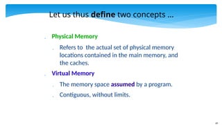
Let us thusdefine two concepts ...
Physical Memory
Refers to the actual set of physical memory
locations contained in the main memory, and
the caches.
Virtual Memory
The memory space assumed by a program.
Contiguous, without limits.
70.
70
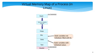
Virtual Memory Mapof a Process (in
Linux)
Header
0
0x08048000
Text
Static variables with
initialized values
Data
Static variables not
initialized, filled with 0s
Bss
Heap
Memory mapping
segment
Stack
0xC0000000
71.
71
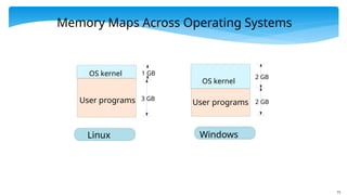
Memory Maps AcrossOperating Systems
User programs
OS kernel
3 GB
1 GB
User programs
OS kernel
2 GB
2 GB
Linux Windows
72.
72
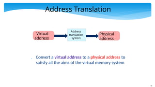
Address Translation
Converta virtual address to a physical address to
satisfy all the aims of the virtual memory system
Address
translation
system
Physical
address
Virtual
address
73.
73
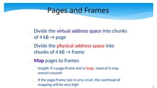
Pages and Frames
Divide the virtual address space into chunks
of 4 kB → page
Divide the physical address space into
chunks of 4 kB → frame
Map pages to frames
Insight: If a page/frame size is large, most of it may
remain unused
If the page/frame size is very small, the overhead of
mapping will be very high
74.
74
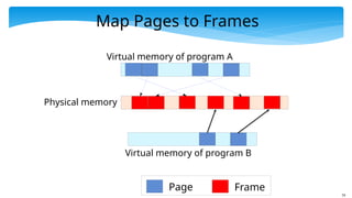
Map Pages toFrames
Virtual memory of program A
Physical memory
Page Frame
Virtual memory of program B
75.
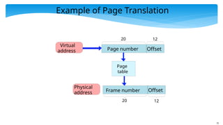
75
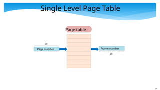
Example of PageTranslation
Page
table
Physical
address
Virtual
address Page number Offset
Frame number Offset
20 12
20 12
77
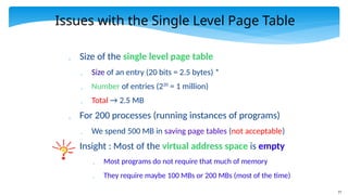
Issues with theSingle Level Page Table
Size of the single level page table
Size of an entry (20 bits = 2.5 bytes) *
Number of entries (220
= 1 million)
Total → 2.5 MB
For 200 processes (running instances of programs)
We spend 500 MB in saving page tables (not acceptable)
Insight : Most of the virtual address space is empty
Most programs do not require that much of memory
They require maybe 100 MBs or 200 MBs (most of the time)
78.
78
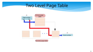
Two Level PageTable
Page number
Frame number
20
20
Primary page
table
10 10
Secondary page tables
79.
79
Two Level PageTables - II
We have a two level set of page tables
Primary and secondary page tables
Not all the entries of the primary page table point to valid secondary
page tables
Each secondary page table → 1024 * 2.5 B = 2.5 KB
Maps 4MB of virtual memory
Insight: Allocate only those many secondary page tables as required.
We do not need many secondary page tables due to spatial locality in
programs
Example: If a program uses 100 MB of virtual memory and needs 25
secondary page tables, we need a total of 2.5KB * 25 = 62.5 KB of
space for saving secondary page tables (minimal).
80.
80
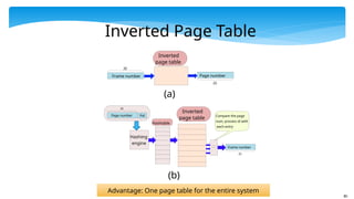
Page number
Frame number
20
20
Inverted
pagetable
Pid
Hashing
engine
Hashtable
Compare the page
num, process id with
each entry
Frame number Page number
20
20
Inverted
page table
(a)
(b)
Inverted Page Table
Advantage: One page table for the entire system
81.
81
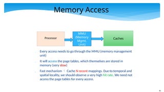
Memory Access
Processor
MMU
(Memory
Mgmt.
Unit)
Caches
Everyaccess needs to go through the MMU (memory management
unit)
It will access the page tables, which themselves are stored in
memory (very slow)
Fast mechanism Cache N recent mappings. Due to temporal and
spatial locality, we should observe a very high hit rate. We need not
access the page tables for every access.
83
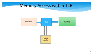
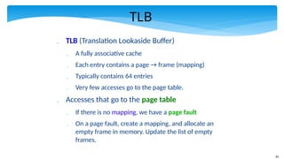
TLB
TLB (TranslationLookaside Buffer)
A fully associative cache
Each entry contains a page → frame (mapping)
Typically contains 64 entries
Very few accesses go to the page table.
Accesses that go to the page table
If there is no mapping, we have a page fault
On a page fault, create a mapping, and allocate an
empty frame in memory. Update the list of empty
frames.
84.
84
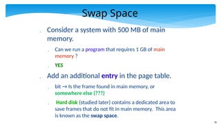
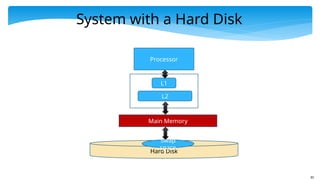
Swap Space
Considera system with 500 MB of main
memory.
Can we run a program that requires 1 GB of main
memory ?
YES
Add an additional entry in the page table.
bit → Is the frame found in main memory, or
somewhere else (???)
Hard disk (studied later) contains a dedicated area to
save frames that do not fit in main memory. This area
is known as the swap space.
85.
85
System with aHard Disk
Processor
L1
L2
Main Memory
Hard Disk
Swap
space
86.
86
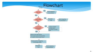
TLB hit?
Yes
Memory
access
Send mapping
toprocessor
Page table
hit?
Yes
No
Populate
TLB
No
Send mapping
to processor
Free frame
available?
No (1) Evict a frame
to swap space
(2) Update its page
table
Yes
Create/update mapping
in the page table
Populate
TLB
Send mapping
to processor
Read in the new frame
from swap space (if possible),
or create a new empy frame
Flowchart
87.
87
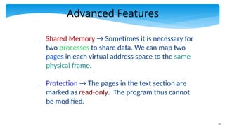
Advanced Features
SharedMemory → Sometimes it is necessary for
two processes to share data. We can map two
pages in each virtual address space to the same
physical frame.
Protection → The pages in the text section are
marked as read-only. The program thus cannot
be modified.


![61
Some Thumb Rules
Associativity Rule → Doubling the associativity is
almost the same as doubling the cache size with
the original associativity
64 KB, 4 way ←→ 128 KB, 2 way
𝑚𝑖𝑠𝑠 𝑟𝑎𝑡𝑒∝
1
√ h
𝑐𝑎𝑐 𝑒𝑠𝑖𝑧𝑒
[𝑆𝑞𝑢𝑎𝑟𝑒 𝑅𝑜𝑜𝑡 𝑅𝑢𝑙𝑒]](https://image.slidesharecdn.com/chapter11memorysystem-250217083950-28921f86/85/Chapter_11_memory_system-this-is-part-of-computer-architecture-pptx-61-320.jpg)
![62
int addAll(int data[], int vals[]) {
int i, sum = 0;
for (i=0; i < N; i++)
sum += data[vals[i]];
return sum;
}
int addAllP(int data[], int vals[]) {
int i, sum = 0;
for (i=0; i < N; i++) {
__builtin_prefetch(& data[vals[i+100]] );
sum += data[vals[i]];
}
return sum;
}
Software Prefetching
Original Code
Modified Code
with
Prefetching](https://image.slidesharecdn.com/chapter11memorysystem-250217083950-28921f86/85/Chapter_11_memory_system-this-is-part-of-computer-architecture-pptx-62-320.jpg)