School of PublicHealth
• At the end of this session students will be able to:
• Define statistical estimation
• Explain two ways of estimation
• Understand and compute two-sided and one-
sided CIs
• Compute CI for Means (single and two
population means)
• Compute CI for proportions (single and double
population proportions)
Learning objectives
2
3.
School of PublicHealth
• The procedure by which we reach a conclusion about a
population on the basis of the information contained
in a sample drawn from that population is known as
statistical inference.
• There are two ways of statistical inference;
• Estimation and
• Hypothesis testing
Estimation
3
4.
School of PublicHealth
• Estimation: is about estimating population parameters
based on sample statistics (by computation of a statistic
from sample data)
• The statistic itself is called an estimator and can be of
two types: point or interval.
• The value or values that the estimator assumes are
called estimates.
Estimation, Estimator & Estimate
4
5.
School of PublicHealth
• There are two ways to estimate population values from sample
values
– Point estimation
• using a sample statistic to estimate a population parameter
based on a single value
• e.g. if a random sample of Tigray births gave =3.5kg, and
we use it to estimate , the mean birth weight of all
Tigray births in the sampled population, we are making a
point estimation
• Point estimation ignores sampling error !
– Interval estimation
• using a sample statistic to estimate a population parameter
by making allowance for sample variation (error)
Statistical Estimation
X
5
6.
School of PublicHealth
• An estimator that represents a "single best guess" is
called a point estimator.
• When the estimate is of the form of a "range of
plausible values", it is called an interval estimator.
• Thus,
– A point estimate is of the form: [Value ],
– Whereas, an interval estimate is of the form: [ lower
limit, upper limit ]
Point Vs. Interval Estimators
6
School of PublicHealth
Sample Statistics are Estimators of Population Parameters
Sample mean,
Sample variance, S2
Sample proportion, p
Sample Odds Ratio, OŔ
Sample Relative Risk, RŔ
Sample correlation coefficient, r
µ
2
P or π
OR
RR
ρ
1. Point Estimate
• A single numerical value used to estimate the
corresponding population parameter.
X
8
9.
School of PublicHealth
• Provide an estimation of the population parameter by
defining an interval or range within which the
population parameter could be found with a given
probability or likelihood
• A confidence interval is a particular type of interval
estimator.
2. Interval estimation
9
10.
School of PublicHealth
• Give a plausible range of values of the estimate likely
to include the “true” (population) value with a given
confidence level.
• An interval estimate provides more information about
a population characteristic than does a point estimate
• Such interval estimates are called confidence
intervals.
Confidence Intervals (CIs)
10
11.
School of PublicHealth
• CIs also give information about the precision of an
estimate.
• How much uncertainty is associated with a point
estimate of a population parameter?
• When sampling variability is high, the CI will be wide
to reflect the uncertainty of the observation.
• Wider CIs indicate less certainty.
CIs…
11
12.
School of PublicHealth
• A CI in general:
– Takes into consideration variation in sample
statistics from sample to sample
– Based on observation from 1 sample
– Gives information about closeness to unknown
population parameters
– Stated in terms of level of confidence
• Never 100% sure
CIs…
12
13.
School of PublicHealth
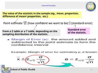
General Formula:
Point estimate (how confident we want to be) (standard error)
The value of the statistic in the sample (eg., mean, proportion,
difference of mean/ proportion, etc.)
From a Z table or a T table, depending on the
sampling distribution of the statistic.
Standard error
of the statistic.
13
14.
School of PublicHealth
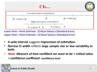
Lower limit = Point Estimate - (Critical Value) x (Standard Error)
Upper limit = Point Estimate + (Critical Value) x (Standard Error)
• A wide interval suggests imprecision of estimation.
• Narrow CI width reflects large sample size or low variability or
both.
• Note: Measure of how confident we want to be = critical value
= confidence coefficient =confidence level
CIs…
14
15.
School of PublicHealth
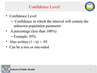
• Confidence Level
– Confidence in which the interval will contain the
unknown population parameter
• A percentage (less than 100%)
– Example: 95%
• Also written (1 - α) = .95
• Can be a two or one-sided
Confidence Level
15
16.
School of PublicHealth
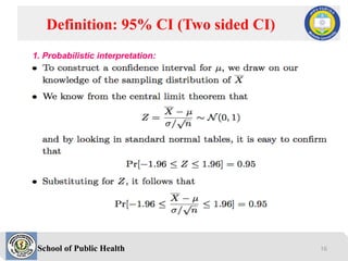
Definition: 95% CI (Two sided CI)
1. Probabilistic interpretation:
16
School of PublicHealth
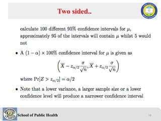
2. Practical interpretation:
• When sampling is from a normally distributed
population with known standard deviation, we are 100
(1-α) [e.g., 95%] confident that the single computed
interval contains the unknown population parameter.
Two sided…
19
20.
School of PublicHealth
• The 95% confidence interval gives an interval of
values within which there is a 95% chance of
locating the true population mean
Practical interp. 95% CI…
+1.96
n
1.96
n
X
X X
95% chance of finding within this interval
Standard
error of the
sample
mean(S.E. )
X
It quantifies the precision
of the sample mean
20
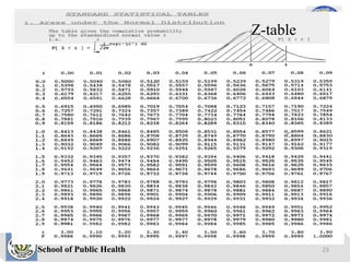
School of PublicHealth
Confidence Level to Z-Value Guide
Confidence Level Z/2 (2-Tail) Z (1-Tail)
80% = 20% 1.28 0.84
90% = 10% 1.645 1.28
95% = 5% 1.96 1.645
99% = 1% 2.575 2.325
c = 1.0-c Z(c/2) z(c-0.5)
Using statistical tables
The (1-) percent confidence interval (C.I.) for :
We want to find two values L and U between which lies with
high probability, i.e.
P( L ≤ ≤ U ) = 1-
22
School of PublicHealth
• Suppose researchers wish to estimate the mean of
some normally distributed population.
• They draw a random sample of size n from the
population and compute , which they use as a point
estimate of .
• Because random sampling involves chance, then
can’t be expected to be equal to .
• The value of may be greater than or less than .
• It would be much more meaningful to estimate by
an interval.
CI for a Population Mean
x
x
x
26
School of PublicHealth
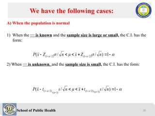
A) When the population is normal
1) When the is known and the sample size is large or small, the C.I. has the
form:
2) When is unknown, and the sample size is small, the C.I. has the form:
We have the following cases:
1
)
/
/
( )
2
/
1
(
)
2
/
1
( n
Z
x
n
Z
x
P
1
)
/
/
( )
1
(
),
2
/
1
(
)
1
(
,
)
2
/
1
( n
s
t
x
n
s
t
x
P n
n
28
29.
School of PublicHealth
B) When the population is not normal and n large (n>30)
1) When the is known the C.I. has the form:
2) When is unknown, the C.I. has the form:
CI...
1
)
/
/
( )
2
/
1
(
)
2
/
1
( n
Z
x
n
Z
x
P
29
30.
School of PublicHealth
• Suppose a researcher is interested in obtaining an
estimate of the average level of some enzyme in a
certain human population, takes a sample of 10
individuals, determines the level of the enzyme in each,
and computes a sample mean of approximately
• Suppose further it is known that the variable of interest
is approximately normally distributed with a variance
of 45. We wish to estimate the CI of . With =0.05
Example 1
22
x
30
31.
School of PublicHealth
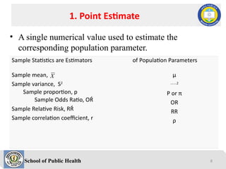
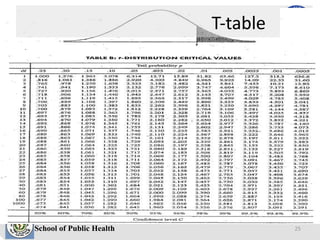
1- =0.95→ =0.05→ /2=0.025,
variance = σ2
= 45 → σ= 45,n=10,
95%confidence interval for is given by:
Z (1- /2) = Z 0.975 = 1.96 (refer table)
Z 0.975(/n) =1.96 ( 45 / 10) ≈ 4.16
22 ± 4.16) → [22-4.16; 22+4.16] → [17.84; 26.16]
Solution
22
x
1
)
/
/
( )
2
/
1
(
)
2
/
1
( n
Z
x
n
Z
x
P
31
32.
School of PublicHealth
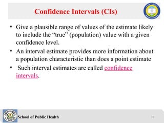
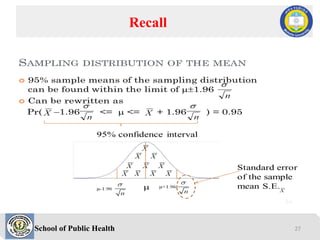
• The activity values of a certain enzyme measured in normal
gastric tissue of 35 patients with gastric carcinoma has a mean
of 0.718 and a standard deviation of 0.511.We want to
construct a 90 % confidence interval for the population mean.
Note that the population is not normal, however
n=35 (n>30) n is large and is unknown, s=0.511
1- =0.90→ =0.1→ 1-/2=0.95,
Z (1- /2) = Z0.95 = 1.645 (refer Z- table)
Z 0.95(s/n) =0.1421
0.718 ± 1.645 (0.511) / 35→ [0.576; 0.860]
Example 2
1
)
/
/
( )
2
/
1
(
)
2
/
1
( n
s
Z
x
n
s
Z
x
P
32
33.
School of PublicHealth
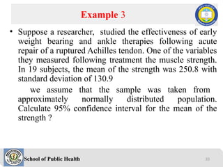
• Suppose a researcher, studied the effectiveness of early
weight bearing and ankle therapies following acute
repair of a ruptured Achilles tendon. One of the variables
they measured following treatment the muscle strength.
In 19 subjects, the mean of the strength was 250.8 with
standard deviation of 130.9
we assume that the sample was taken from
approximately normally distributed population.
Calculate 95% confidence interval for the mean of the
strength ?
Example 3
33
34.
School of PublicHealth
1- =0.95→ =0.05→ /2=0.025,
Standard deviation= S = 130.9 ,n=19
95%confidence interval for is given by:
t (1- /2),n-1 = t 0.975,18 = 2.1009 (refer t-table )
t 0.975,18(s/n) =2.1009 (130.9 / 19)=63.1
250.8 ± 63.1) → [187.7; 313.9]
Solution
8
.
250
x
1
)
/
/
( )
1
(
)
2
/
1
(
)
1
(
)
2
/
1
( n
s
t
x
n
s
t
x
P n
n
34
35.
School of PublicHealth
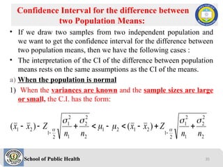
• If we draw two samples from two independent population and
we want to get the confidence interval for the difference between
two population means, then we have the following cases :
• The interpretation of the CI of the difference between population
means rests on the same assumptions as the CI of the means.
a) When the population is normal
1) When the variances are known and the sample sizes are large
or small, the C.I. has the form:
Confidence Interval for the difference between
two Population Means:
2
2
2
1
2
1
2
1
2
1
2
1
2
2
2
1
2
1
2
1
2
1 )
(
)
(
n
n
Z
x
x
n
n
Z
x
x
35
36.
School of PublicHealth
2) When variances are unknown but equal, and
the sample size is small, the C.I. has the form:
Cont’d
2
)
1
(
)
1
(
1
1
)
(
1
1
)
(
2
1
2
2
2
2
1
1
2
2
1
)
2
(
,
2
1
2
1
2
1
2
1
)
2
(
,
2
1
2
1
2
1
2
1
n
n
S
n
S
n
S
where
n
n
S
t
x
x
n
n
S
t
x
x
p
p
n
n
p
n
n
36
37.
School of PublicHealth
b) When the population is non-normal
1) When the variances are unknown and the
sample sizes are large, the C.I. has the form:
Assumptions…
2
2
2
1
2
1
2
1
2
1
2
1
2
2
2
1
2
1
2
1
2
1 )
(
)
(
n
S
n
S
Z
x
x
n
S
n
S
Z
x
x
37
38.
School of PublicHealth
The researcher team interested in the difference between serum uric
acid level in a patient with and without Down’s syndrome. In a large hospital for the
treatment of the mentally retarded, a sample of 12 individual with Down’s Syndrome
yielded a mean of mg/100 ml. In a general hospital a sample of 15 normal
individual of the same age and sex were found to have a mean value of
If it is reasonable to assume that the two population of values are normally distributed with
variances equal to 1 and 1.5, find the 95% C.I for μ1 - μ2
Solution:
1- =0.95→ =0.05→ /2=0.025 → Z (1- /2) = Z0.975 = 1.96
1.1±1.96(0.4472) = 1.1± 0.88 = ( 0.22, 1.98). We are 95% sure the true difference between means lies
within the interval 0.22 and 1.98.
Example 1
5
.
4
1
x
4
.
3
2
x
2
2
2
1
2
1
2
1
2
1 )
(
n
n
Z
x
x
38
39.
School of PublicHealth
The purpose of the study was to determine the effectiveness of an
integrated outpatient dual-diagnosis treatment program for
mentally ill subject. The authors were addressing the problem of
substance abuse issues among people with sever mental disorder.
A retrospective chart review was carried out on 50 patients, the
researcher was interested in the number of inpatient treatment
days for the disorder during a year following the end of the
program. Among 18 patient with schizophrenia, The mean
number of treatment days was 4.7 with standard deviation of 9.3.
For 10 subject with bipolar disorder, the mean number of
treatment days was 8.8 with standard deviation of 11.5. We wish
to construct 99% C.I for the difference between the means of the
populations represented by the two samples
Example 2
39
40.
School of PublicHealth
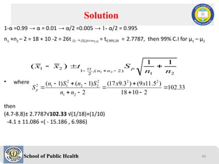
1-α =0.99 → α = 0.01 → α/2 =0.005 → 1- α/2 = 0.995
n1 +n2 – 2 = 18 + 10 -2 = 26t (1- /2),(n1+n2-2)
= t0.995,26 = 2.7787, then 99% C.I for μ1 – μ2
• where
then
(4.7-8.8)± 2.7787√102.33 √(1/18)+(1/10)
-4.1 ± 11.086 =( - 15.186 , 6.986)
Solution
2
1
)
2
(
,
2
1
2
1
1
1
)
(
2
1 n
n
S
t
x
x p
n
n
33
.
102
2
10
18
)
5
.
11
9
(
)
3
.
9
17
(
2
)
1
(
)
1
( 2
2
2
1
2
2
2
2
1
1
2
x
x
n
n
S
n
S
n
Sp
40
41.
School of PublicHealth
Remark
Independent
1. Are samples come from two
distinct populations/groups
2. have different Data sources
3. The data of the samples are
Unrelated
Independent
4.Use difference between
the 2 Sample Means:
Two different diets. Does one increase
longevity relative to the other?
• We can use independent t-test statistic
Patients assigned randomly to receive a
vaccine or placebo. Is the rate of the
disease the same in both groups, or did
the vaccine prevent disease?
Related/Dependent
1. Are samples come from related
/the same/ populations
2. Have Same/related Data Source
3. The data are either
Paired or Matched
Repeated Measures
(Before/After)
4.Use difference between each pair
of observations
Di = X1i - X2i
• We can use paired t-test statistic
RBS level of study subjects before and
after breakfast.
7 January 2026 41
)
( 2
1 x
x
42.
School of PublicHealth
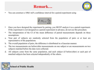
• You can construct a 100(1-a)% confidence interval for a paired experiment using
• Once you have designed the experiment by pairing, you MUST analyze it as a paired experiment.
If the experiment is not designed as a paired experiment in advance, do not use this procedure.
• The interpretation of the CI of the mean difference of paired measurements depends on these
assumptions:
a. Your pair of subjects are randomly selected from the population of pairs or at least are
representative of the populations.
b. The overall population of pairs, the difference is distributed in a Gaussian manner.
c. The two measurements are before/after measurements on one subject or are measurements on two
subjects matched before the data were collected.
d. All subjects come from the same population, and each subject (if before/after) or each pair of
matched subjects has been selected independently of the others.
Remark…
n
s
t
d d
2
/
42
43.
School of PublicHealth
Example
4.4mmHg (X1) 9.9mmHg (X2)
62.5 51.7
65.2 54.2
71.3 57.0
69.9 56.4
74.5 61.5
67.8 57.2
70.3 58.1
67.0 56.2
68. 5 58.4
62.4 55.5
VAPOR PRESSURE
The data here are on the sugar concentration
of juice in half heads of red clover kept at
different vapor pressure for 8 hours.
Construct the 99% confidence interval for
the difference in mean sugar concentration
43
44.
School of PublicHealth
Solution
xi yi di di
2
62.50 51.70
10.80 116.64
65.20 54.20
11.00 121
71.30 57.00
14.30 204.49
69.90 56.40
13.50 182.25
74.50 61.50
13.00 169
67.80 57.20
10.60 112.36
70.30 58.10
12.20 148.84
67.00 56.20
10.80 116.64
68.50 58.40
10.10 102.01
62.40 55.50
6.90 47.61
Sum
di=113.2 di
2=12824.24
The 99% confidence interval for µ1-µ2
or µd is given by:-
Therefore, the 99% confidence interval
for µ1-µ2 is (9.17, 13.47)
7 January 2026 44
.47
3
1
2.15
11.32
9.17
2.15
-
11.32
2.15
0.662
250
.
3
1
250
.
3
1
10
1
005
.
0
2
01
.
0
%
1
,
1
,
,
2
005
.
0
2
2
d
d
s
n
t
t
n
t
t
Hence
s
n
t
where
d
d
d
critical
d
45.
School of PublicHealth
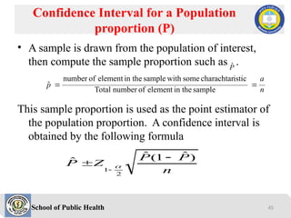
• A sample is drawn from the population of interest,
then compute the sample proportion such as .
This sample proportion is used as the point estimator of
the population proportion. A confidence interval is
obtained by the following formula
Confidence Interval for a Population
proportion (P)
n
a
p
sample
in the
element
of
number
Total
istic
charachtar
some
with
sample
in the
element
of
number
ˆ
n
P
P
Z
P
)
ˆ
1
(
ˆ
ˆ
2
1
P̂
45
46.
School of PublicHealth
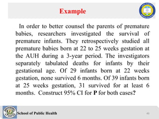
In order to better counsel the parents of premature
babies, researchers investigated the survival of
premature infants. They retrospectively studied all
premature babies born at 22 to 25 weeks gestation at
the AUH during a 3-year period. The investigators
separately tabulated deaths for infants by their
gestational age. Of 29 infants born at 22 weeks
gestation, none survived 6 months. Of 39 infants born
at 25 weeks gestation, 31 survived for at least 6
months. Construct 95% CI for P for both cases?
Example
46
47.
School of PublicHealth
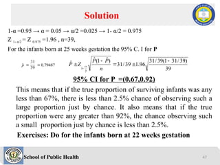
1-α =0.95 → α = 0.05 → α/2 =0.025 → 1- α/2 = 0.975
Z 1- α/2 = Z 0.975 =1.96 , n=39,
For the infants born at 25 weeks gestation the 95% C. I for P
95% CI for P =(0.67,0.92)
This means that if the true proportion of surviving infants was any
less than 67%, there is less than 2.5% chance of observing such a
large proportion just by chance. It also means that if the true
proportion were any greater than 92%, the chance observing such
a small proportion just by chance is less than 2.5%.
Exercises: Do for the infants born at 22 weeks gestation
Solution
79487
.
0
39
31
ˆ
p
39
)
39
/
31
1
(
39
/
31
96
.
1
39
/
31
)
ˆ
1
(
ˆ
ˆ
2
1
n
P
P
Z
P
47
48.
School of PublicHealth
• Two samples are drawn from two independent population of
interest, then compute the sample proportion for each sample
for the characteristic of interest. An unbiased point estimator
for the difference between two population proportions
• A 100(1-α)% confidence interval for P1 - P2 is given by:
CI for difference between two population Proportions
2
2
2
1
1
1
2
1
2
1
)
ˆ
1
(
ˆ
)
ˆ
1
(
ˆ
)
ˆ
ˆ
(
n
P
P
n
P
P
Z
P
P
48
49.
School of PublicHealth
Assumption:
The subjects are randomly selected from the population or at least are
representative of that population.
Each subject was selected independently of the rest.
The only difference between groups is exposure to the risk factor or
exposure to the treatment
Example
A researcher investigated gender differences in proactive and reactive
aggression in a sample of 323 adults (68 female and 255 males ). In
the sample, 31 of the female and 53 of the males were using internet in
the internet café. We wish to construct 99 % confidence interval for the
difference between the proportions of adults go to internet café in the
two sampled population .
CI for difference between two population
Proportions
49
50.
School of PublicHealth
1-α =0.99 → α = 0.01 → α/2 =0.005 → 1- α/2 = 0.995
Z 1- α/2 = Z 0.995 =2.58 , nF=68, nM=255,
The 99% C. I is
0.2481 ± 2.58(0.0655) = ( 0.07914 , 0.4171 )
Solution :
2078
.
0
255
53
ˆ
,
4559
.
0
68
31
ˆ
M
M
M
F
F
F n
a
p
n
a
p
M
M
M
F
F
F
M
F
n
P
P
n
P
P
Z
P
P
)
ˆ
1
(
ˆ
)
ˆ
1
(
ˆ
)
ˆ
ˆ
(
2
1
255
)
2078
.
0
1
(
2078
.
0
68
)
4559
.
0
1
(
4559
.
0
58
.
2
)
2078
.
0
4559
.
0
(
50
Editor's Notes
#13 A confidence interval is a guess (point estimate) together with a “safety net”
(interval) of guesses of a population characteristic. It has 3 components:
1) A point estimate (e.g. the sample mean)
2) The standard error of the point estimate ( e.g. SEM =σ/√ n )
3) A confidence coefficient (conf. coeff)
The “safety net” (confidence interval) that we construct has “lower” and “upper” limits
defined
Lower limit = (point estimate) – (confidence coefficient)(SE)
Upper limit = (point estimate) + (confidence coefficient)(SE)
#14 A confidence interval is a guess (point estimate) together with a “safety net”
(interval) of guesses of a population characteristic. It has 3 components:
1) A point estimate (e.g. the sample mean)
2) The standard error of the point estimate ( e.g. SEM =σ/√ n )
3) A confidence coefficient (conf. coeff)
The “safety net” (confidence interval) that we construct has “lower” and “upper” limits
defined
Lower limit = (point estimate) – (confidence coefficient)(SE)
Upper limit = (point estimate) + (confidence coefficient)(SE)


![School of Public Health
• An estimator that represents a "single best guess" is
called a point estimator.
• When the estimate is of the form of a "range of
plausible values", it is called an interval estimator.
• Thus,
– A point estimate is of the form: [Value ],
– Whereas, an interval estimate is of the form: [ lower
limit, upper limit ]
Point Vs. Interval Estimators
6](https://image.slidesharecdn.com/lecture3inferentialstatistics-estimation071853-260107181545-c7a8e236/85/Lecture-3_Inferential-statistics-Estimation_071853-pptx-6-320.jpg)


![School of Public Health
2. Practical interpretation:
• When sampling is from a normally distributed
population with known standard deviation, we are 100
(1-α) [e.g., 95%] confident that the single computed
interval contains the unknown population parameter.
Two sided…
19](https://image.slidesharecdn.com/lecture3inferentialstatistics-estimation071853-260107181545-c7a8e236/85/Lecture-3_Inferential-statistics-Estimation_071853-pptx-19-320.jpg)


![School of Public Health
1- =0.95→ =0.05→ /2=0.025,
variance = σ2
= 45 → σ= 45,n=10,
95%confidence interval for is given by:
Z (1- /2) = Z 0.975 = 1.96 (refer table)
Z 0.975(/n) =1.96 ( 45 / 10) ≈ 4.16
22 ± 4.16) → [22-4.16; 22+4.16] → [17.84; 26.16]
Solution
22
x
1
)
/
/
( )
2
/
1
(
)
2
/
1
( n
Z
x
n
Z
x
P
31](https://image.slidesharecdn.com/lecture3inferentialstatistics-estimation071853-260107181545-c7a8e236/85/Lecture-3_Inferential-statistics-Estimation_071853-pptx-31-320.jpg)
![School of Public Health
• The activity values of a certain enzyme measured in normal
gastric tissue of 35 patients with gastric carcinoma has a mean
of 0.718 and a standard deviation of 0.511.We want to
construct a 90 % confidence interval for the population mean.
Note that the population is not normal, however
n=35 (n>30) n is large and is unknown, s=0.511
1- =0.90→ =0.1→ 1-/2=0.95,
Z (1- /2) = Z0.95 = 1.645 (refer Z- table)
Z 0.95(s/n) =0.1421
0.718 ± 1.645 (0.511) / 35→ [0.576; 0.860]
Example 2
1
)
/
/
( )
2
/
1
(
)
2
/
1
( n
s
Z
x
n
s
Z
x
P
32](https://image.slidesharecdn.com/lecture3inferentialstatistics-estimation071853-260107181545-c7a8e236/85/Lecture-3_Inferential-statistics-Estimation_071853-pptx-32-320.jpg)
![School of Public Health
1- =0.95→ =0.05→ /2=0.025,
Standard deviation= S = 130.9 ,n=19
95%confidence interval for is given by:
t (1- /2),n-1 = t 0.975,18 = 2.1009 (refer t-table )
t 0.975,18(s/n) =2.1009 (130.9 / 19)=63.1
250.8 ± 63.1) → [187.7; 313.9]
Solution
8
.
250
x
1
)
/
/
( )
1
(
)
2
/
1
(
)
1
(
)
2
/
1
( n
s
t
x
n
s
t
x
P n
n
34](https://image.slidesharecdn.com/lecture3inferentialstatistics-estimation071853-260107181545-c7a8e236/85/Lecture-3_Inferential-statistics-Estimation_071853-pptx-34-320.jpg)


![Lecture 5_Analysis of Variance [ANOVA].pptx](https://cdn.slidesharecdn.com/ss_thumbnails/lecture5analysisofvarianceanova-260107181555-9a697733-thumbnail.jpg?width=640&height=640&fit=bounds)


![9.HIV[AIDS] infection for nurrse sir.ppt](https://cdn.slidesharecdn.com/ss_thumbnails/9-240616141026-5a98f126-thumbnail.jpg?width=640&height=640&fit=bounds)


