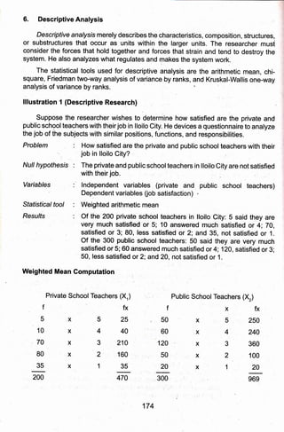
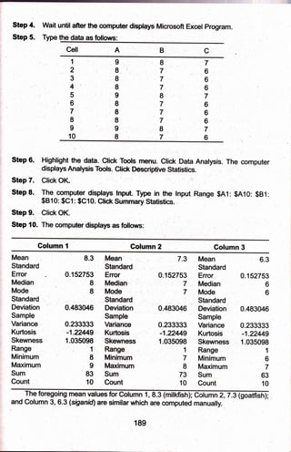
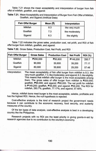
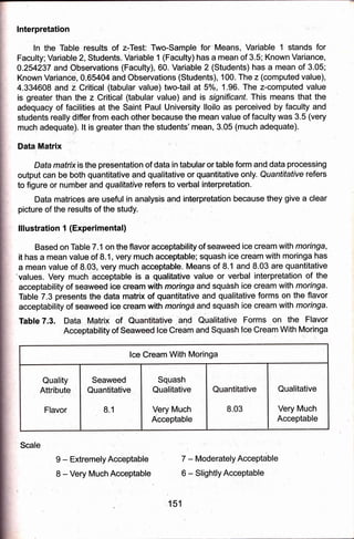
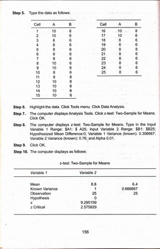
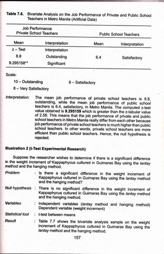
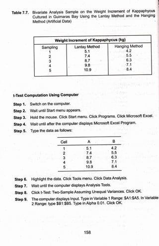
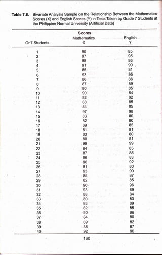
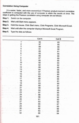
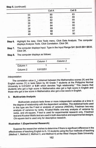
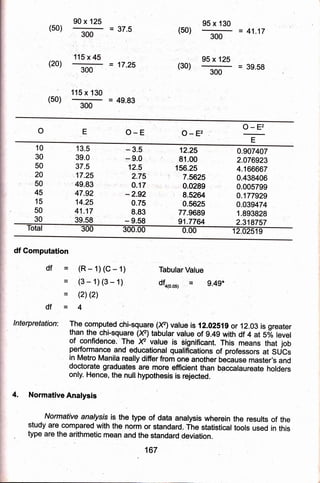
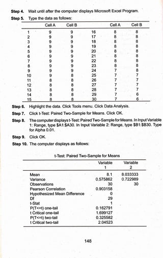
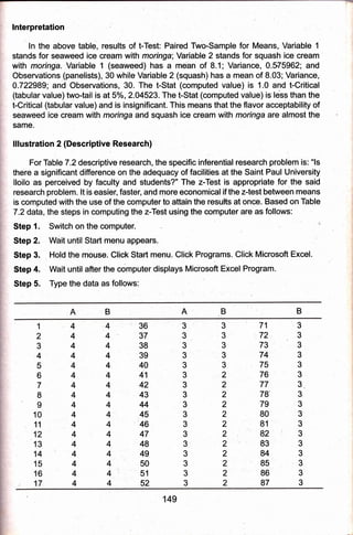
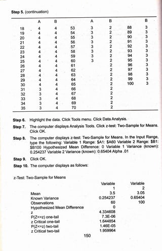
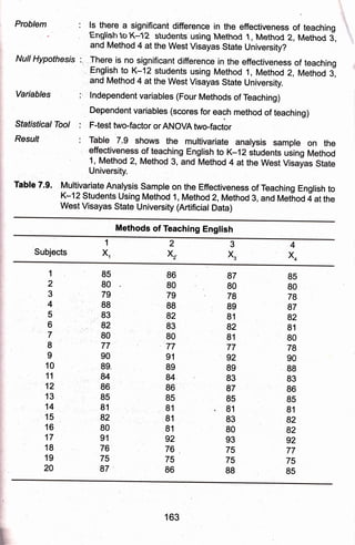
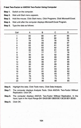
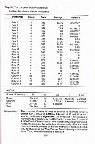
1) The document discusses data processing, statistical treatment, analysis, and interpretation of results gathered in research. It describes the basic steps of data processing as categorization, coding, and tabulation of data. 2) Two examples are provided, one experimental comparing flavor acceptability of two ice cream samples, and one descriptive comparing adequacy of university facilities. 3) The appropriate statistical tests for each example are discussed, with steps provided for calculating tests using a computer. The experimental example uses a t-test and the descriptive uses a z-test.

1. CHAPTER 7
DATA PROCESSING, STATISTICAL TREATMENT, ANALYS]S, AND
INTERPRETATION
Afterthe results have been gathered by the investigator, the next step he has to do is
to process the data into quantitative forms. Data processing involves input, throughput,
and output mechanisms. Input refers to the responses of the subject. For instance,
thE StUdY iS tit|Ed "ADEQUACY OF FACILITIES AT THE SAINT PAUL UNIVERSITY
lLOlLO." The responses or input of the subjeet of the sludy are marked as 4 for very
much adequate; 3 for much adequate; 2 for,adequate; and 1 for inadequate, which
are gathered from faculty and students..Another example of input for experimental
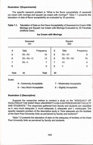
design is the result gained from the panelists'evaluation on organoleptic testing of
the quality attributes of products like colot odor, flavor, and texture in the study titled
?CCEPTABILITY OF SEAWEED ICE CREAM AND SQUASH ICE CREAM WITH
MORINGA." The responses or input are categorized as g
- extremely acceptable; g -
very much acceptable; 7 - moderately acceptable; and so on. Throughpuf involves the
statistical procedures and techniques. Outpuf indicates the results of the study which
are presented in matrix form.
Data Processing
ln data processing, quantitative and qualitative forms are involved to arrive at an
exact analysis and interpretation of the results. Data pr.ocessing consists of three basic
steps, namely, (1) categorization, (2) coding, and (3) tabulation of data.
Categoization of data is the process when data is categorized or classified into
two variables. For instance, the study conducted is on flavor acceptability of seaweed
ice cream and squash ice cream with moringa. The variables are categorized into (1)
seaweed ice cream with moringa anil (2) squash ice cream with moinga.
Co;ding, the second step of data processing of products, is done by assigning a
code to each variable such as 101 for Variable 1 or seaweed ice crearn with'rnoringa
and2A2 for Variable 2 or squash ice cream with moringa.
TabulaTion of data is the third step of data processing and is done by tallying the
results one by one. See Table 7.1 .
ln the above study, the panelists evaluated the products.organoleptically or: by
sensory evaluation using the g-point Hedonic Scale wherein 9 stands for extremely
acceptable;8, very muah acceptable;7, moderately acceptable; 6, slightly acceptabte;
5, neither-acceptable nor not acceptable; 4, slightly acceptable; 3, moderately not
acceptable;2, very much not acceptable; and 1, extremely not acceptable.
143

2. lllustration l(Experimentql) .' ., ' .' .
The specifrc research problem is"What is.the flavor,qcceptability of sepv"veed
ice cream with moringa and squash,ice qeq,m wilh moringa?" Table 7.1 presents the
tabulation of data of flavor-acceptability as evaluated by 30 panelists.
Table 7.1. Tabulation of Data on the FlavorAccep-tability of Seaweed lce Crearn With
Moringa and Squash lce Cream with,Moringa:Evaluated by 30 Paneliots
(Artificiaf Data) ,,
lce Cream with Moringa
Frequency
Squash
202
Frequency
I
15
4
2
Seaweed
101
X
9
I
7
6
30
X
I
8
7
6
10
13
7
0
illt
il
Total Total
Scale:
8 - Very Much Acceptable
7, - Moderatdly Acceptable
$ -- Slightly Acceptable
lllustration 2 (Descriptive)
Suppose the reseuarcher wisheq to conduct a the'ADEQ OF
FACILITIESATTHE SAINT PAUL UNIVERSITY ILOIL CEIVED BY LTY
AND STUDENTS." The responses gathered from faculty and students are'classified
as 4, very much adequate; 3, much adequate; 2,:adequate; and,1, inadequate. The
specific research,problem of the descriplive study ig "flow adequate are,the facilities
at the $aint Paul University lloilo as perceived by facully and.students?' 1
Table'V.2 pr:esents the tabulation of data ort the adequacy of facilities at the Saint
Paul University lldilo as percbived by faculty and students.
144

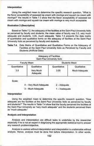
3. Table.T.2..ThbulationofDataontheAdequacy_ofFacilitiesattheSaintPau]University
Itoito as peiciiueo by Facutty andstudents (Artificial Data)
o 2 ll'l.t-lhil-
01
60 Total
dequate 2 ' Adequate
ate 1 - lnadequate
ean arethe comrnon dbscriptive statisticat
ioo]1
to gnsw!1
earch.problem' They are applicable bbth to'e;Perimental
s. After in" i"uur"tioil of data' computation is next':u$ihg
o arrive at the correci interpretation'
ticaltoolforTabteT:landTableT.2tabulationofdatais
utation below' -: '
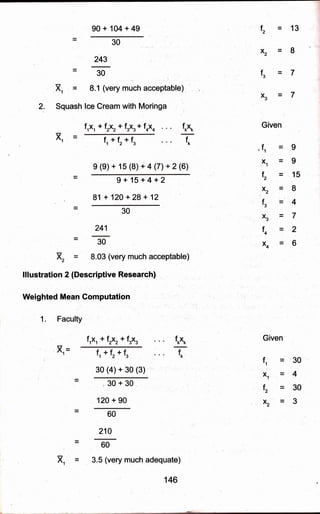
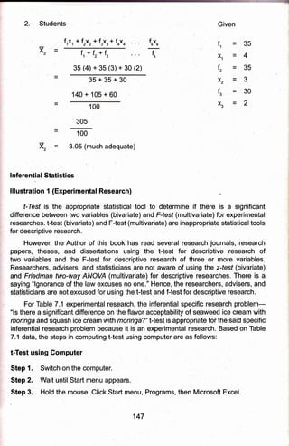
ation (EXPerimental Resea{gh)
eam with Moringa .
x, + frx. f*x* Given :
-
q*f, .'.. fk
f. = 10
1+ 13 (8) + 7 (7)
x1 '=9
10+13+7
,-,,
-.: '.

4. 90+ 104 +49
30
243
30
8.1 (very much acceptable)
lce Cream with Moringa
f,,X, + trxr+ f.X, + foXo . .
fn *fz*fs
t2
x2
fi
= 13
=8
=7
=7
x.=
Squash
x,=
x3
2
f*X* Given
fk
e (e) + 15 (8) + 4 (7) + 2 (6)
9 + 15 + 4 + 2
81 + 120+28+12
30
241
30
X, = 8.03 (very much acceptable)
lllustration 2 (Descriptive Research)
Weighted Mean Gomputation
:
1. Faculty ' :' '
frX, *trxr+frX. f*"*
X,= fl *fz+f
30 (4) + 30 (3)
,30+30
120 + 90
60
210
60
3.5 (very much adequate)
"f1
xl
f2
x2
f3
x3
f4
x4 =6
=9
=9
= 15
=8
=4
=7
=2
Given
f1
x1
t2
x2
=30
=4
=30
=3
Xl=
146

5. Students Given
f1
x1
f2
=35
=4
=35
fk
f,ix,, + f,xr* f.X, * f oxo
f1*fz*fs
35 (4) + gs (3) * 30 (2)
f*X*
35+35+30
140 + 105 + 60
100
305
100
3.05 (much adequate)
lnferential Statistics
lllustration 1 (Experimental Research)
f-Iesf is the appropriate statistical tool to determine if there is a significant
difference between two variables (bivariate) and F-fesf (multivariate) for experimental
researches. t-test (bivariate) and Ftest (multivariate) are indppropriate statisticaltools
for descriptive research.
However, the Author of this book has read several research journals, research
papers, theses, and dissertations using the t-test for descriptive research of
two var:iables and the Ftest for descriptive research of three or more variables.
Researchers, advisers, and statisticians are not aware of using the z{esf (bivariate)
and Fiedman two-way ANOVA (multivariate) for descriptive researches. There is a
saying "lgnorance of the law excuses no one." Hence, the researchers, advisers, and
statisticians are not excused for using the t-test and f-test for descriptive research.
For Table 7.1 experimental research, the inferential specific research problem-
"ls there a significant difference on the flavor acceptability of seaweed ice cream with
moringa and squgsh ice cream with moringa?" t-test is appropriate forthe said specific
inferential research problem because it is an experimental research. Based on Table
7.1 data, the steps in computing t-test using computer are as follows:
t-Test using Gomputer
Step 1. Switch on the computer.
Step 2. Wait until Start menu appears.
Step 3. Hold the mouse. Click Start menu, Programs, then Microsoft Excel.
x2=3
f3=30
x3=2
x2
147

6. Step 4. Wait until after the cbmputer displays Microsoft Excel Prog'1'66.
Step 5, Type the data as follows:
Cell A Cell B Cell A Cell B
1
2
3
4
5
6
7
8
I
10
11
12
13
14
15
8
8
8
I
8
8
B
8
8
7
7
7
7
6
6
I
I
9
I
9
I
9
I
9
8
8
I
8
8
I
,9
9
I
9
9
9
I
I
9
I
I
8
8
I
I
16
17
18
19
20
21
22
23
24
25
26
27
28
29
30
B
I
8
I
8
8
I
I
7
7
7
7
7
7
7
Step 6.
Step 7,
Step 8.
Step 9.
Step 10.
Highlight the data. Click Tools menu. Click Data Analysis.
Click t Test: Paired Two-Sample for Means. Click OK. ,
The com puter displays t-Test: Paired Two-sample for Means. I n I nput Variable
1: Range, type $A1:$A30. ln lnput Variable 2: Range, type $81:$830. Type
forAlpha 0.01.
Click OK.
The computer displays as follows:
t-Test: Paired Two-Sample for Means
Variable Variable
12
Mean
Variance ,
'
Observations
Pearson Correlation
Hypothesized Mean Difference
Df
t-Stat
P(T<=t) one-tail
t Critical onetail
P(T<=t) two-tail
t Critical two-tail
' 8.1
0.575862
30
0.903158
0
29
1
0.162791
1 .699127
0.325582
2.04523
8.033333
0.722989
30
148

7. _ :-
lnterpretation
In the above table, results of t-Test: Paired TwGSample for Means, Variable 1
stands for seaweed ice cream with moringa; Variable 2 stands for squash ice cream
with moringa. Variable 1 (seaweed) has a mean of 8.1; Variance, 0.575962; and
Observbtions (panelisls), 30 while Variable 2 (squash) has a mean of 8.03;.Variance,
0.722989; and Observations, 30. The t-Stat (computed value) is 1.0 and t-Critical
(tabular value) twotail is at 5%, 2.04523. The t-Stat (computed value) is kjss than the
t-Critical (tabular value) and is insignificant. This means that the flavor acceptability of
seaweed ice cream with moringa and squash ice cream with moringa are almost the
same.
lllustration 2 (Descriptive Research)
For Table 7.2 descriptive research, the specific inferential research problem is: "ls
there a significant difference on the adequacy of facilities at the Saint Paul University
lloilo as perceived by faculty and students?" The z-Test is appropriate,for the said
research problem. lt is easier, faster,'and more economical if the z-test between means
is computed with the use bf the computerto attain the results at once. Based on Table
7.2 data, the steps in computing the z-Test using the computer are as follows:
Step 1. Switch on the computer.
Step 2. Wait until Start menu appears..
Step 3. Hold the mouse. Ctick Start mentr. Click Programs. Click Microsoft Excel.
Step 4. Wait until after the computer displays Microsoft Excel Program.
Step 5. Type the data as follows":
A
3 71 3
3723
3733
3743
3753
2763
2773
2783
2793
2803
281 3
2823
2833
2843
2853
2863
2873
3
3
3
3
3
3
3
3
3
3
3
3
3
3
3
3
3
1
2
3
4
5
6
7
8
9
10
11
12
13
14
15
16
17
4
4
4
4
4
4
4
4
4
4
4
4
4
4
4
4:
4
36
37
38
39
40
41
42
43
44
45
46
47
48
49
50
51
52
4
4
4
4
4
4
4
4
4
4
4
4
4
4
4
4
4
149

8. Step 5. (continuation)
3
3
3
3
3
3
3
3
3
3
3
3
3
2
2
2
2
2
2
2
2
2
2
2
2
2
2
2
2
2
2
88
8€
90
91
92
93
94
95
96
97
98
99
100
A
3
3
3
3
3
3
3
3
A
4453
4454
4455
4456
4457
4458
4459
4460
4461
4462
4463
4464
4465
3466
3467
3468
3469
3470
18
19
20
21
22
23
24
25
26
27
28
29
30
31
32
33
34
35
Step 6"
Step 7.
Step 8.
Step 9.
Step 10.
Highlight the data. Click Tools menu. Click Data Analysis.
The computer displays Analysis Tools. Click z-test: Two-Sample for Means'
Click OK.
The computer displays z-test: Two-Sample for Medns. ln the lnput Range,
type the following: Variable 1 Range: $A1: $A60 Variable 2 Rang_e: $81:
$etOO Hypothesized Mean Difference: 0 Variable 1 Variance (known):
0.254237 Variable 2 Variance (known): 0.65404 Alphq .01
Click OK.
The computer displays as follows:
z-Test: Two-Sample for Means
Mean
Known Variance
Observations
Hypothesized Mean Difference
z
P(Z<=z) one-tail
z Critical one-tail
P(Z<=z) twotail
z Crilical two-tail
150
Variable
1
,3.5
0.254237
60
0
4.334608
7.3E-06
1.644854
1.46E-05
1.959964
Variable
2
3.05
0.65404
100

9. lnterpretation ": '
in tne Table results. of z-Test: Two-sample for Means, Variable 1 stands for
Faculty; Variable 2, Students. Variable 1 (Faculty) has a mean of 3.5; Known Variance;
0.254237 and bservations (Faculty), 60: Variable 2 (Students) has a mean of 3.05;
Kno*n Varian , 0.65404 and Observations (Students), 100. The z (computed value),
4.334608 and:2 Critical (tabular value) two-tail at 5o/o, 1.96. The z-computed value
ls greater than the z Critical (tabular value) and is significant, This means that the
adeqUacy of facilities at the Saint Paul University lloilo as perceived by faculty and
students really differ from each other because the mean value of faculty was 3.5 (very
much adequate). lt is greater than the'students'mean, 3.05 (much adequate).
Data Matrix
Data matrix is the presentation of data in tabular or table form and data processing
outpqt can be bOtn quantitative and qualitative or quantitative only. Quantitative refers
to figure or ndmber and qualitafive refers to verbal interpretation.
Data matrices are useful in analysis and interpretation because they give a clear
picture of the results of the study.
lllustration 1 (Experimental)
Based on Table 7.1 on the flavor acceptability of seaweed ice cream with moringa,
it has a mean valueof 8,1, very much acceptable; squash ice cream with moringa has
a mean v,alue of Q,03, very much acceptable. Means of 8.1 and 8.03 are quantitative
'values. Very much acceptable is a qualitative value or verbal interpretation of the
acceptability of seaweed ice cream wilh moringa and squdsh ice cream with moringa.
Table 7.3 presents the data matrix of quantitative and qualitative forms on the flavor
acceptability of seaweed ice cream with moringd and squash ice cream wilh moringa.
TableT;3. Data,,[Igtril oI.Q e a4O Qu Fdrms on the Flavor
Acceptability of Sea Cream and foe Cream With Moringa
lce Cream With Moringa
Quality
Attribute
Flavor
Seaweed
Quantitative
8.1
Squash
Qualitative
Very Much
Acceptable
Qualitative
Very Much
Acceptable
I '
Extremely Acceptable
I - Very Much Acceptable
7 Moderately Acceptable
6 - Slightly Acceptable
Scale
.151

10. lnterpretation
Using the weighted mean to determine the specific research question, "What ig
the flavor acceptability of seaweed icp cream with moringa and squash ice cream with
morinEa?" the results in Tcble 7.3.show that the flavor acceptability of seaweed ice
cream w:ith moinga and squash ice creqm with moinga is very much acqeptable.
lllustration 2 (Descriptive)
Based on Table 7.2, the adequacy of the facilities at the Saint Faul University lloilo
as perceived by, faculty and students, the rnean value of faculty was 3.5, very much
adequate and students, 3.05, much adequate. Table 7.4 presents the data matrix
of quantitative and qualitative forms on the adequacy of facilities at the Saint'Paul
University lloilo as perceived by faculty and stUdents.
Table 7.4. Data Matrix of Quantitative and Qualitative Forms on'the Adequacy of
Facilities at the Saint Paul University lloilo as Perceived by Faculty and
Students (Artificial Data)
Adequacy of Facilities
Saint Paul University lloilo
Qualitative
Very MuCh
Adequate
Quantitative
3.05
Faculty Mean Students Mean
Quantitative Qualitative
Much Adequate
Scale:
2 -Adequate
1- lnadequate
lnterpretation
Using the weighted mban to determine the specific research question, "How
adequate are the facilities at the Saint Paul University lloilo as perceived by faculty
and students?" The results in Table 7.4 show that the faculty perceived the facilities at
the Saint Paul University as "very muih adeqtlate" and the students perceived them
as "much adequatei'
Analysis and lnterpretation
Analysis and interpretation are dfficult tasks to undertake by the researcher
especially if he is ngt an expert in diagnbsing the appropriate statisticaltool to answer
any research problem/objectivd.
Analysis is useless without interpretation and interpretation is unattainable without
analysis. Herrce, analysis must be'done first before interpretation. ln othei words,
152
4 - Very Much Adequate
3 - Much Adequate

11. analysis and interpretation mus! go hand in hand,in order to give meaningful regults,
lnterpretation.is important to give a cle'ar,;neaning to the research,findings.
ln analyzing the datia, stratistical techniques are used to give meaning to the
data galhered fiorn the subjecl of the study, A setrof raw data pqr se is meaningless
without interpretation, but it is given meaning once it is interpreted. For instance, a
correlation value of 0.81 is meanlngless..ll is rneaningful only if it is interpretgd as "high
relationship."
Data Analysis
Dqta analysls ip pefined aB aR Assessment of data or fact in terms of quantity,
quality attribute, trait, pattern, trend; and relationship with others, so as to answer
research questions which i4volve statisticaf techniqueb and procedures.
The squrcesin analyzing research data are specific research problems/objectives,
hypotheses, measuring instrumentsi ?nd statistical tools.
Types of Data Analysis
There are ten types of data analysis. These are (1) univariate analysis, (2) bivariate
analysis, (3)'multivariate analysis, (4) normative analysis, (5) status analysis, (6)
descriptive analysis, (7)classitication analysis, (8) evaluative analysis, (9) comparative
analysis, and (10) cost-effeictive analysis.
1. Univariate Analysis
tJnivariate analysr.s tests a single variable to determine whether the sample is
similarto the population from which it has been drawn. For instance, the researcher
wishes to determine'the effectiveness of teaching financial management by Sister
X at the Saint Paul University as perceived by Bachelor in Business Management
(BBM) students. :
lllustration
Problem
Variable
Sfafistical Toal :
How efiective is the teaching oJ Technology Livef ihood Education
(TLE) Mr. X to K-12 students at the lloilo City National High School
as perceived by K-1 2 students?
The teaching of TLE by Mr. X to K-12 students at the lloilo City
Nationat Hig'h"'school as perceived by K*12 students is not
effective.
lndependent variable (TLE)
Dependent var,iable (Perception of K-1 2 Students, Sections A, B,
and C)
Weighted mean is the statistical tool to use because the options
are very much effective or 4; much effective, 3; effective, 2; and
153
ineffective,

12. Resu/f
Gomputation of Weighted Mean
Section A
f ,fx
25 100
20 60
5 10
00
170
Ifx
Xl=
If
170
50
I
X1 = 3.4
Scale:
4 - very much effective
3 - much effective
: Table 7.5 presents' the univariate "analysis sample on the
effectiveness of teaohing TLE to K-12 students at.the lloilo City
National High School. as perceived,by Students.
x
4
3
2
1
X
4
3
2
1
Section B
ffxx
10 40 4
25753
10202
001
45 135
Ifx
xr=
135
-
-
.,
,^ -
z
2 - effective
1- ineffective
40 90
Ifx
If
x3
If
45 40
& = '2-25
Table 7.5. Univariate Analysis Sample on the Effectiveness of Teaching TLE by Mr.
X toK'12 Students atthe lloilo City National High Schoolas Perceived by
Students (Artificial Data)
154

13. c,
lnterpretation: ,The grand mean obtained is 2,88. This means that the teaehing
,9f TLE by,Mr. X to K'1 2 students at the lloilo City National High
Schoo!, as pereeived'by students was much effective. Hence,
the null hypothesis is rejected .
t
.,
'
2. Bivariate Alalysis
Bivariate analysistests how two var:iables on how they differ from each other.
The common statistical tools used in bivariate analysis are z-test, T-test, and
correlation coefficient. z-test is appropriate only in bivariate descriptive research.
T-test is applicable only in biva'riate experimental research and not in descriptive
research. Correlation coefficient is applicable both in bivariate descriptive and
exferimental research.
lllustration 1 (z-Test Descriptive Research)
Suppose the researcher wishes to determine if"there'is significant difference
between the job performance of tebchers in private and public school in Metro Manila.
Problem
Null hypothesis
Variables
Sfafistical tool
Resu/f
ls there a significant difference between the job performance of
private and public school teachers in Metro Manila?
There is no significant difference between the job performance of
private and public school teachers in Metro Manila.
J,ob performance of private school teachers'and job performance
of public school teachers ,
z-test between means
Tab'le 7.6 presents the bivariate analysis computation on the job
performance of private and public school teachers in Metro Manila.
, ., .",..
Mean Job Performbnce of Private SchoolTeachers - 8.8 '
Mean Job Performance of Public SchoolTea6hers - O.+
Gomputation of zfest Using Computer
Step 1. Switch on the comButer. l
Step 2. Wait until Start rnenu appears.
Step 3. Hold the mouse. Click Start menu, Programs, then Microsoft Excel Program.
Step 4. Wait until after the computer displays Microsoft Excel Program.
155

14. Step 5, Type the data as follows:
Cell A B Cell A
1
2
3
4
5
6
7
I
I
10
11
12
13
14
15
10
10
I
8
8
I
8
10
10
8
I
10
10
10
10
16
17
18
19
20
21
22
23
24
25
il 0.
10
I
I
'8
8
8,'
8
8
8
i,' I
6
6
6
8
6
6
6
6
6
I
6
6
6
6
6
6
6
6
6
8
I
6
6
6
Step 6.
Step 7."
Step 8.
Step 9.
Step 10.
Highlight'the data. Click Tools menu. Click Data Analysis.
The computer displays Analysis Tools. Click z{est: Two-Sample for Means.
Click OK.
The computer displays z-test: Two-Sample for Means,'Type in the lnput
Variable 1 Range: $A1: $ A25; lnput Variable 2':Range: $81: $825;
Hypothesized Mean Difference:0; Variable 1 Varignce (known): 0.306667;
Variable 2 Variance (known): 0.76;.and Alpha 0.01.
Click OK.
The computbr displays as follows:
z-test: Two-Sample for Means
Variable 1 Variable 2
Mean
Known Variance
Observation
Hypothesis
z
z Critical
8.a
1
25
,0
9.295159
2.575829
6.4
0.666667
25
156

15. Table 7.6. Bivariate Analysis on the Job Performance of PrWate,and public School
Teachers i n tr,tetro Man i la (Artifi cial,, Data )
Job Performance
Prjvate School Teachers Public School Teachers
Mean lnterpretation Mean lnterpretation
z 7 Test
g.g
9.295159**
lnterpretation
Outstanding
Significant
6.4 Satisfactory
Scale:
10 - Outstanding
$ -- Very Satisfactory
0 - Satisfactory
lnterpretation: The. me.gn job performan@ of ,private .
school teachers is g.g,
outstanding, while the mean job performance of public schooi
teachers is 6.4, satisfactory in Metro Manila. The computed z-test
value obtained is 9.295159 which is greater than the z+ibular value
he job performance of private and public
: anila reallydifferfrom each other because
schoolteachers is much higherthan public
words, private school teaihers.are'more
efficient than public school teachers. Hence, the null hypothesis is
rejected.
lll ustration 2 (t-Test Experi menta I Research)
Suppose the researcher wishes to determine if there is a significant difference
in the weight.increment of'Kappaphycus cultured in Guimaras eiy using the lantay
method and the hanging method.
Problem : ls there a significant difference in the weight increment of
lGppaphycus cultured in Guimqras Bay using i-he anfay m*-noO
and the,hangingmethod? . :,.
Nullhypothesis : fhere is no grgnificant diff.erence in the weight increment of
Kappaptrycus buturgd,in Guimaras Bay using tiu t",rtaymethod
and the hanging method.
Variables' , -:' Independeht varlables (lantay method 'and hanging method)
Dependent variable (weight increment)
Sfafilsfica/ foot : t-test between means
: Table 7.7 shows the bivariate analysis sample
increment of Kappaphycus curtured in Guimaras
lantay method and the hanging method.
157
Resu/f on the weight
Bay using the

16. I
I
Table7.7. Bivariate A,nalysis Sarnple on the'Weight, 'of ,KappaphVqus
i
Cultured in Giimaras Bay Using the Lanta and the Hanging
Method (Artificial Data) '
Wei
Sampling
1
2
3,
4
'5
Lantay Method
5.1
7.4
8.7
9.8
10.9
Hanging Method
.r' ,"',4.t2
,,,,,.' .5,,5 t
6.3
': '7.1
,8.4
,
'.
:' |.
t-Test Gomputation Using'Gomputer "
: ''
.''"
'
Step 1. Switch on the comPuter.
Step 2. Wait until Start menu appears.
rs: Gl'tc*,Miorosoft Excel. '.
Step 3. Hold the mouse. Click Star't'menu. Click Program
Step 4. Wait until after the computer displays Microsoft ExceJ'P,rOgram'
Step 5. TlPe the data as follows:
Cell A B
1 5.1 4.2
2 7.4 5,5
3 ,8.7
4 9.8 7.1
5 10.9 8.4
step 6. Highlight the data. click Tools menu. ctick Data Analysis.
Step7.Waituntilthi!computerdisplaysAnalysisTools'
Step 8. Click t-Test: Two-Sampie Assuming Unequai Variance$: Click OK' '
Step 9. The computer displays lnput. Type in Variablei Range: $A1:$A5. ln Variable
2 Range Wpe $81:$B5, Type in Alpha 0'01' Click OK'
158

17. step 10. The computer d,isplays as follows:
t-TesJ: Two-Sa m ple Assu m i n g U neq u a I Varia n ces
Variable I Variable 2
'
Mean
Variance
Observation
Hypothesis
df
t-Stat
t-Gritical
8.38
5'.047
5
0
7
'{.690219
3.499493
6.3
2.525
5
lnterpretation: The computed t-Stat or t-value is 1.690219 which is less than the
' t critical or t-tabular of- 3.499483 with dt 7 at 1 percent level of
confidence. The t-value obtained is not significant. ih[;;s that
the weight. increment of Kapp'aphycirs cultured in Griimaras Bay
using the lantay method and the hanging method are almost the
same. Thus, the null hypothesis is accepted
lllustration 3 (Gorrelation)
Suppose the investigator wishes to determine the relationship between the
Mathematics (X) scores and the English (Y) scores got by Grade 7 Students at the
Philippine Normal University-
Problem : What is the relationship between the Mathematics scores and the
English scores got by Grade 7 students at the Philippine Normal
University?
Nullhypothestb : There is no relationship between the Mathematics scores and the
English scores got by Grade 7 students at the Philippine Normal
University.
Variables : lndependent variables (Mathematics and English)
Dependent variables (Mathematics scores (X) and English scores
(Y)
: Pearson Product-Moment Conelation Coefficient (r,r)
:Ta
be
tionship
) scores
go ty.
Sfafisticatl tool
Resu/f
159

18. Table 7.8. Bivariate Analysis Sarnple on the Relationship Between theJVlathematics
scores (X) and English s (Y) in Te ken by Grade 7 Students at
the Philippine Normal Un y (Artifici ta)
Gr.7 Students
$eores'
Mathernatics
X
English
Y
1
2
3
4
5
6
7
B
I
10'
11
12
''1 3
14
15
, 16
17
18
1E
20
21
22
23
24
25
26
27
28
29
3Q
31
32
33
34
'35
36
37
38
39
'40
90
97
8B
91
85
93
86
87
80
90
82
88
84,
97
83
82
B9
81
83
80
99
84:
87
86
96
B1
s3
85
82
90 -'
93
'88 '
80
93'
82: "
g0' :
84
89
88
92
. ,85
'95
B6
90
B1
95
86
B9
' 85,
B4
's2
85
85
9B
.80,
80
85
'81
80,
81
99
85
B5
B3
92
80
'90
87
85
96
89
,84
83
'89
85
86
80
82
87
90
160

19. Gorrelation Using Computer
-lt !s
easier, fast'er, and nrgre econo.rtical if Pearson,pro{uct-moment correlation
coefficient is oomputed with the use of, computer to ittain the results at onie. The
steps in getting the Pearson conelation using computer are as follows:
Step 1.' $witch on the computer.
Step 2. Wait until Start menu appear:s.
Step 3. Hold the mouse. Clict Start menu..Click Programs. Click Microsoft Excel.
step 4. wait untilafter the computer displays Microsoft Excel program.
Step 5. Type the data as follows:
Cell A Cell B
1'
,2
3
4'
5
6
7
B
I
10
'11
12
13,
14
15
16
17
1B
' 19
20
21
22
23
,24.,
25
26
27
28,
29
30
31
32
90
97
88
91
85
93
B6
87
BO
90
82
B8
B4
97
83
82
89
81
83
80
99
84
87
B6
96
81
93
85
82
e0
93
8B
161
B5
95
86
90
B1
95
86
"89
85
B4
82
B5
85
98
80
80
85
81
80
81
99
B5
B5
83
g2
BO
90
87
85
96
89
84

20. Step 5. (continued)
Cell A Cell B
33
34
35
36
37
38
39
40
80
93
82
80
84
89
88
92
83
"t,' 89
185
" '86
, ,80
82
87
,90
steo 6. Hiqhtiqht the data. click'Tools menu. click Data Analysis' The computer
OiJpf"it. Analysis Tools. Click Correlation' Click OK'
Step 7. The computer displays lnput. Type in the lnput Range $A1:$A35:$B1:$B35'
Click OK.
Step 8. The computer displays as follows:
Column 1 Column 2
Column 1
Column2
1
0.812251
lnterpretation:
een the Mathematics scores (X) artd the
rade 7 students at the Philippine Normal
oteslhigh relationship'" This means that
tics also got a high score in English and
ihose who got a lgw score in Mathematics also got a low seore in English'
3. Multivariate AnalYsis '
Muttivariate analysis tests three or more independent variables at a time in
the degree of relationShip with the dependent variables. The statistical tools used
in this type are the F-test or analysis of variance (ANOVA), Friedman two'way
analysij of variance by ranks, Kruskal-Wallis one-way analysis of variance by
ranki, and chi-square. Ffesf is used for experimental research only. Friedman
fesf and Kruskat-Wal/is fesf are used in both descriptive and experimental designs'
Chi-square fesf is used only for descriptive research'
lllustration 1 (Experimental Research)
Suppose the researcherwishes to determine if there is significant difference in the
effectiveness of teaching English to K-l2students using the four methods of teaching
(Method 1, Method 2, M;ihod 3, and Method 4) at the West Visayas State University.
162

21. Problem : ls there a significant difference in the effectireness of teaching
, English to K-12 students' using Method 1, Method 2, Method d,
and Method 4 at the West Visayas State University?
Null Hypothesis i. .lhere is no significant difference in the effectiveness of teaching
, Engrish to K-12 students using Method 1, Method 2, Method 3,
, and Method 4 at the West Visayas State University.
Variables :' ' lndependent variables (Four Methods of reaching)
Dependent variabres (scores for each method of teaching)
Statistical Tool : . Ftest two-factor oTANOVA two-factor
Result
Table 7.9. Multivariate Analysis Sample on the Effectiveness of Teaching English to
K-12 students Using Method 1, Method 2, Method 3, and Metiod i at the
West Visayas State University (Artificial Data)
Methods of Teaching English
Subjects
3
x3
1
x1
2
xr
4
x4
1
2
3
4
5
6
7
I
I
10
11
12
13
14
15
16
17
18
19
20
85
80
79
88
83
82
80
77
90
89"
84
86
85
81
82
80
91
76
75
87
86
80
79
88
82
83
BO
77
91
89
84
86
85
81
81
81
92
76
75
86
87
80
78
89
81
82
81
77
92
89
83
87
85
81
83
80
93
75
75
88
85
80
78
87
82
81
80
78
90
88
83
86
85
81
82
82
92
77
75
85
&
163

22. F-test Two-Factor or ANOVA Two-Factor Using'Gomputer
Step 1. Switch on th,e computer.
Step 2. Wait until Start menu appears.
Step 3. Hold the mouse. Click Start menu. Glick Programs. Click Microsoft Excel.
Step 4. Wait until after the computer displays Microsoft Excel Program.
Step 5. Type the data as follows:
Cell
1
2
3
4
5'
6
7
8
9
10
11
12
13
14
15
16
17
18
19
20
85
80
79
88
83
82
80
77
90
B9
84
86
85
81
82
80
91
76
75
87
86
80
79
88
82
83
80
77
91
89
84
86
85
81
81
81
92
76
75
86
87
80
78
89
8f
82
81
77
92
89
83
87
85
81
83
8o
93
75
75
88
85
80
78
87
82
81
80
78
90
88
83
86
85
81
82
82
92
77
75
85
Step 6,
Step 7.
Step 8.
Step 9.
Highlight the'data. Click Tools mehu. Click Data Analysis.
The computer'displays Analysis Tools. Click ANOVA: Two-Factor Without
Replication. Click OK.
The computer displays ANOVA: Two-Factor Without Replication. ln the
lnput, type in the lnput Range $A1:$A20:$B1:$B20:$C1:$C20:$D1:$D20.
Click OK.
164

23. step 10. The computer displays as follows:
' ANovA: Two-Factor witnout Replication
SUMMARY Gount 'Sum Average Variance
i
n'1
,i
Row 1
Row 2
Row 3
Row 4
Row 5
Row6 .
Row 7
Row S
Row 9
Row 10
Row 11
Row 12
Row 13
Row 14
Row 15
Row 16
Row 17
Row 18
Row 19
Row 20
Column 1
Colilmn2
Column 3
Column 4
,: 343
320
31A
352
328
328
32:1
,309l
363
355
334
345
340
324
328
323
368
304
" 300
346
1 660
1662
1 666
1657
. 85 .75
80
79.5
88
82
82
80.25
77,25
. 90.75
88.75
93.5
86.25
85
, 81
82
80.75
92
76
.75
86.5
83
83.1
, 93.3
82.85
0.916667
0
0.333333
0.666667
0.666667
0,666 667
0.25
0.25
0.916667
0.25
0.333333
0.25
Q
0
0.666667
0.916667
0.666667
0,666667
.,0
1.666667
21 .36842
22.83158
28.01053
19.50263
4
4
4
4
4
4
4
4
4
4
4
4
4
4
4
4
4
,4
4
4
20
20
20
20
ANOVA
Sou,rce of Variance SS df MS F crit
Rows
Columns
Error
Total
1,714.,43i9
2.1375
28.1125
1744.688
19
3
57
I
79
90.23355 192.9546' 2.240626
0.7125
' 1.444642 4.145066
0.493202
lnterpretation. The computed'F-value for rows or subjects is 1g2.g546 which is
greater than F critical of 2.2406 or 2.24 with df 19 and 57. At 0.01
lbvel of confidence:is significant.'The computed F for'eolumns tr
four methods of teaching-is 1.444642 which'is leis tnan Fcrifical of
4. 1 45066 with df 3 and 57 at 0.01 lever of probability and is insignificant.
Hence, the scores of the su or students really differ from each
other but the effectiveness I methods of'teachi -
ldh
to K-12 students at the West Msa State Univer.,ty i; it
"
sarne, Thus, the null hypothesis is accepted.
165

24. lllustration 2 (Descriptive Research)
suppose the researeher wishes to find out if thele is significant oj[9r9n99
in
tn9 jou
performance and educational qualifications of professors bt SUCs (State Universities
lnd Coleges) in Metro Manila. bhi-.quat".(X) is the appropriaJe qtatisticaltoolforthis
particular problem.
problem : ls there a significant difference in the j6'6 performance and
educationat qull ffications of professors at SUCs (State U n iversities.
ood Colleges) in Metro Manila?
Nulthypothesis : Therri is no significant differelce in the job performance and
educationalqualificationt of professors at SUCs (State Universities
and Colleges) in Metro Manila'
Variables : lndependent variables (educational qualifications)
Dependent variables fiob performance)
Statisticaltoot : Chi-square (X) .'
Resu/f . ,
. . , : Table 7.1 0 presents the sample multivariate.anblysis of descriptive
':".e"r"n
on",the job performance an! edueational qualifications
.
of professors at SUCs (State Universities and Colleges) in Metro
. Manila'
Table 7.1O. Sample Multivariate Analysis of,.-DescriPtive- Research.on'lhe Job
performance and Educational Qualifications of Profe$sorsat SUCs (Statq
' Universities and Colleges) in Metro Manila
(Artificial Data)
Job
Performance
' Educational Qualifications '
BS MA/MS DSc/EdD/PhD Total
Outstanding
Very Satisfactory
Satisfactory
10 30 50
2A 50 45
15
90
115
95
Total +5 130 , 125 ,200
Expected Frequency ComPutation
edxa5
, (10) = 13.5
, 300
115 x 125
47.92
(45) 3oo - :
90 x 130 :
(30)
166

25. 90 x 125 95 x 130
= 41 .17
(50) = 37.5 (50)
(30)
300
95 x 125
(20)
(50)
= 17.25 = 39.58
300
115 x 130
300
= 49.83
300
o-E2
o o-E o-E2
10
30
50
20
50
45
15
50
30
13.5
39.0
37.5
17,25
'49,83
47.92
14.25
41 .17
39.59
3.5.
-,9.0
12.5
2.75'
o.17
-2.92
0.7.5
g.g3
- 9.58
,12,25
91.00
156,25
: 7.5625
9.52M
0.5625
77.96g9
91 .7764
0.907407
2.076923
4.166667
0.439406
0.005799
0.177929
0.039474
1.gg3g2g
2.319757
Total 300 300.00 0.00 12.02519
df Computation
df=
lnterpretation: The computed chlsq_u1re 0c) value is ,12.02s1g or 12.03 is greater
then the chi-square (x) tabular value of 9.49 with df 4 at 5% bvel
of confidence.'The.x value is iignificant, This r""ni that job
performance and educationar quarifications of professors at sUbs
in Metro Manila really differ froni one another because master,s and
doctorate graduates are more efficient than baccalaureate holders
only. Hence, the null,hypothesis is rejected.
4. Normative Analysis
Normative analysisis the type of data analy,sis wherein the results of the
study are compared with the norm or standardr The statistical tools used in this
. type are the arithmetic mean and the standar-d deviation.
Tabular Value
dfoto.ou) = 9.4g*
df=
167

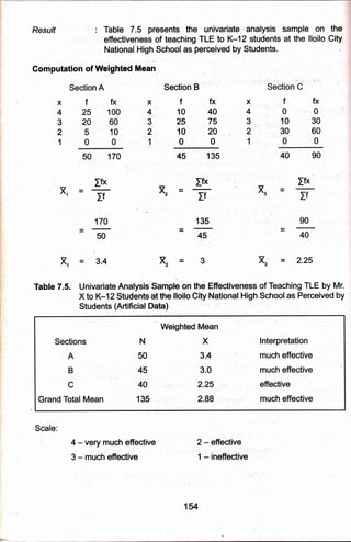
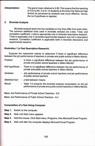
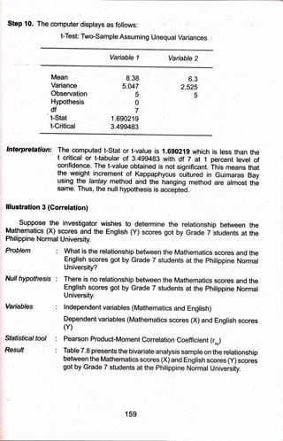
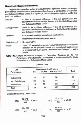
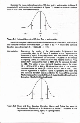
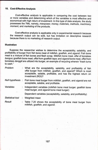
26. lllustration
Suppose the researcher wishes to conduct a study_on
]vlathelatics
aciievement
of Cr"aOe Z students at the Department of Education (DepEd) in Dipolog District; An
achievement test is used,as the mbasuring instrument to ga ed on the
Li"nr oithe test, the r,eseaichgr comparet tn" resultS with t d national
norm.
Problem : ls the Mathematics achievement of Grade 7 students at the
Department of Education (DepEd) in Dipolog District within the
regional and national norms?
N u II h vp othesis :
ffi "
IligiTi[T";ff ",ffi $,:l fiXffn I $[1'. lT",1.i'*'
'the regional ard national nonns'
Variables : lndependent variables (Mathematics regional and national norms)
Dependent varjables (Mathenratics test results)
Sfafistical fools :
Resu/f , :
Arithmetic mean and standard deviation
Table T .11 shows a mative a,nalysis on Mathernatics
achievement of Gra at the Department of Education
(DepEd) in Dipolog District.
Table 7.11. Sample Normative Analysis on Mathematics Achievement of Grade'
7:students at theDepartment.oJ Edr.rcation (DepEd) in Dipolog Distilct
(Artificial Data)
Pupils Score Pupils Score
1
2
3
4
5
6
7
I
I
10
11
12
13
14
15
16
17
18
19
20
,90
80
86
82
77
78
.84
87;
,81
91
89
83'
79
88
86
84
89
g5.
79:'
i1
76
21
22
23
24
25
26
27
2,8
29
30
31
,32
33
34
35
36
37
38
39'
40
85
88
78
75
88
89
83
85
76
88
84
80
83
81
76
80
83
77
78
75
168

27. Gomputation of Mean and;Stindardr Ddviatioh UsiFrg Gomputer
Step 1. Switch on the computer.
Step 2. Wait until Start menu appears.
Step 3" Hold the mouse. Click Start menu. Click Programs. Click Microdoft Excel.
Step 4. Wait until after the computer displays Microsoft Excel program.
Step 5. Type the data as follow.s:
Gell A Cell A Ceil A
:
Step Q. Highlight,thedata. Click l-oolsrmenu. Cl,ick Data Analysis,
Step 7. The computer displaysAnalysis Tools. Click Descriptive Statistics. Click OK.
Step 8, The comButer d,isplays,lnpul.:Typein the input Range: $it'$n+0.
Step 9. Click Summary Statistics. Click OK. , '.
Step 10. The computer displays as follows:
Column 1
Mean , 82.65
Median 83
Mode " 83
4.692492 :
Standard Deviation
- Sample Variance , '
21 .92564
Range 16
, Minimum 75
Sum 3306
169

28. Suppose the rnean national norm in a 110-item test in Mathgmatics to Grade 7
students is 80'and the standard deviation is 4. Figure 7.1 shows the assumed national
norm in a 11O-item test in Mathematics.
80 +1SD
x
Figure 7.1. National Norm of a-11O-ltem Test in Mathematics:
Based on the presumed national norm in Mathematics for Grade 7, the value of
one standard deviation above the mean (X + 1SD) is 80 + 4 =- 94 and one standard
deviation below the mean (X - 1SD) is 80 - 4 = 76.
lnterpretation: Comparing the results of the Mathematics Achievement test
' presumably taken by 40 Grade 7 students at the Department'of
Education (DepEd) in Dipdlog District with the national norm; the
Mathematics achievement of 40 Grade 7 students at the DepEd
in Dipolog District is a little bit above the national norm or "very
satisfactort''because the mean is 82.65 and the standard deviation
i14.68. The value of one standard deviation above the mean
(X * 1SD) is 82.65 + 4.68 = 87.33 and the vqlug of one standard
deviation below.the mean (X - 1SD) is 82.65 - 4.68 = 77.97. Thus,
the null hypothesis is ;'ejected; Figure 7.2 presents the mean and
one dtandard deviation above and below the mean of the assumed
Mathematics achievement of Grade 7 students at the Department of
Education (DepEd) in Dipolog Dlstrict. ,
Mean and One Standard Deviation Above and Below the Mean of
the Assumed Mathernatics Achievement of Giade 7 Students at the
Department of Education (DepEd) in Dipolog Districl
170
,-1 SD
82S5 +1SD
t-*
Figure 7.2.

29. 5. status Ai"ly:i"
Sfafus analysisstresses real facts relating to current conditions in a'group of
'subjects chosen for study. The common statistical tools used in this type are the
arithmetic mean, standard deviation, varianc€, z-test, and chi-square.
lllustration
Suppose the researcher wishes to determine if there is a significant difference
between the scholastic achievements of Biblogy students whose economic status
belong to upper-middle class and students who belong to the middle class in certain
university.
Problem : ts there a significant O'O"r"n"" between the scholastic
achievements of Biology students whose economic status belong
to the upper-middle class and those who belong to the middle
Nurt hypothesis : ;:ji"''
':H
:ffi}l dirrerence between the schorasric
' achievements of Biology students whose economic status belong
to the upper-middle claSs and those who belong to the middle
. class in certain university?
Variables i, lndependent, variables (economic status of upper-middle and
' middle class)
Dependent variables (scholastic achievements)
i '."
Statistical Tools ^: Mean, Variance, and z-test ,. : .
Resu/f
, certain university.
Table 7.12, Sample,StatusAnalysis Between the Scholastie Achievements of Biology
Students Whose Economic Status Belong to the'Uppdr-Middle Class and
Middle Class in Certain University (Artificial Data) -
: Table 7.12 tndicrrtes the sample stalus analysis between the
. scholastic achievements of Biology students whose economic
-status
belong to the upper-middle elaSs and the middle class in
Economic Status (Glass)
Students
Upper Middle
(x.') Students
"Middle
(Xr)
1
2
3
4
5
6
7
I
85
88
84
B9
90
87
91
80
1
2
3
4
5
6
7
8
83
86
8.3
88
90
88
90
81
17 1

30. : Table 7.12. (continued)
z.Test Gomputation With ttre Use of a Gomputer . -
Step 1. Switch on the computer.
Step 2. Wait untilstart menu appears.
Step 3. Hold the-mouse. Click Start menu. Click Programs. Click tfiicrosoi Excel.
step 4. wait until after the computer disptays'Microsoft Excel pibgram.
Step 5. Type the data as follows:
Cell B
Students
Upper Middte
Students
9
10
11
12
13
14
15
t6
17
18
19
20
21
22
23
24
25
82
83
86
78
79
77
80
81
75
76
85
79
83
u
90
87
88
I
10
11
12
13
14
15
16
17
18
19
20
21
22
23
24
25
83
'.82
85
7e
78
76
81
80
76
75
84
80
81
83
89
86
88
172

31. Step 5. (continued)
A
Gell
12
13
14
t5
t6
t7
18
t9
20
21
22
23
24
,25
78
79
77
80
81
75
76
85
79
.83
u
g0
g7
88
7g
78
'76
81
80
76
75
u
80
81
83
89
86
88
Step 6.
Step 7.
Step 8.
Step 9.
Step 10. The computer displays as follows:
Highlight the data. Cli* Tciols menu. Click DataAnatysis.
The'computer disptaysAnalysis Toob. Gtic* z-bst: Two-sampre for Means.
Click OK.
The corp.puter displays z-test Two-SampE for Means. Type in the lnput,
Variable 1 Range: $A1: $A25;Variable 2 Range: $B1: $B25; Hypothesized
Mean Differencs 0;,VariaUe l:fiariance (known)l 21.76;Variable 2 Variance
(known): 19.41ffi7;Alpha: 0.01.
Clict OK. .
z-test: Two-Sampte, for Jbleans
Mean
Known Variance
Obsenration
Hypothesis
z
z Critical
Variabte I
83.49
21 .76
25
.0
0.374012
2.575929
The compqted z-test value obtained is 0.37 which is less than the
z critical or z tabular of 2.58 at f percent level of confidence and
is insignlficant. Thie.means that the saholastic achievements and
stat g to the upper+nlddle
the are almost the same.
null
: 173
lnterpre:tation:

32. 6. DescriptiveAnalysis
Descriptive analysis merely describes the characteristics, composition, structures,
or substructures that occur as:uhits within the larger units. The researcher must
consider the forces that hold together and forCes that strain and tend to destroy the
system. He also analyzes what regulates and makes the system work.
The statistical tools used for descriptive analysis are the arithmetic mean, chi-
square, Friedman two.why analysis of variance by ranks, and Kr.uskal.Wallis one-way
analysis of variance by ranks. .
lllustration 1 (Descriptive Research)
Suppose the researcher wishes to determine how satisfied are the private and
public school teachers with their job in lloilo City. He devices a questionnaire to analyze
the job of the subjects with similar positions, functions, and responsibilities.
Problem : How satisfied are.the private and public schoolteachers with their
' job in lloilo City?.
Null hypothesis : The private and public school teachers in lloilo City are not satisfied
, with their job.
Variables : lndependent variables (private and public school teachers)
Dependent variables (ob satisfaction)
Sfafistical tool : Weighted, arithmetic mean
Resu/fs : Of the 200 private school teachers in lloilo City: S said they are
very much satisfied or 5; 10 answered much satisfied or 4;70,
satisfied or 3; 80, less satisfied or 2; and 3b, not satisfied or 1.
Of the 300 public school teachers: b0 said they are verl musl.l
satisfied or 5; 60 answered much satisfied or 4;12A, satisfied o.r 3;
' 50, less satisfied or 2; and 20, not satisfied or 1.
Weighted Mean Gomputation
Private School Teachers (X.,) Public School Teachers (Xr)
x' fx
250
240
360
100
20
-
969
5
4
3
2
1
X
X
X
x
X
f
50
fx
25
40
X
X
X
X
X
t
5
10
70
80
35
5
4
3
2
1
210
160
35
60
120
50
20
300
200 470

33. School
Teachers
Weighted
Mean (X) lnterpretation
Private
Public
2.35
3.23
less satisfied
satisfied
X,| Ifx
If
470
If
969
'200 t
2.35 (less satisfied)
300.
3'.23 (satisfied)
satisfaction of private
of Private and Public
Table 7.13 presents the sample descriptive analysis on job
andpublicschoolteachersinlloiloCity"'
Table 7.13. Sample Descriptive Analysis of Job Satisfaction
School Teachers in lloilo City (Artificial Data)
Scale:
Null hypothesis
Variables
Statistical tool
Resu/f
very much satisfied
much satisfied
satisfied
less satisfied r
not satisfied
5
4
3
2
1
lnterpretation: The computed mean (X) value for private school teachers is 2.35
which means less satisfied and 3.25 mean (X)vaf ue for public school
teachers which means satisfied, This meanq private schoolteachers
in lloilo City are less satisfied with their job and public school teachers
in lloilo City are satisfied with their job. Hencq, the null hypothesis is
rejected. :
lllustration 2 (Experimental Research) :
Suppo e the researcherwishes to determine the generalacceptability ofthe quality
attributes of commercial siopao and seaweed siopao, The products arq evaluated
organoleptically by 15 trained panelists using.the.g:point Hedonic Scale (from 9 - like
extremely to 1 - dislike extremely).
Problem : What is the' general
commercial sropao and
acceptability of the quality attributes of
;seaweed siopao?
: Gommercial srbpao and seaweed siopao are not acceptable.
: lndependent variables (commerciaf srbpao and seaweed siopao)
Dependent variables (general acceptability of the quality attributes)
: Weighted Mean
: Table 7.14 shows the sample descriptive analysis on the general
aceeptability of the quality attributes of commercial slopao and
seaweed siopao.
175

34. Table 7.14. sample D99 alysis on the GeneralAece of the euality
Attributes bf al siopao and seaweed sio ificial Data)
Siopao
1
2
3
4
$
6
7
8
I
10
11
12
13
14
15
B
'9
8
I
I
9
I
I
'.,8.,
I
'''8'
8
'g
8
,,8
Scale: '
9 - extremel)/ acceptable
,i
Weighted Mean Gomputation
Commercial Siopao (X,)
f - rnoderately, accepta,,ble
.i
6 - slightly aweptablq
15
x' '=
fxfx
5x840
rcx770
Ifx
rf
110
fxfx
4x930
15
V
z
124
-
' 15
8.27
110
15
7,33
b
176

35. Table 7.15p-resents the generalacceptability of the qualitytttributes of commercial
siopao and, seaweed srbpao.
Table 7.15. alpis of the Gener:al .of the eualityAttributes
Siop o and.seawee ificial Data)
Siopao Weighted Mean Descri ptive I nterpretation
Commercial 7.33 moderately acceptable
Seaweed 8.27 very much acceptable
Scale:
I
8
.- extremely ac,ceptable
- very much acceptable.
lnterpretatlon: The. mean value obtbined :for commercial siopao is 7.33 which
means "moderately acceptable" and seaweed siopao mean value,
8.27 which means'rvery much acceptable.'Thus; the null hypothesis
is rejected because seaweed siopao is more acceptable than the
. commercial siopao.
7. ClassificationAilalysis
. C/asstfica tion anatysis is usually employed in natural science subjects such
, aS Botany, Zoology, Biology, Phycology, lchthyology, Gonchology, Mycology, and
the like, The specimens collected are classifiedfrom phylum to speciei. taxonomic
studies of plants and animals are. commgnly used classifipation analysis study.
Examples of Glassification Analysis Study : .
' L ' Taxonomic Study of Herbal Plants Found,in Zamboanga del Norte and lts
Economic lmportance.
2. Taxonomic Study of MacrobenthicAlgae Found in the Waters of Zamboanga
City and lts Economic lmportance.
3.. Tqxonomic Study of Fungi Found in llocos Norte and lts Economic
lmportance.
4. Taxonomic Study :of
.Gut-Flowers Found in Leyte and lts Relation to
Socioeconomic lmpact
' 5. Taxonomic Study of Pelagic Fishes Found in the Waters of Northern lloilo.
177
.7 moderately acceptable
6 - slightly acceptable

36. 8. Evaluative Analysis , :,-i '
Evaluative anal.ysis is a type of dafa analysis that appraises carefully thil
iworthiness of the current study. The,statistical tools commonly used in this type
are the mean, percentage, variaRce,:z-test, and Friedman two-way analysis of
' variance by ranks.
lllustration
' Suppose the.researcher wishes to evaluate if there is significant difference in the
adequacy of facilities at the Department of Education (DepEd) in Dipolog District as
perceived'by d istrict supervisor/princi pals, head teachers, and teachers.
Problem : ls there a significant difierene,e in the adequacy of facilities. at the
Department of Education (DepEd) in Dipolog District as perceived
by district supervisor/principals, head teachers, and teachers?
Null hypothesls : There is no significant differ,ence in the adequacy of facilities at the
' Department of Education (DepEd) in Dipolog District as perceived
by district supervisor/principals, head teachers, and t6achers.
Variables : lndependentvariables (facilities)
Dependent variables (adequacy of facilities)
Sfafisfi'cal fools : Weighted mean and Friedman two-way ANOVA :
Resu/f : Table 7.16.shows the sample evaluative analysis on the adequacy
' of facilities at the.Department of Education (DepEd) in Dipolog
District as perceived by district supervisor/principals, head
teachers, and teachers:
Table 7.16. Sample Evaluative Analysis on the Adequacy of Facilities at the
Department of Education (DepEd) in Dipolog District as Perceived by
District Supervisor/Principals, Head Teachers, and Teachers (Artificial
Data)
Facilities
District
Supervis orl
Principals
X FR
Head
Teachers
XFR
,Teachers
X FR
1. Classrooms 3.6 2.0 3.6 2.0 3.6 2.0
2. Textbooks 3.2 2.0 3.2 2.0 3.2 2.0
3. Reference books 3.1 2.0 3.1 2.0 3.1 2.0
4. Buildings 3.3 3.0 3.2 1.5 3.2 1.5
5. Offices 3.0 2.5 3.0' 2.5 2.8 1.0
6. Teaching Aids/Devices 3.0 2.0 3.0 2.0 2.0 3.0
7. Computers for pupils 1.7 2.0 1.7 2.0 1.7 2.0
8. Computers for teiachers 2.1 2.0 2.1 2.0 2.1 2.0
178

37. Table 7 .16. (continued)
Scale:
4 :' very much adequate 2 ., fairly adequate
3adequatel-lnadequate
Friedman Two-WayANO-VA by Ranks (X,,1 Computation
w2 12
^, (tR,F - 3N (K+1)
K(K+1
12
= L (2s6 + Bto.zs+ 600,25) - 4s(4)
45(4)
12 (2766.5) - 180
180
= 0.06666667 (2766.5)
= 184.433343 180
, X:. = 4.433343 (insignifieant at 0.05 level)
degrees of freedom (df) Computation
df = (K - 1) Tabular Value
= 3-1 dfr1o.ou1=5.99*
"df=2'
D|strict
Supervisor/,
Principals
X FR
Head
Teachers
X FR
Teachers
x FR
9. Health corner 3.1 2.5 3.1 2.5 3.0 1.0
10. Comfort rooms for teachers 3.3 3.0 3.2 2.0 3.0 1.0
11 . Comfort rooms for pupils 2.9 3.0 2.7 2.0 2.6 1.0
12. Drinking fountains 2.2 2.5 2.2 2.5 2.0 1.0
13. Canteen 3.3 2.0 3.3 2.0 3.2 2.0
14. Ventilation 3.1 3.0 3.0 1.5 3.0 1.5
15.'Water supply 3.2 2.5 3.1 1.0 3.2 2.5
Total Rank (IR,) 36 29.5 24.5
179

38. lnterpretation: uted valueis4.433343,(X,2 = .
sser ueof 5.99withdf2,at5p I
of This ntean
of Education
Di rvipor/princi
and teachers are almost the sanre. Hence, the null hlpothesis is
accepted.
9. Comparative Analysis
ln comparative'analysls, the researcher considers at least tvro entities (not
manipulated) and establishes a furmal,proedure for obtaining criGrion data on
thq basis of which he can compare and mnclude that one is better than the other.
This type of data analysis is applicable only in expqrinental research wherein
the investigator conducts an experiment to'#eiminethat one is befter than the
other.
The common statisfical tools used in this.typq
"r"
r""n, variances, and
t-Test. : .
lllustrbtion I (Experimental Researeh)
Suppose the researcher wishes to study if there is a significant:difference in the
weight incrernent of oyster cultured in the brackish water of Carmen, Cebu using the
staking method and the hanging method.
Problem : ls there a significant difference in lhe weight,increment,of oyster
cultured in at tlre brackish.wabr of Garmen, Cebu using the staking
method and the hangihg method?
Null hypothesrs : There is no significant difference'in the weight increment of oyster
ctdtured in the brad<ish waterof Carmen, Cebu using,the staking
method and the hanging method.
: les (stakilrg method and hanging rnethod)
(weight increment)
Sfafi,stical fools : Me?h, variances, and t-test
Resu/f : Table 7.17 shors the sample conparative data analysis on
the weight increment of oysfier cultured in the brackish water of
Carmen, Cebu using the staking method and the hanging method.
Variables
180

39. Table 7.17. Sarhple':Conrpar,ative Ddta Analysis on the d[reight lncrement of Oyster
Cultured in the Brackish Water of Carmen, Cebu Using the Staking
Method and thb Hanging .Mettrod (Artificiat Data )
Sampling Hang[ng Method (Xr)
1
2
3
4
5
6
7
8
8.7
10.5
12.4
15.3
18.6
25.9
30.1
35..9
4.6
5.3
6.2
7.1
8.4
9.0
9.9
10.5
t-Test Computation with the Use of Gomputer
Step 1. Switch onthe computer.
Step 2. Wait until Start menu appears.
Step 3. Hold the mouse. Click Start menu. Click Programs.'Click Microsoft Excel.
Step 4. Wait until after the computer displays Microsoft Excel Program.
Step 5. Type the data as follows:
CeII A B
1 9.7 4.6
2 10.5 j: 5.3
3 72.4 6.2
4 15.3 : 7,.1 , :
5 19.6 9.4
6_ ' 25.9 9.0
7 ' ,10.1 g.g
I 35.9 10,5
1.
Step,6. Highlight the datd. Ciick Tools rn6nu, Click Data Analysis.
Step 7. Wait until after the computer displays Analysis Tools. Click t-Test: Two-
' SarnpleAssuming UnequalVariances.Click-OK.
Step 8.. The computer displays lnput. Type in Variable 1 Range: $A1:$A8. ln Variable
2 Range: type $B1; $Bg.
Step 9. ln Alpha, type 0.01. Click OK.
Step 10. The computer: displays as follows:
1gl !

40. t-Test: Two-Sample Assuming'Unequa| V6rianGes,
Variable 2 ;
Variable 1
Mean
Variance
Observation
Hypothesis
df
t-Stat
t-Critical tw
19.6625
98.1 8554
8
0
"8
3.36 1407
3.355367
. -'- i'"i i1
"r' "'(
':
7.6125
, 4.62125
8
lnterpretation: The computed t-value obtained is 3.361407 and is greater than
the t critical or t-tabular of 3355367 with df 8 at 1 percent level;of
confidence. The computed
t' ; weight increment of oyster
Cebu really differ from e
' has heavier weight increment than the hangjpg method. Thus-, the
staking method is bettgrthan the hanging method,in:cultr.ring 6yster.
Therefore, the null hypothesis is rejeCted. ,.!,
lllustration 2 (Experimental Research)
Suppose the researcher wishes to find out if there is significdnt difference in the
flavor acceptability of Kappaphycus puto and Gracilar,ia pufo. :
Problem : ls there a significant difference in the flavor acceptability of
Kappaphycus pufo and Gracilaria puto?
Nutt hypothesis : There is no significant difference in the flavor acceptability of
Variables : fndependent variables (Kappaphycus puto and Gracilaria pufo)
Dependent variable (flavor acceptability) :
Sfafistical fools : Me?h, variance, and t-Test
Resu/f : Table 7. 1 8 shows the sample comparative analysis on the difference
in flavor acceptability of Kappaphycus puto and Gracilaria pufo
Table 7.18. Sampfe Comparative Analysis of the Difiercnce in Flavor Acceptability of
Kappaphycus Pufo and Gracilaria Puto (Artificial Data)
Trained
Panelists
Kappaphycus Puto
Gracilaria Puto
x2
I
8
7
7
9
I
8
I
1
2
3
4
F--
182

41. Table 7.18.(continued) '
Trained Kappaphycus Puto Gracilaria puto
Panelists
r Xl Xz
597
6 &7
798
886
986
10 , g
Seale: , , '
I extremely acceptable 7,
' 8 - .r vsry much acceptable 6 - slighfly acceptable
t-Test Computation'with the Use of Gomputer
Step 1. Switch on the computer.
r
Step 2. Wait until Start menu appears.
Step 3. Hold the,mouse. ClickStart menu. Click Programs. Click Microsoft Excel.
Step 4. Wait until after the computer displays Microsoft Excel program.
Step6. Type the data as follows:
Cell A B
19
29
:39
87
97
4
5
6
7
I
I
87
98
8:6
86
10 ., I
Step 6. Highlight the data. Click Tools menu. Click Data Analysis.
Step 7. Click t-'liest: Paired Two-Sample for Means. Click OK.
Step8. The computer displays Input. Type in Variable 1 Range: $A1: $A10 and
Variable 2 Range: $B1: $B10.
Step 9. Type in Alpha: 0.01. Click OK:
Step 10. The computer displays as follows:
183

42. t-Test: Paired Two-Sample for Means
Variable I Variable 2
Mean
Variance
Observation
Hypothesis
df
t-Stat
t-Critical tw
'9.'5
0.277779
10
,0
9
8.573214
3.249936
7.1
0"544444
lnterpiretation: The computed t-value obtained is 8.573214 which is greatertfian the
t-critical or t-tiabularoJ 3.249836 with'df 9 ato.01 level of confidence
cant. This means that ifference in the
abilityof lGppaphycus aputobecause
Kappaphycuspufo is than Gracilaria
puto, ln other words, lGp,paphy is better than Gracilaria
pufo. Hence, the null hypothesisi
lllustration 3 (Experimental Research)
ear0her wishes to determin" in" eff.ectivgness -of teaching
od 1 and Method 2 to Grade 9'students at tne Santa lsabi
:
Prcblem ,l ls'there a significant difference in the effectiveness of teaching
chemistry using Method 1 and Method 2 to Grade 9 students at
the Santa lsabel lnternational School?
Null hypothesis : Jhere is-no -significant difference in the effectiveness of teaching
chemistry using Method 1 and Method 2 to Grade 9 students at
the Santa lsabel lntemational School.
Variabtes : lndep6ndentvar:iables (lVlethod 1 and Method 2)
Dependent yariables (Scores in each method teaching)
Sfeflsficat tools : Mean, varianee, and t-Test
Resulf :' Table 7.19 presents the sample comparative analysis on the
: effectiveness ofleaching Chemistry using Mettod 1 and Method 2
to Grade g students at the Sanla lsabel lnlernational School.'
184

43. Table 7.19. Sample ComparativeAna[ysis on the Effectiyeness of Teaching Chemistry
Using Method 1 and Method 2 to Grade'9 Students at the Santa lsabel
lnternational School (Artificial Data)
Subjects
,Methods of Teaching. G[remistry
Method 1 (X,) Method 2 (Xr)
1
2
3
4
5
6
7 :.'
' 8'.'
I
10,
''
11
,12
13
14
15
16
17
18
19
20
21
22
23
24
25
26
27
28
29
30
88
85
89
80
90
87
81
80
84
83
"85
91
88
80
79
87
88
89
81
80
84
,86
87
':'- 89
92
89,
80
82
87
85
85
83
87
80
88
86
80
77
82
81
84
91
87
,79
75
85
86
87
78
79
83
85
86
88
92
.89
", 80
86
82
t-Test Gomputation with the use of Gomputer
. f : l
Step 1. Switch on the computer,
Step 2. Wait until Start menu appears.
Step 3. Hold ihernouse,,CtiBk,$tartrnen.g, Cljqk Prggrams. Click Microsoft Excel.
Step 4. Wdit until after'the bomputer displays Micros ft Excet program.
'Step 5. Type the data as follows:
185

44. Cell Gell A
1
2
3
4
5
6
7
.8
9
10
11
12
13
14
15
88
85
89
80
90
87
81
80
84
83
85
91
88
80
79
85.'
83,
87,
80
88
86
80
77
82
81
84
91
87
'79
75
16
17
18
19
20
21
22
'"23
24
25
26
27
28
29
30
87
B8
89
81
80
84
86
87
89
92
89
80
82
87
85
85
86
' ,'87 :
:'78,
,79
83
85
86
8q
9i2
88
76
80
86
,82
Step 6.
Step 7.
Step 8.
Step 9.
Step 10.
Highlight the data, Click Tools menu. Click Data Analysis.
Wait until the.computer displays Analysis Tools: Ciick't-Test: Paired Two-
Sample for Means. Click OK.
The computer displays lnput. Type in Variabl€ 1 Range: $A1: $A30 and in
Variable 2 Range: $B1: $B30.
Type in the Alpha, 0.01.
The computer displays as follows:
t-Test: Paired Two-Sample for Means
Variable 1 Variable 2
Mean
Variance
Observation
Hypothesis
df
t-Stat
t-Critical tw
85.2
14.64825
30
0
29
8.822917
2.756396
83.5
19.22414
30
lnterpretation'. The computed t-value obtained is 8.822817 which is significant
because. it is greater than the t-cr:itical or ttabular of 2.756386 with
dt 29 at 0.01 level of confidence, This means that the effectiveness
of teaching Chemistry.using,Jl4slhod 1 and Method 2 to Grade g
students at the Santa lsabel lnternational School really differ fiom
each other because Methqd 1 is more effective in teaching Chemistry
ln other words, Method 1 is better than Method 2. Hence, the null
hypothesis is rejected.
186
+,-

45. 10. Cost-EffectiveAnalysis
Cost-effective analysis is applicable in comparing the cost between two
or more variables and determining which of the varidbles is most effective and
economicalwith high return of investment. ln this type of data analysis, the study
possesses the 7Ms, namely, mdnpower money, mateials, methods, machinery,
moment, and marl<eting ol the products.
the
'::::ff":'ffi':ff';5
because there is no marketing
lllustration
to cash."
Problem
applicable only in experimental research because
sold, but has limitation on descriptive research
of research output.
i:
Suppose the researcher wishes to determine the acceptability, salability, and
profitability of burger from fish bone meal of milkfish, goatfish, and siganid. Fish bone
'meal is a mixture of fish bones and flesh scrap. Milkfish bone meal, offal of boneless
bangus; goatfish bone rneal, offalfrom goaffish tapa;and siganid bone meal, of-falfrom
boneless danggit are utilized into burger, an example of recycling wherein "trash turns
: What are the acceptability, salability, and profitapility of fish
offal burger from milkfish, goatfish, and siganid? Which is most,
acceptable, salable, profitable, and has the highest return on
investment (ROl)?
Null hypothesis : Fish bone meal burger from miikfish, goatfish, and siganid are not
acceptable, salable, and profitable.
Variables : lndependent variables (milkfish bone meql burge.r, goatfish bone
meal burger, and siganid bone meal burger)
Dependent variables (acceptability, salability, and profitability)
Statisticaltool : Weighted mean
Resu/f : Table 7.20 shows the acceptability of bone meal burger from
milkfish, goatfish" and siganid.
187

46. Table 7.20. Acceptability of Bone Meal 'Burger from
(Artificial Data)
and Siganid
Trained
Panelists Milkfish (4)
Fish Bone Meal ,Burger
Goatfish (Xr) , Siganid (Xr)
7
6
6
6
7
"6
6
6
7
6
I
7
7
7
8
7
7
7
I
7
9
8
8
8
I
8
8
8
9
I
1
2
3
4
5
6
7
8
I
10
Scale: i
I
, '8 ' verymuchacceptable
Weighted Mean filComputation
IMilkfish (X.') Goatfish
f
3x
7
10
x1
x1
Weighted Mean Using Gomputer
,'
rn od eratel y aoce ptab I e
slightly acbeptable
Siganid (
Iv'
X
= Ifx
If
=. 63
' 10
=' 6.3
7
6
XfX
927
856
B3
= Ifx
If
=83
10
- 8.3
fx
24
49
73
:.i
Ifx
x
73
10
7.3
X')
xfx
721
642
63
(4)
f
3,
7
10
x.
fx
3xB
7xT
10
xr=
x,
It is easier, faster, and economical if the weighted mean is computed with the use
of computer to attain the results in the wink of
.an
eye. Hence, you can save time and
effort. The steps in gefting the weighted mean using.a computer are as foliows: :,
Step 1. Switch on the computer:
Step 2. Wait until Start menu appears.
- ', I .,
Step 3. Hold the mouse. Click.Start menu. Click Programs. Click Microsoft Excel.
188

47. |
SAep t Wait ur$ll afterffre,srrrprbr-disggys Excelprogram.
Step 5. Type ttre data as blows:
Cell
ftighlight the data. Qlick Tools menu. Anatysis. The computer
disflaysAnalyssTooE Cilck D6c rti
Click OK.
The cornputer displays lnrut. Type in the tnput Range $A1: $A10: $B1:
$B10: $G1: $C10. Click Summary Statistics.
Click 0(.
The.compuFr dqplays as fdlorps:,,
B
7
6
6
6
7
6
6
6
7
6
I
7
7
7
I
7
7
7
I
7
19
28
38
48
59
68
78
88
99
108
Step 6.
Step 7.
Step 8,
Step 9"
Step,'10.
Golumn 1 Golumn2 Column 3
Mean ,
Standard
Error
Median
Mode
Standard
Deviation
Sample
Variance
Kurtosis
Skewness
Range
Minimum
Maximum
Sum
Count
9.3
0.152753
I
I
0.483046
0.233333
-1 :72449
1.035099
;"'1
I
I
'93
10
7.3
0.152753
7
7
,Mean
Standard
Enor
Median
Mode
Standard
Deviation
'sample
Variance
Kurlosid "
Skewness,
Range
Minimum
Maximum
Sum
Count
6.3
0.152753
6
6
0.493046
0.233333
-1 .22449
1.035099
1
6
7
63
10
0.233333
-1 ,22449
1.03507
7
8
73
, 10
and Column 3, 6.3 (sigand) are similar urtrich @r,cornptrted manually. :
189

48. Table 7.21 shows the rnean acceptabitity and interpretation of burger from fish
offalof milkfish, goatfish, and siganid.
Table 7.21. MeainAcceptabllity and lnterpretation of Burgerfrom Fish Offalof Milkfish,
Goatfish, and Siganid (Artificial,Data)
F'ish Offal Burger Mean (X) lnterpretation
Milkfish
Goatfibn
Siganid
8.3
7.3
6.3
like very much
like moderately
like slightly
Tabte 7.22 indicates the gross'sales, production cost, net prbfit, and ROI of fish
offai burger from milkfish, goatfish, and slganrd.
Table 7.22. Gross Sales, Production Cost; Net profit, and ROI
lnterpretation: The mean acceptability of fish offat burger frorn milkfish is 8.3, like
verymuch; goatfish, 7.3, like moderately;and siganid, 6.3, like slighfly.
This means thht milkfish offal burger,is the most acceptable among
them. The gross sales of offal burger from milkfish is F200,000;
goatfish, F90,000; and siganid, F80;000, The net profit for milkfish
is F149,f,00; goatfish, ?39,200; 'and siganid, t?29,200. The ROi for
milkfish, 293.7%: goatfish, 7l.17o/o; and siganid, ST.4gyo.
Hence, milkfish bone meal burger is the nrost acceptable, salable, profitable and
has the highest ROl. Hence, the null hypothesis is r.ejected.
Cost-efiec1ive analysis is the kind of research project the government needs
because it can contribute to the economic re@very food security, and austerity
measures of the country.
Ot
!!e ten tyOes of data analysis, cost-effective analysis is best in a developing
country like the Philippines.
Research projects with no ROI are the lqast priority in giving grants-in-aid by
research agencies due to no contribution to the country's economy.
190
Fish Offal Burger Gross Sales Net Profit Rol (%l
Milkfish
Goatfish
Siganid
7200,000
90,000
80,000
F50,900
50,900,
50,900
P149,200
39r200
29,200
293.7
77.17
57.48