Download to read offline


![No
com
m
ercialuse
Single-case data analysis: Resources
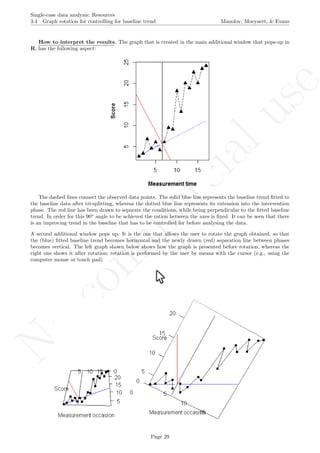
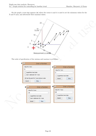
3.4 Graph rotation for controlling for baseline trend Manolov, Moeyaert, & Evans
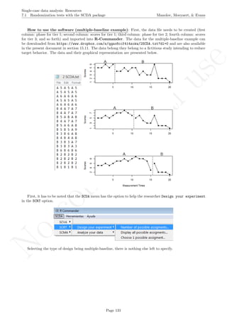
The latter two specifications are based on the information about the number of measurements and the
maximal score obtained. Given that rotating the graph is similar to transforming the data, the exact maximal
value of the Y-axis is not critical (especially in terms of nonoverlap), given that the relative distance between
the measurements is maintained.
# Number of measurements
length(score)
## [1] 19
# Maximal value needed for rescaling
max(score)
## [1] 24.2
A name is given to the axes.
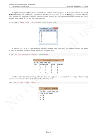
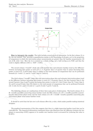
The user needs to click with the on each of the data points in order to retrieve the data and then click
Page 33](https://image.slidesharecdn.com/635a0af9-e378-45de-b512-1e1e88e419b8-160210073243/85/Tutorial-37-320.jpg)


![No
com
m
ercialuse
Single-case data analysis: Resources
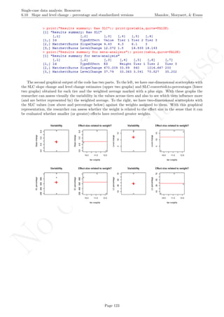
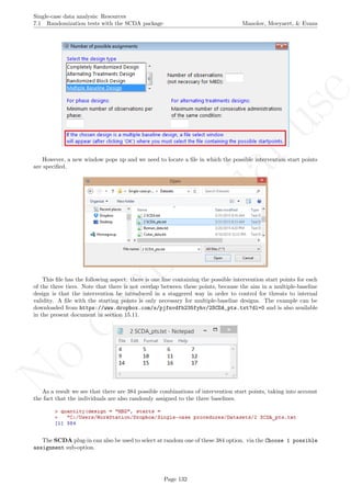
6.8 Mean phase difference - percentage and standardized versions Manolov, Moeyaert, & Evans
6.8 Mean phase difference - percentage and standardized versions
Name of the technique: Mean phase difference (MPD-P): percentage version
Authors and suggested readings: The MPD-P was proposed and tested by Manolov and Rochat (2015).
The authors offer the details for this procedure, which modifies the Mean phase difference fitting the baseline
trend in a different way and transforming the result into a percentage. Moreover, this indicator is applicable to
designs that include several AB-comparisons offering both separate estimates and an overall one. The combina-
tion of the individual AB-comparisons is achieved via a weighted average, in which the weight is directly related
to the amount of measurements and inversely related to the variability of effects (i.e., similar to Hershberger et
al.’s [1999] replication effect quantification proposed as a moderator).
Software that can be used: The MPD-P can be implemented via an R code developed by R. Manolov.
How to obtain the software (percentage version): The R code for applying the MPD (percent) at
the within-studies level is available at https://www.dropbox.com/s/ll25c9hbprro5gz/Within-study_MPD_
percent.R and also in the present document in section 16.14.
After downloading the file, it can easily be manipulated with a text editor such Notepad, apart from more
specific editors like RStudio (http://www.rstudio.com/) or Vim (http://www.vim.org/).
Page 101](https://image.slidesharecdn.com/635a0af9-e378-45de-b512-1e1e88e419b8-160210073243/85/Tutorial-105-320.jpg)


![No
com
m
ercialuse
Single-case data analysis: Resources
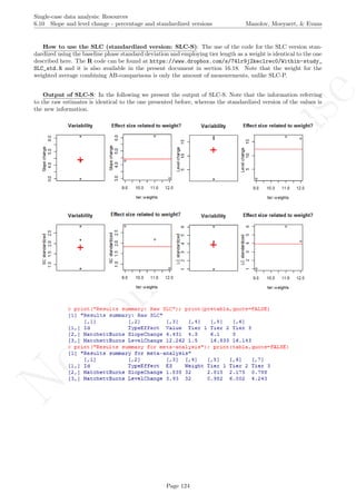
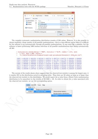
6.10 Slope and level change - percentage and standardized versions Manolov, Moeyaert, & Evans
6.10 Slope and level change - percentage and standardized versions
Name of the technique: Slope and level change - percentage version (SLC-P)
Authors and suggested readings: The SLC-P was proposed by Manolov and Rochat (2015) as an ex-
tension of the Slope and level change procedure (Solanas, Manolov, & Onghena, 2010). The authors offer the
details for this procedure. Moreover, this indicator is applicable to designs that include several AB-comparisons
offering both separate estimates and an overall one. The combination of the individual AB-comparisons is
achieved via a weighted average, in which the weight is directly related to the amount of measurements and
inversely related to the variability of effects (i.e., similar to Hershberger et al.’s [1999] replication effect quan-
tification proposed as a moderator).
Software that can be used: The SLC-P can be implemented via an R code developed by R. Manolov.
How to obtain the software (percentage version): The R code for applying the SLC (percent) at
the within-studies level is available at https://www.dropbox.com/s/o0ukt01bf6h3trs/Within-study_SLC_
percent.R and also in the present document in section 16.17.
After downloading the file, it can easily be manipulated with a text editor such Notepad, apart from more
specific editors like RStudio (http://www.rstudio.com/) or Vim (http://www.vim.org/).
Page 115](https://image.slidesharecdn.com/635a0af9-e378-45de-b512-1e1e88e419b8-160210073243/85/Tutorial-119-320.jpg)


![No
com
m
ercialuse
Single-case data analysis: Resources
10.0 Application of two-level multilevel models for analysing data Manolov, Moeyaert, & Evans
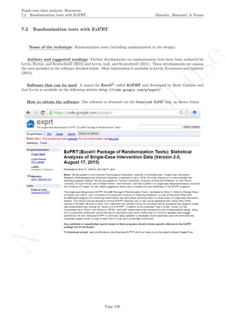
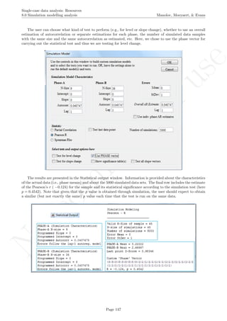
While installing takes place only once for each package, any package should be loaded when each new R
session is started using the option Load package from the menu Packages.
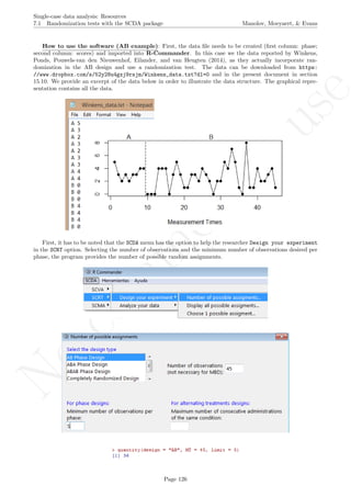
How to use the software: To illustrate the use of the nlme package, we will focus on the data set analysed
by Baek et al. (2014) and published by Jokel, Rochon, and Anderson (2010). This dataset can be downloaded
from https://www.dropbox.com/s/2yla99epxqufnm7/Two-level%20data.txt?dl=0 and is also available in
the present document in section 15.9. For the ones who prefer using the —SAS code for two-level models
detailed information is provided in Moyaert, Ferron, Beretvas, and Van Den Noortgate (2014).
We digitized the data via Plot Digitizer 2.6.3 (http://plotdigitizer.sourceforge.net) focusing only
on the first two phases in each tier. One explanation for the differences in the results obtained here and in
the aforementioned article may be due to the fact that here we use the R package nlme, whereas Baek and
colleagues used SAS proc mixed [SAS Institute Inc., 1998] and Kenward-Roger estimate of degrees of free-
dom (unlike the nlme package). SAS proc mixed potentially handles missing data differently, which can
potentially affect the estimation of autocorrelation). Thus, the equivalence across programs is an issue yet to be
solved and it needs to be kept in mind when results are obtained with different software. Another explanation
for differences in the results may be due to the fact that we digitized the data ourselves, which does not ensure
that that the scores retrieved by Baek et al. (2014) are exactly the same.
Page 155](https://image.slidesharecdn.com/635a0af9-e378-45de-b512-1e1e88e419b8-160210073243/85/Tutorial-159-320.jpg)


![No
com
m
ercialuse
Single-case data analysis: Resources
10.0 Application of two-level multilevel models for analysing data Manolov, Moeyaert, & Evans
Allowing for the treatment effect on trend to vary across lists implies the following reduction: 68.892−9.038
68.892 =
59.854
68.892 86.88%. Allowing for the average treatment effect to vary across lists implies the following reduction:
65.079−9.038
65.079 = 56.041
65.079 86.11%.
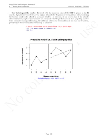
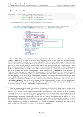
Apart from the numerical results, it is also possible to obtain a graphical representation of the data and of
the model fitted. In the following we present the R code for plotting all data on the same graph, distinguishing
the different cases/tiers with different colours. In order for the code presented below to be used for any dataset,
we now refer to the model as Multilevel.Model instead of Baek.Model and rename the dataset itself from
Jokel to Dataset. We also rename the dependent variable from Percent to the more general Score, as well
as changing List to Case when distinguishing the different cases. Finally, we also continue working only with
the complete rows (i.e., not taking missing data into account).
Multilevel.Model <- Baek.Model
Dataset <- Jokel[complete.cases(Jokel),]
names(Dataset)[names(Dataset)=="Percent"] <- "Score"
names(Dataset)[names(Dataset)=="List"] <- "Case"
From here on, the remaining code can be used by all researchers and is not specific to the dataset used in
the current example. The following two lines of code save the fitted values, according to the model used. The
user has only to change the name of
fit <- fitted(Multilevel.Model)
Dataset <- cbind(Dataset,fit)
The following piece of code is used for assigning colours to the different cases/tiers and it has been created
to handle 3 to 10 cases per study, although it can easily be modified.
tiers <- max(Dataset$Case)
lengths <- c(0,tiers)
for (i in 1:tiers)
lengths[i] <- length(Dataset$Time[Dataset$Case==i])
# Create a vector with the colours to be used
if (tiers == 3) cols <- c("red","green","blue")
if (tiers == 4) cols <- c("red","green","blue","black")
if (tiers == 5) cols <- c("red","green","blue","black",
"grey")
if (tiers == 6) cols <- c("red","green","blue","black",
"grey","orange")
if (tiers == 7) cols <- c("red","green","blue","black",
"grey","orange","violet")
if (tiers == 8) cols <- c("red","green","blue","black",
"grey","orange","violet","yellow")
if (tiers == 9) cols <- c("red","green","blue","black",
"grey","orange","violet","yellow","brown")
if (tiers == 10) cols <- c("red","green","blue","black",
"grey","orange","violet","yellow","brown","pink")
Page 159](https://image.slidesharecdn.com/635a0af9-e378-45de-b512-1e1e88e419b8-160210073243/85/Tutorial-163-320.jpg)
![No
com
m
ercialuse
Single-case data analysis: Resources
10.0 Application of two-level multilevel models for analysing data Manolov, Moeyaert, & Evans
# Create a column with the colors
colors <- rep("col",length(Dataset$Time))
colors[1:lengths[1]] <- cols[1]
sum <- lengths[1]
for (i in 2:tiers)
{
colors[(sum+1):(sum+lengths[i])] <- cols[i]
sum <- sum + lengths[i]
}
Dataset <- cbind(Dataset,colors)
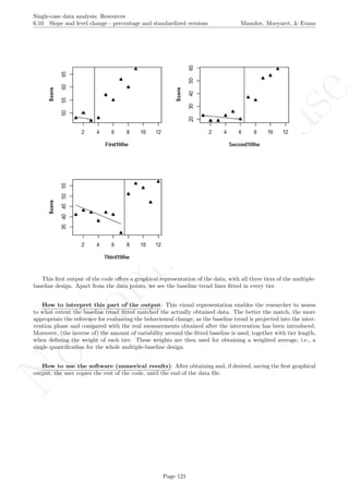
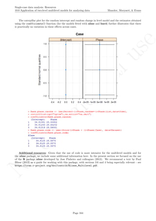
Finally, the numerical values of the coefficients estimated for each case and their graphical representation is
obtained copy-pasting in the R console the following lines of code:
# Print the values of the coefficients estimated
coefficients(Baek.Model)
# Represent the results graphically
plot(Score[Case==1]~Time[Case==1], data=Dataset,
xlab="Time", ylab="Score",
xlim=c(1,max(Dataset$Time)),
ylim=c(min(Dataset$Score),max(Dataset$Score)))
for (i in 1:tiers)
{
points(Score[Case==i]~Time[Case==i], col=cols[i],data=Dataset)
lines(Dataset$Time[Dataset$Case==i],Dataset$fit[Dataset$Case==i],col=cols[i])
}
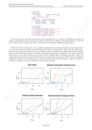
The graph shows the slightly different intercepts and flat (no trend being modelled) baseline levels. More-
over, the different slopes in the intervention phases are made evident. The amount of across-cases variability
Page 160](https://image.slidesharecdn.com/635a0af9-e378-45de-b512-1e1e88e419b8-160210073243/85/Tutorial-164-320.jpg)

![No
com
m
ercialuse
Single-case data analysis: Resources
10.0 Application of two-level multilevel models for analysing data Manolov, Moeyaert, & Evans
install.packages("lattice") # In case the package has not been installed
require(lattice) # Load
qqmath(ranef(Model.lme4, condVar=TRUE), strip=TRUE)$Case
The caterpillar plot shows that there is considerable variability in all three effects around the estimated
averages. Actually, only the intercept and change in level estimates for the second tier are well represented by
the averages, as their confidence intervals include the average estimates across cases. The values represented in
the caterpillar plot can be reconstructed from the results.
Model.lme4
coefficients(Model.lme4)
coefficients(Model.lme4)$Case[,1] - 34.12
coefficients(Model.lme4)$Case[,2] - 40.92
coefficients(Model.lme4)$Case[,3] - 9.39
In case in your version of R, the previous code does not work, you should try:
Model.lme4
fixef(Model.lme4)
ranef(Model.lme4)
Page 162](https://image.slidesharecdn.com/635a0af9-e378-45de-b512-1e1e88e419b8-160210073243/85/Tutorial-166-320.jpg)


![No
com
m
ercialuse
Single-case data analysis: Resources
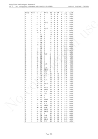
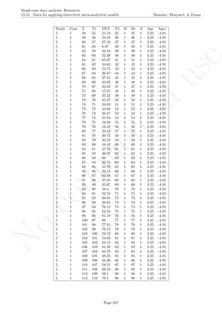
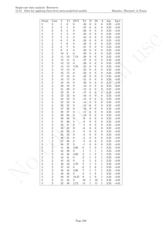
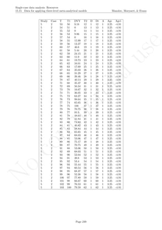
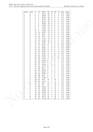
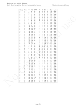
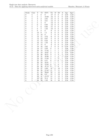
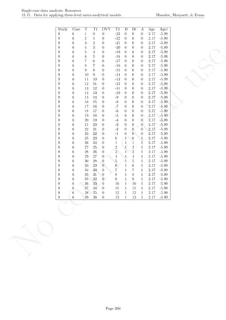
11.3 Application of three-level multilevel models for meta-analysing data Manolov, Moeyaert, & Evans
While installing takes place only once for each package, any package should be loaded when each new R
session is started using the option Load package from the menu Packages.
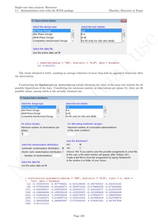
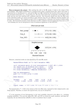
How to use the software& How to interpret the result: To illustrate the use of the nlme package,
we will focus on the data set analysed by Moeyaert, Ferron, Beretvas, and Van Den Noortgate (2014) and pub-
lished by Laski, Charlop, and Schreibman (1988) LeBlanc, Geiger, Sautter, and Sidener (2007), Schreibman,
Stahmer, Barlett, and Dufek (2009), Shrerer and Schreibman (2005), Thorp, Stahmer, and Schreibman (1995),
selecting only the data dealing with appropriate and/or spontaneous speech behaviours. In this case the purpose
is to combine data across several single-case studies and therefore we need to take a three-level structure into
account, that is, measurements are nested within cases and cases in turn are nested within studies. Using the
nlme package, we can take this nested structure into account. In contrast, we previously described the case in
which a two-level model (section ??) is used for analyse the data within a single study.
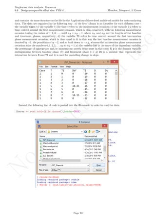
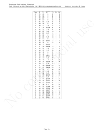
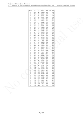
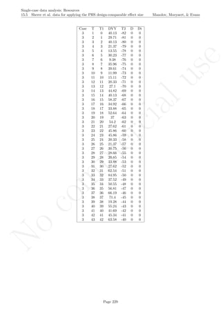
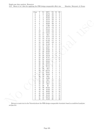
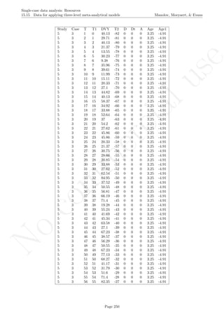
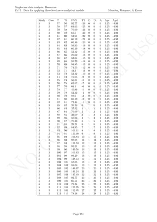
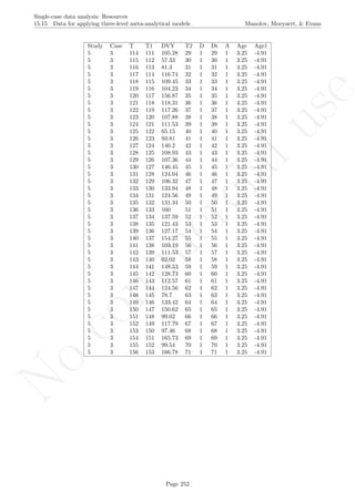
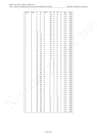
The data are organised in the following way: a) there should be an identified for each different study -
here we used the variable Study in the first column [see an extract of the data table after this explanation];
b) there should also be an identifier for each different case - the variable Case in the second column; c) the
variable T (for time) refers to the measurement occasion; d) the variable T1 refers to time centred around
the first measurement occasion, which is thus equal to 0, with the following measurement occasion taking
the values of 1, 2, 3, ..., until nA + nB − 1, where nA and nB are the lengths of the baseline and treatment
phases, respectively; e) the variable T2 refers to time centred around the first intervention phase measurement
occasion, which is thus equal to 0; in this way the last baseline measurement occasion is denoted by −1,
the penultimate by −2, and so forth down to −nA, whereas the intervention phase measurement occasions
take the numbers 0, 1, 2, 3, ... up to nB − 1; f) the variable DVY is the score of the dependent variable:
the percentage of appropriate and/or spontaneous speech behaviours in this case; g) D is the dummy variable
distinguishing between baseline phase (0) and treatment phase (1); h) Dt is a variable that represents the
interaction between D and T2 and it is used for modelling change in slope; i) Age is a second-level predictor
representing the age of the participants (i.e., the Cases); j) Age1 is the same predictor centred at the average age
of all participants; this centring is performed in order to make the intercept more meaningful, so that it represents
the expected score (percentage of appropriate and/or spontaneous speech behaviours) for the average-aged
individual rather than for individuals with age equal to zero, which would be less meaningful. The dataset can
be downloaded from https://www.dropbox.com/s/e2u3edykupt8nzi/Three-level%20data.txt?dl=0 and in
the present document in section 15.15.
Page 182](https://image.slidesharecdn.com/635a0af9-e378-45de-b512-1e1e88e419b8-160210073243/85/Tutorial-186-320.jpg)


![No
com
m
ercialuse
Single-case data analysis: Resources
12.0 References Manolov, Moeyaert, & Evans
single-case designs. Journal of School Psychology, 52, 213-230.
Swaminathan, H., Rogers, H. J., Horner, R., Sugai, G., & Smolkowski, K. (2014). Regression models for the
analysis of single case designs. Neuropsychological Rehabilitation, 24, 554-571.
Thorp, D. M., Stahmer, A. C., & Schreibman, L. (1995). The effects of sociodramatic play training on
children with autism. Journal of Autism and Developmental Disorders, 25, 265-282.
Tukey, J. W. (1977). Exploratory data analysis. London, UK: Addison-Wesley.
Vannest, K. J., Parker, R. I., & Gonen, O. (2011). Single Case Research: web based calculators for SCR
analysis. (Version 1.0) [Web-based application]. College Station, TX: Texas A&M University. Retrieved Friday
12th July 2013. Available from singlecaseresearch.org
Van Den Noortgate, W., & Onghena, P. (2003). Hierarchical linear models for the quantitative integration
of effect sizes in single-case research. Behavior Research Methods, Instruments, & Computers, 35, 1-10.
Van den Noortgate, W., & Onghena, P. (2008). A multilevel meta-analysis of single-subject experimental
design studies. Evidence Based Communication Assessment and Intervention, 2, 142-151.
Wehmeyer, M. L., Palmer, S. B., Smith, S. J., Parent, W., Davies, D. K., & Stock, S. (2006). Technology use
by people with intellectual and developmental disabilities to support employment activities: A single-subject
design meta-analysis. Journal of Vocational Rehabilitation, 24, 81-86.
Wendt, O. (2009). Calculating effect sizes for single-subject experimental designs: An overview and compari-
son. Paper presented at The Ninth Annual Campbell Collaboration Colloquium, Oslo, Norway. Retrieved June
29, 2015 from http://www.campbellcollaboration.org/artman2/uploads/1/Wendt_calculating_effect_
sizes.pdf
Winkens, I., Ponds, R., Pouwels-van den Nieuwenhof, C., Eilander, H., & van Heugten, C. (2014). Using
single-case experimental design methodology to evaluate the effects of the ABC method for nursing staff on
verbal aggressive behaviour after acquired brain injury. Neuropsychological Rehabilitation, 24, 349-364.
Wolery, M., Busick, M., Reichow, B., & Barton, E. E. (2010). Comparison of overlap methods for quantita-
tively synthesizing single-subject data. Journal of Special Education, 44, 18-29.
Page 201](https://image.slidesharecdn.com/635a0af9-e378-45de-b512-1e1e88e419b8-160210073243/85/Tutorial-205-320.jpg)


![No
com
m
ercialuse
Single-case data analysis: Resources
13.0 Appendix A: Some additional information about R Manolov, Moeyaert, & Evans
First, see an example of how different types of arrays (i.e., vectors, two- and three-dimensional matrices) are
defined:
# Assign values to an array: one-dimensional vector
v <- array(c(1,2,3,4,5,6),dim=c(6))
v
## [1] 1 2 3 4 5 6
# Assign values to an array: two-dimensional matrix
m <- array(c(1,2,3,4,5,6),dim=c(2,4))
m
## [,1] [,2] [,3] [,4]
## [1,] 1 3 5 1
## [2,] 2 4 6 2
# Assign values to an array: three-dimensional array
a <- array(c(1,2,3,4,5,6,7,8),dim=c(2,1,3))
a
## , , 1
##
## [,1]
## [1,] 1
## [2,] 2
##
## , , 2
##
## [,1]
## [1,] 3
## [2,] 4
##
## , , 3
##
## [,1]
## [1,] 5
## [2,] 6
Operations can be carried out with the whole vector (e.g., adding 1 to all values) or with different parts of a
vector. These different segments are selected according to the positions that the values have within the vector.
For instance, the second value in the vector x is 7, whereas the segment containing the first and second values
consists of the scalars 2 and 7.
# Create a vector
x <- c(1,6,9)
# Add a constant to all values in the vector
x <- x + 1
x
## [1] 2 7 10
# A scalar within the vector
x[2]
## [1] 7
# A subvector within the vector
x[1:2]
## [1] 2 7
Page 204](https://image.slidesharecdn.com/635a0af9-e378-45de-b512-1e1e88e419b8-160210073243/85/Tutorial-208-320.jpg)
![No
com
m
ercialuse
Single-case data analysis: Resources
13.0 Appendix A: Some additional information about R Manolov, Moeyaert, & Evans
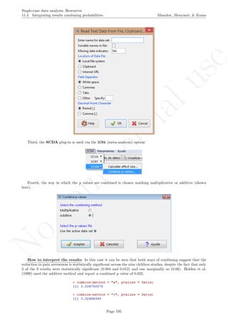
Regarding data input, in R it is possible to open and read a data file (using the function read.table) or to
enter the data manually, creating a data.frame (called here “data1”) consisting of several variables (here only
two: ”studies” and ”grades”). It is possible to work with one of the variables of the data frame or even with a
single value of a variable.
# Manual entry
studies <- c("Humanities", "Humanities", "Sciences", "Sciences")
grades <- c(5,9,7,7)
data1 <- data.frame(studies,grades)
data1
## studies grades
## 1 Humanities 5
## 2 Humanities 9
## 3 Sciences 7
## 4 Sciences 7
# Read an already created data file
data2 <- read.table("C:/Users/WorkStation/Dropbox/data2.txt",header=TRUE)
data2
## studies grades
## 1 Humanities 5
## 2 Humanities 9
## 3 Sciences 7
## 4 Sciences 7
# Refer to one variable within the data set using £
data1$grades
## [1] 5 9 7 7
# Refer to one variable within the data set, when its location is known
data1[2,2]
## [1] 9
Regarding, some of the most useful aspects of programming (loops and conditional statements), an example
is provided below. The code provided computes the average grade for students that have studied Humanities
only (mean h), by first computing the sum h and then dividing it by ppts h (the number of students from this
are). For iteration or looping, the internal function for() is used for reading all the grades, although other
options from the apply family can also be used. For selecting only students of Humanities the conditional
function if() is used.
# Set the counters to zero
sum_h <- 0
ppts_h <- 0
for (i in 1:length(data1$studies))
if(data1$studies[i]=="Humanities")
{
sum_h <- sum_h + data1$grades[i]
ppts_h <- ppts_h + 1
}
#Obtain the mean on the basis of the sum and the number of values (participants)
sum_h
## [1] 14
ppts_h
## [1] 2
Page 205](https://image.slidesharecdn.com/635a0af9-e378-45de-b512-1e1e88e419b8-160210073243/85/Tutorial-209-320.jpg)
![No
com
m
ercialuse
Single-case data analysis: Resources
13.0 Appendix A: Some additional information about R Manolov, Moeyaert, & Evans
mean_h <- sum_h/ppts_h
mean_h
## [1] 7
Regarding user-created functions, below is provided information on how to use a function called “moda”
yielding the modal value of a variable. Such a function needs to be available in the workspace, that is, pasted
into the R console before calling it. Calling itself requires using the function name and the arguments in
parenthesis needed for the function to operate with (here: the array including the values of the variable).
# Enter the data
data3 <- c(1,2,2,3)
# Define the function: this makes it availabe in the workspace
moda <- function(X){
if (is.numeric(X))
moda <- as.numeric(names(table(X))[which(table(X)==max(table(X)))]) else
moda <- names(table(X))[which(table(X)==max(table(X)))]
list(moda=moda,frequency.table=table(X))
}
# Call the user-defined function using the name of the vector with the data
moda(data3)
## $moda
## [1] 2
##
## $frequency.table
## X
## 1 2 3
## 1 2 1
The second example of calling user-defined functions refers to a function called V.Cramer and yielding
a quantification (in terms of Cram´er’s V ) of the strength of relation between to categorical variables. The
arguments required when calling the function are, therefore, two arrays containing the categories of the variables.
# Enter the data
studies <- c("Sciences", "Sciences", "Humanities", "Humanities")
FinalGrades <- c("Excellent", "Excellent", "Excellent", "Very good")
# Define the function: this makes it availabe in the workspace
V.Cramer <- function(X,Y){
tabla <- xtabs(~X+Y)
Cramer <- sqrt(as.numeric(chisq.test(tabla,correct=FALSE)$statistic/
(sum(tabla)*min(dim(tabla)-1))) )
return(V.Cramer=Cramer)
}
# Call the user-defined function using the name of the vector with the data
V.Cramer(studies,FinalGrades)
## [1] 0.5773503
Page 206](https://image.slidesharecdn.com/635a0af9-e378-45de-b512-1e1e88e419b8-160210073243/85/Tutorial-210-320.jpg)


![No
com
m
ercialuse
Single-case data analysis: Resources
16.2 Standard deviation bands Manolov, Moeyaert, & Evans
16.2 Standard deviation bands
After inputting the data actually obtained, the rest of the code is only copied and pasted.
# Input data: values in () separated by commas
# n_a denotes number of baseline phase measurements
score <- c(4,7,5,6,8,10,9,7,9)
n_a <- 4
# Input the standard deviations' rule for creating the bands
SD_value <- 2
# Copy and paste the rest of the code in the R console
# Objects needed for the calculations
size <- length(score)
phaseA <- score[1:n_a]
phaseB <- score[(n_a+1):nsize]
mean_A <- rep(mean(phaseA),n_a)
# Construct bands
band <- sd(phaseA)*SD_value
upper_band <- mean(phaseA) + band
lower_band <- mean(phaseA) - band
# As vectors
upper <- rep(upper_band,nsize)
lower <- rep(lower_band,nsize)
# Counters
count_out_up <- 0
count_out_low <- 0
consec_out_up <- 0
consec_out_low <- 0
greatest_low <- 0
greatest_up <- 0
# Count
for (i in 1:length(phaseB))
{
# Count below
if (phaseB[i] < lower[n_a+i])
{ count_out_low <- count_out_low + 1;
consec_out_low <- consec_out_low + 1} else
{ if(greatest_low < consec_out_low) greatest_low <-
+ consec_out_low;
consec_out_low <- 0; }
if (greatest_low < consec_out_low) greatest_low <-
+ consec_out_low
# Count above
if (phaseB[i] > upper[n_a+i])
{ count_out_up <- count_out_up + 1;
Page 270](https://image.slidesharecdn.com/635a0af9-e378-45de-b512-1e1e88e419b8-160210073243/85/Tutorial-274-320.jpg)
![No
com
m
ercialuse
Single-case data analysis: Resources
16.2 Standard deviation bands Manolov, Moeyaert, & Evans
consec_out_up <- consec_out_up + 1} else
{ if(greatest_up < consec_out_up) greatest_up <-
+ consec_out_up;
consec_out_up <- 0}
if (greatest_up < consec_out_up) greatest_up <-
+ consec_out_up
}
#############################
# Construct the plot with the SD bands
indep <- 1:nsize
# Plot limits
minimal <- min(min(score),min(lower))
maximal <- max(max(score),max(upper))
# Plot data
plot(indep,score, xlim=c(indep[1],indep[length(indep)]),
ylim=c((minimal-1),(maximal+1)), xlab="Measurement time",
ylab="Score", font.lab=2)
lines(indep[1:n_a],score[1:n_a])
lines(indep[(n_a+1):nsize],score[(n_a+1):nsize])
abline (v=(n_a+0.5))
points(indep, score, pch=24, bg="black")
title(main="Standard deviation bands")
# Phase A mean & projections with SD-bands
lines(indep[1:n_a],mean_A)
lines(indep,upper,type="b")
lines(indep,lower,type="b")
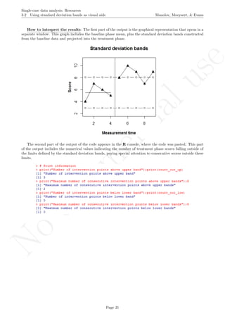
# Print information
print("Number of intervention points above upper band");
print(count_out_up)
print("Maximum number of consecutive intervention points
above upper bands");
print(greatest_up)
print("Number of intervention points below lower band");
print(count_out_low)
print("Maximum number of consecutive intervention points
below lower bands");
print(greatest_low)
Page 271](https://image.slidesharecdn.com/635a0af9-e378-45de-b512-1e1e88e419b8-160210073243/85/Tutorial-275-320.jpg)
![No
com
m
ercialuse
Single-case data analysis: Resources
16.2 Standard deviation bands Manolov, Moeyaert, & Evans
Code ends here. Default output of the code below:
2 4 6 8
246810
Measurement time
Score
Standard deviation bands
## [1] "Number of intervention points above upper band"
## [1] 3
## [1] "Maximum number of consecutive intervention points n above upper bands"
## [1] 2
## [1] "Number of intervention points below lower band"
## [1] 0
## [1] "Maximum number of consecutive intervention points n below lower bands"
## [1] 0
Return to main text in the Tutorial about the Standard deviations band: section 3.2.
Page 272](https://image.slidesharecdn.com/635a0af9-e378-45de-b512-1e1e88e419b8-160210073243/85/Tutorial-276-320.jpg)
![No
com
m
ercialuse
Single-case data analysis: Resources
16.3 Estimating and projecting baseline trend Manolov, Moeyaert, & Evans
16.3 Estimating and projecting baseline trend
After inputting the data actually obtained and specifying the rules for constructing the intervals, the rest of
the code is only copied and pasted.
# Input data: values in () separated by commas
# n_a denotes number of baseline phase measurements
score <- c(1,3,5,5,10,8,11,14)
n_a <- 4
# Input the % of the Median to use for constructing the envelope
md_percentage <- 20
# Input the interquartile range to use for constructing the envelope
IQR_value <- 1.5
# Choose figures' display
display<- 'vertical' # Alternatively 'horizontal'
# Copy and paste the rest of the code in the R console
# Objects needed for the calculations
md_addsub <- md_percentage/200
nsize <- length(score)
indep <- 1:nsize
# Construct phase vectors
a1 <- score[1:n_a]
b1 <- score[(n_a+1):nsize]
##############################
# Split-middle method
# Divide the phase into two parts of equal size:
# even number of measuments
if (length(a1)%%2==0)
{
part1 <- 1:(length(a1)/2)
part1 <- a1[1:(length(a1)/2)]
part2 <- ((length(a1)/2)+1):length(a1)
part2 <- a1[((length(a1)/2)+1):length(a1)]
}
# Divide the phase into two parts of equal size:
# odd number of measurements
Page 273](https://image.slidesharecdn.com/635a0af9-e378-45de-b512-1e1e88e419b8-160210073243/85/Tutorial-277-320.jpg)
![No
com
m
ercialuse
Single-case data analysis: Resources
16.3 Estimating and projecting baseline trend Manolov, Moeyaert, & Evans
if (length(a1)%%2==1)
{
part1 <- 1:((length(a1)-1)/2)
part1 <- a1[1:((length(a1)-1)/2)]
part2 <- (((length(a1)+1)/2)+1):length(a1)
part2 <- a1[(((length(a1)+1)/2)+1):length(a1)]
}
# Obtain the median in each section
median1 <- median(part1)
median2 <- median(part2)
# Obtain the midpoint in each section
midp1 <- (length(part1)+1)/2
if (length(a1)%%2==0) midp2 <- length(part1) + (length(part2)+1)/2
if (length(a1)%%2==1) midp2 <- length(part1) + 1 + (length(part2)+1)/2
# Obtain the values of the split-middle trend: "regla de 3"
slope <- (median2-median1)/(midp2-midp1)
sm.trend <- 1:length(a1)
# Whole number function
is.wholenumber <-
function(x, tol = .Machine$double.eps^0.5)
+ abs(x - round(x)) < tol
if (!is.wholenumber(midp1))
{
sm.trend[midp1-0.5] <- median1 - (slope/2)
for (i in 1:length(part1))
if ((midp1-0.5 - i) >= 1) sm.trend[(midp1-0.5 - i)] <-
+ sm.trend[(midp1-0.5-i + 1)] - slope
for (i in (midp1+0.5):length(sm.trend))
sm.trend[i] <- sm.trend[i-1] + slope
}
if (is.wholenumber(midp1))
{
sm.trend[midp1] <- median1
for (i in 1:length(part1))
if ((midp1 - i) >= 1) sm.trend[(midp1 - i)] <-
+ sm.trend[(midp1-i + 1)] - slope
for (i in (midp1+1):length(sm.trend))
sm.trend[i] <- sm.trend[i-1] + slope
}
# Consutructing envelopes
# Construct envelope 20% median (Gast & Spriggs, 2010)
envelope <- median(a1)*md_addsub
upper_env <- 1:length(a1)
upper_env <- sm.trend + envelope
lower_env <- 1:length(a1)
lower_env <- sm.trend - envelope
# Construct envelope 1.5 IQR (add to median)
tukey.eda <- IQR_value*IQR(a1)
upper_IQR <- 1:length(a1)
Page 274](https://image.slidesharecdn.com/635a0af9-e378-45de-b512-1e1e88e419b8-160210073243/85/Tutorial-278-320.jpg)
![No
com
m
ercialuse
Single-case data analysis: Resources
16.3 Estimating and projecting baseline trend Manolov, Moeyaert, & Evans
upper_IQR <- sm.trend + tukey.eda
lower_IQR <- 1:length(a1)
lower_IQR <- sm.trend - tukey.eda
# Project split middle trend and envelope
projected <- 1:length(b1)
proj_env_U <- 1:length(b1)
proj_env_L <- 1:length(b1)
proj_IQR_U <- 1:length(b1)
proj_IQR_L <- 1:length(b1)
projected[1] <- sm.trend[length(sm.trend)]+slope
proj_env_U[1] <- upper_env[length(upper_env)]+slope
proj_env_L[1] <- lower_env[length(lower_env)]+slope
proj_IQR_U[1] <- upper_IQR[length(upper_IQR)]+slope
proj_IQR_L[1] <- lower_IQR[length(lower_IQR)]+slope
for (i in 2:length(b1))
{
projected[i] <- projected[i-1]+slope
proj_env_U[i] <- proj_env_U[i-1]+slope
proj_env_L[i] <- proj_env_L[i-1]+slope
proj_IQR_U[i] <- proj_IQR_U[i-1]+slope
proj_IQR_L[i] <- proj_IQR_L[i-1]+slope
}
# Count the number of values within the envelope
in_env <-0
in_IQR <- 0
for (i in 1:length(b1))
{
if ( (b1[i] >= proj_env_L[i]) && (b1[i] <= proj_env_U[i]) )
in_env <- in_env + 1
if ( (b1[i] >= proj_IQR_L[i]) && (b1[i] <= proj_IQR_U[i]) )
in_IQR <- in_IQR + 1
}
prop_env <- in_env/length(b1)
prop_IQR <- in_IQR/length(b1)
##############################
# Construct the plot with the median-based envelope
if (display=="vertical") {rows <- 2; cols <- 1} else
+ {rows <- 1; cols <- 2}
minimal1 <- min(min(score),min(proj_env_L))
maximal1 <- max(max(score),max(proj_env_U))
par(mfrow=c(rows,cols))
# Plot data
plot(indep,score, xlim=c(indep[1],indep[length(indep)]),
ylim=c((minimal1-1),(maximal1+1)), xlab="Measurement time",
ylab="Score", font.lab=2)
lines(indep[1:n_a],score[1:n_a])
Page 275](https://image.slidesharecdn.com/635a0af9-e378-45de-b512-1e1e88e419b8-160210073243/85/Tutorial-279-320.jpg)
![No
com
m
ercialuse
Single-case data analysis: Resources
16.3 Estimating and projecting baseline trend Manolov, Moeyaert, & Evans
lines(indep[(n_a+1):nsize],score[(n_a+1):nsize])
abline (v=(n_a+0.5))
points(indep, score, pch=24, bg="black")
title(main="Md-based envelope around projected SM trend")
# Split-middle trend & projections with limits
lines(indep[1:n_a],sm.trend[1:n_a])
lines(indep[(n_a+1):nsize],proj_env_U,type="b")
lines(indep[(n_a+1):nsize],proj_env_L,type="b")
# Construct the plot with the IQR-based envelope
minimal2 <- min(min(score),min(proj_IQR_L))
maximal2 <- max(max(score),max(proj_IQR_U))
# Plot data
plot(indep,score, xlim=c(indep[1],indep[length(indep)]),
ylim=c((minimal2-1),(maximal2+1)), xlab="Measurement time",
ylab="Score", font.lab=2)
lines(indep[1:n_a],score[1:n_a])
lines(indep[(n_a+1):nsize],score[(n_a+1):nsize])
abline (v=(n_a+0.5))
points(indep, score, pch=24, bg="black")
title(main="IQR-based envelope around projected SM trend")
# Split-middle trend & projections with limits
lines(indep[1:n_a],sm.trend[1:n_a])
lines(indep[(n_a+1):nsize],proj_IQR_U,type="b")
lines(indep[(n_a+1):nsize],proj_IQR_L,type="b")
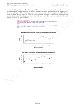
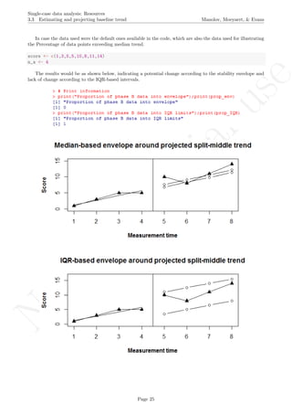
# Print information
print("Proportion of phase B data into envelope");
print(prop_env)
print("Proportion of phase B data into IQR limits");
print(prop_IQR)
Page 276](https://image.slidesharecdn.com/635a0af9-e378-45de-b512-1e1e88e419b8-160210073243/85/Tutorial-280-320.jpg)
![No
com
m
ercialuse
Single-case data analysis: Resources
16.3 Estimating and projecting baseline trend Manolov, Moeyaert, & Evans
Code ends here. Default output of the code below:
1 2 3 4 5 6 7 8
051015
Measurement time
Score
Median−based envelope around projected split−middle trend
1 2 3 4 5 6 7 8
051015
Measurement time
Score
IQR−based envelope around projected split−middle trend
## [1] "Proportion of phase B data into envelope"
## [1] 0
## [1] "Proportion of phase B data into IQR limits"
## [1] 1
Return to main text in the Tutorial about Projecting trend:section 3.3.
Page 277](https://image.slidesharecdn.com/635a0af9-e378-45de-b512-1e1e88e419b8-160210073243/85/Tutorial-281-320.jpg)
![No
com
m
ercialuse
Single-case data analysis: Resources
16.4 Graph rotation for controlling for baseline trend Manolov, Moeyaert, & Evans
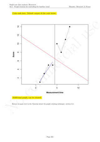
16.4 Graph rotation for controlling for baseline trend
After inputting the data actually obtained, the rest of the code is only copied and pasted.
This code requires that the rgl package for R (which it loads). In case it has not been previously installed,
this is achieved in the R console via the following code:
install.packages('rgl')
Once the package is installed, the rest of the code is used, as follows:
# Input data: values in () separated by commas
# n_a denotes number of baseline phase measurements
score <- c(1,3,5,5,10,8,11,14)
n_a <- 4
# Copy and paste the rest of the code in the R console
nsize <- length(score)
tiempo <- 1:nsize
# Construct phase vectors
a1 <- score[1:n_a]
b1 <- score[(n_a+1):nsize]
if (n_a%%3==0)
{
tiempoA <- 1:n_a
corte1 <- quantile(tiempoA,0.33)
corte2 <- quantile(tiempoA,0.66)
final1 <- trunc(corte1)
final2 <- trunc(corte2)
part1.md <- median(score[1:final1])
length.p1 <- final1
times1 <- 1:final1
midp1 <- median(times1)
part2.md <- median(score[(final1+1):final2])
times2 <- (final1+1):final2
midp2 <- median(times2)
part3.md <- median(score[(final2+1):n_a])
times3 <- (final2+1):n_a
midp3 <- median(times3)
}
if (n_a%%3==1)
{
tiempoA <- 1:n_a
corte1 <- quantile(tiempoA,0.33)
corte2 <- quantile(tiempoA,0.66)
final1 <- trunc(corte1)
final2 <- trunc(corte2)
part1.md <- median(score[1:(final1+1)])
length.p1 <- final1+1
Page 278](https://image.slidesharecdn.com/635a0af9-e378-45de-b512-1e1e88e419b8-160210073243/85/Tutorial-282-320.jpg)
![No
com
m
ercialuse
Single-case data analysis: Resources
16.4 Graph rotation for controlling for baseline trend Manolov, Moeyaert, & Evans
times1 <- 1:(final1+1)
midp1 <- median(times1)
part2.md <- median(score[(final1+1):(final2+1)])
times2 <- (final1+1):(final2+1)
midp2 <- median(times2)
part3.md <- median(score[(final2+1):n_a])
times3 <- (final2+1):n_a
midp3 <- median(times3)
}
if (n_a%%3==2)
{
tiempoA <- 1:n_a
corte1 <- quantile(tiempoA,0.33)
corte2 <- quantile(tiempoA,0.66)
final1 <- trunc(corte1)
final2 <- trunc(corte2)
part1.md <- median(score[1:final1])
length.p1 <- final1
times1 <- 1:final1
midp1 <- median(times1)
part2.md <- median(score[(final1+1):final2])
times2 <- (final1+1):final2
midp2 <- median(times2)
part3.md <- median(score[(final2+1):n_a])
times3 <- (final2+1):n_a
midp3 <- median(times3)
}
# Obtain the values of the split-middle trend: "regla de 3"
slope <- (part3.md-part1.md)/(midp3-midp1)
sm.trend <- 1:length(a1)
# Whole number function
is.wholenumber <-
function(x, tol = .Machine$double.eps^0.5)
+ abs(x - round(x)) < tol
if (!is.wholenumber(midp1))
{
sm.trend[midp1-0.5] <- part1.md - (slope/2)
for (i in 1:length.p1)
if ((midp1-0.5 - i) >= 1) sm.trend[(midp1-0.5 - i)] <-
+ sm.trend[(midp1-0.5-i + 1)] - slope
for (i in (midp1+0.5):length(sm.trend))
sm.trend[i] <- sm.trend[i-1] + slope
}
if (is.wholenumber(midp1))
{
sm.trend[midp1] <- part1.md
for (i in 1:length.p1)
if ((midp1 - i) >= 1) sm.trend[(midp1 - i)] <-
+ sm.trend[(midp1-i + 1)] - slope
for (i in (midp1+1):length(sm.trend))
sm.trend[i] <- sm.trend[i-1] + slope
}
# Using the middle part: shifting the trend line
Page 279](https://image.slidesharecdn.com/635a0af9-e378-45de-b512-1e1e88e419b8-160210073243/85/Tutorial-283-320.jpg)
![No
com
m
ercialuse
Single-case data analysis: Resources
16.4 Graph rotation for controlling for baseline trend Manolov, Moeyaert, & Evans
sm.trend.shifted <- 1:length(a1)
midX <- midp2
midY <- part2.md
if (is.wholenumber(midX))
{
sm.trend.shifted[midX] <- midY
for (i in (midX-1):1) sm.trend.shifted[i] <-
+ sm.trend.shifted[i+1] - slope
for (i in (midX+1):n_a) sm.trend.shifted[i] <-
+ sm.trend.shifted[i-1] + slope
}
if (!is.wholenumber(midX))
{
sm.trend.shifted[midX-0.5] <- midY-(0.5*slope)
sm.trend.shifted[midX+0.5] <- midY+(0.5*slope)
for (i in (midX-1.5):1) sm.trend.shifted[i] <-
+ sm.trend.shifted[i+1] - slope
for (i in (midX+1.5):n_a) sm.trend.shifted[i] <-
+ sm.trend.shifted[i-1] + slope
}
# Choosing which trend line to use: shifted or not
# according to which one is closer to 50-50 split
if ( abs(sum(a1 < sm.trend)/n_a - 0.5) <=
+ abs(sum(a1 < sm.trend.shifted)/n_a) )
fitted <- sm.trend
if ( abs(sum(a1 < sm.trend)/n_a - 0.5) >
+ abs(sum(a1 < sm.trend.shifted)/n_a) )
fitted <- sm.trend.shifted
# Project split middle trend
sm.trendB <- rep(0,length(b1))
sm.trendB[1] <- fitted[n_a] + slope
for (i in 2:length(b1))
sm.trendB[i] <- sm.trendB[i-1] + slope
##################################################
# Plot data
plot(tiempo,score, xlim=c(tiempo[1],tiempo[nsize]),
xlab="Measurement time", ylab="Score", font.lab=2,asp=TRUE)
lines(tiempo[1:n_a],score[1:n_a],lty=2)
lines(tiempo[(n_a+1):nsize],score[(n_a+1):nsize],lty=2)
abline (v=(n_a+0.5))
points(tiempo, score, pch=24, bg="black")
# Split-middle trend & projections with limits
lines(tiempo[1:n_a],sm.trend, col="blue")
lines(tiempo[(n_a+1):nsize],sm.trendB, col="blue",
lty="dotted")
interv.pt <- sm.trend[n_a] + slope/2
newslope <- (-1/slope)
y1 <- fitted[1]
x1 <- 1
y2 <- fitted[n_a]
x2 <- n_a
y3 <- interv.pt
Page 280](https://image.slidesharecdn.com/635a0af9-e378-45de-b512-1e1e88e419b8-160210073243/85/Tutorial-284-320.jpg)
![No
com
m
ercialuse
Single-case data analysis: Resources
16.4 Graph rotation for controlling for baseline trend Manolov, Moeyaert, & Evans
x3 <- n_a + 0.5
m <- (y1-y2)/(x1-x2)
if (slope!=0) newslope <- (-1/m) else newslope <- 0
ycut <- -(newslope)*x3 + y3
if (slope!=0) abline(a=ycut,b=newslope, col="red") else
abline(v=n_a+0.5,col="red")
linex <- rep(0,n_a+1)
linex[1] <- n_a+0.5
linex[2:(n_a+1)] <- n_a:1
liney <- rep(0,n_a+1)
liney[1] <- interv.pt
liney[2] <- liney[1] - (newslope/2)
for (i in 3:(n_a+1))
liney[i] <- liney[i-1]-newslope
# Rotating the figure with the "rgl" pacakge
library(rgl)
depth <- rep(0,length(score))
plot3d(x=tiempo, y=score,z=depth,xlab="Measurement occasion",
zlab="0", ylab="Score",size=6, asp="iso")
lines3d(x=tiempo[1:n_a],y=score[1:n_a],z=0,lty=2)
lines3d(x=tiempo[(n_a+1):nsize],y=score[(n_a+1):nsize],z=0,lty=2)
lines3d(x=n_a+0.5, y=min(score):max(score),z=0)
if (slope!=0) lines3d(x=linex, y=liney,z=0, col="red") else
lines3d(x=n_a+0.5, y=min(score):max(score),z=0,col="red")
lines3d(x=tiempo[1:n_a],y=sm.trend, z=0, col="blue")
lines3d(x=tiempo[(n_a+1):nsize],y=sm.trendB, z=0, col="blue")
Page 281](https://image.slidesharecdn.com/635a0af9-e378-45de-b512-1e1e88e419b8-160210073243/85/Tutorial-285-320.jpg)
![No
com
m
ercialuse
Single-case data analysis: Resources
16.5 Pairwise data overlap Manolov, Moeyaert, & Evans
16.5 Pairwise data overlap
After inputting the data actually obtained and specifying the aim of the intervention with respect to the target
behavior, the rest of the code is only copied and pasted.
# Input data: values in () separated by commas
# n_a denotes number of baseline phase measurements
score <- c(5,6,7,5,5,7,7,6,8,9,7)
n_a <- 5
# Specify whether the aim is to increase or reduce the behavior
aim<- 'increase' # Alternatively 'reduce'
# Copy and paste the rest of the code in the R console
# Data manipulations
n_b <- length(score)-n_a
phaseA <- score[1:n_a]
phaseB <- score[(n_a+1):length(score)]
nsize <- length(score)
# Compute overlaps
complete <- 0
half <- 0
if (aim == "increase")
{
for (iter1 in 1:n_a)
for (iter2 in 1:n_b)
{if (phaseA[iter1] > phaseB[iter2]) complete <- complete + 1;
if (phaseA[iter1] == phaseB[iter2]) half <- half + 1}
}
if (aim == "reduce")
{
for (iter1 in 1:n_a)
for (iter2 in 1:n_b)
{if (phaseA[iter1] < phaseB[iter2]) complete <- complete + 1;
if (phaseA[iter1] == phaseB[iter2]) half <- half + 1}
}
comparisons <- n_a*n_b
pdo2 <- (complete/comparisons)**2
# Plot data
indep <- 1:length(score)
plot(indep,score, xlim=c(indep[1],indep[length(indep)]),
xlab="Measurement time", ylab="Score", font.lab=2)
abline (v=(n_a+0.5))
points(indep, score, pch=24, bg="black")
lines(indep[1:n_a],score[1:n_a],lty=2)
lines(indep[(n_a+1):nsize],score[(n_a+1):nsize],lty=2)
Page 283](https://image.slidesharecdn.com/635a0af9-e378-45de-b512-1e1e88e419b8-160210073243/85/Tutorial-287-320.jpg)
![No
com
m
ercialuse
Single-case data analysis: Resources
16.5 Pairwise data overlap Manolov, Moeyaert, & Evans
title(main="Pairwise data overlap")
# Line marking the minimal intervention phase measurement
if (aim == "increase")
{
lineA <- rep(max(phaseA),n_a)
lineB <- rep(min(phaseB),n_b)
}
if (aim == "reduce")
{
lineA <- rep(min(phaseA),n_a)
lineB <- rep(max(phaseB),n_b)
}
# Add lines
lines(indep[1:n_a],lineA)
lines(indep[(n_a+1):length(score)],lineB)
# Print result
print("Pairwise data overlap"); print(pdo2)
Page 284](https://image.slidesharecdn.com/635a0af9-e378-45de-b512-1e1e88e419b8-160210073243/85/Tutorial-288-320.jpg)
![No
com
m
ercialuse
Single-case data analysis: Resources
16.5 Pairwise data overlap Manolov, Moeyaert, & Evans
Code ends here. Default output of the code below:
2 4 6 8 10
56789
Measurement time
Score
Pairwise data overlap
## [1] "Pairwise data overlap"
## [1] 0.001111111
Return to main text in the Tutorial about the Pairwise data overlap: section 4.3.
Page 285](https://image.slidesharecdn.com/635a0af9-e378-45de-b512-1e1e88e419b8-160210073243/85/Tutorial-289-320.jpg)
![No
com
m
ercialuse
Single-case data analysis: Resources
16.6 Percentage of data points exceeding median trend Manolov, Moeyaert, & Evans
16.6 Percentage of data points exceeding median trend
After inputting the data actually obtained and specifying the aim of the intervention with respect to the target
behavior, the rest of the code is only copied and pasted.
# Input data: values in () separated by commas
# n_a denotes number of baseline phase measurements
score <- c(1,3,5,5,10,8,11,14)
n_a <- 4
# Specify whether the aim is to increase or reduce the behavior
aim<- 'increase' # Alternatively 'reduce'
# Copy and paste the rest of the code in the R console
# Objects needed for the calculations
nsize <- length(score)
indep <- 1:nsize
# Construct phase vectors
a1 <- score[1:n_a]
b1 <- score[(n_a+1):nsize]
##############################
# Split-middle method
# Divide the phase into two parts of equal size:
# even number of measm
if (length(a1)%%2==0)
{
part1 <- 1:(length(a1)/2)
part1 <- a1[1:(length(a1)/2)]
part2 <- ((length(a1)/2)+1):length(a1)
part2 <- a1[((length(a1)/2)+1):length(a1)]
}
# Divide the phase into two parts of equal size:
# odd number of measm
if (length(a1)%%2==1)
{
part1 <- 1:((length(a1)-1)/2)
part1 <- a1[1:((length(a1)-1)/2)]
part2 <- (((length(a1)+1)/2)+1):length(a1)
part2 <- a1[(((length(a1)+1)/2)+1):length(a1)]
}
# Obtain the median in each section
median1 <- median(part1)
median2 <- median(part2)
Page 286](https://image.slidesharecdn.com/635a0af9-e378-45de-b512-1e1e88e419b8-160210073243/85/Tutorial-290-320.jpg)
![No
com
m
ercialuse
Single-case data analysis: Resources
16.6 Percentage of data points exceeding median trend Manolov, Moeyaert, & Evans
# Obtain the midpoint in each section
midp1 <- (length(part1)+1)/2
if (length(a1)%%2==0) midp2 <-
+ length(part1) + (length(part2)+1)/2
if (length(a1)%%2==1) midp2 <-
+ length(part1) + 1 + (length(part2)+1)/2
# Obtain the values of the split-middle trend: "regla de 3"
slope <- (median2-median1)/(midp2-midp1)
sm.trend <- 1:length(a1)
# Whole number function
is.wholenumber <-
function(x, tol = .Machine$double.eps^0.5)
+ abs(x - round(x)) < tol
if (!is.wholenumber(midp1))
{
sm.trend[midp1-0.5] <- median1 - (slope/2)
for (i in 1:length(part1))
if ((midp1-0.5 - i) >= 1) sm.trend[(midp1-0.5 - i)] <-
+ sm.trend[(midp1-0.5-i + 1)] - slope
for (i in (midp1+0.5):length(sm.trend))
sm.trend[i] <- sm.trend[i-1] + slope
}
if (is.wholenumber(midp1))
{
sm.trend[midp1] <- median1
for (i in 1:length(part1))
if ((midp1 - i) >= 1) sm.trend[(midp1 - i)] <-
+ sm.trend[(midp1-i + 1)] - slope
for (i in (midp1+1):length(sm.trend))
sm.trend[i] <- sm.trend[i-1] + slope
}
# Project split middle trend
projected <- 1:length(b1)
projected[1] <- sm.trend[length(sm.trend)]+slope
for (i in 2:length(b1))
projected[i] <- projected[i-1]+slope
# Counter the number of intervention points beyond
# (above or below according to aim) trend line
counter <- 0
for (i in 1:length(b1))
{
if ((aim == "increase") && (b1[i] > projected[i]))
counter <- counter + 1
if ((aim == "reduce") && (b1[i] < projected[i]))
counter <- counter + 1
}
pem_t <- (counter/length(b1))*100
# Plot data
plot(indep,score, xlim=c(indep[1],indep[length(indep)]),
Page 287](https://image.slidesharecdn.com/635a0af9-e378-45de-b512-1e1e88e419b8-160210073243/85/Tutorial-291-320.jpg)
![No
com
m
ercialuse
Single-case data analysis: Resources
16.6 Percentage of data points exceeding median trend Manolov, Moeyaert, & Evans
xlab="Measurement time", ylab="Score", font.lab=2)
lines(indep[1:n_a],score[1:n_a],lty=2)
lines(indep[(n_a+1):nsize],score[(n_a+1):nsize],lty=2)
abline (v=(n_a+0.5))
points(indep, score, pch=24, bg="black")
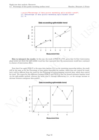
title(main="Data exceeding split-middle trend")
# Split-middle trend
lines(indep[1:n_a],sm.trend[1:n_a])
lines(indep[(n_a+1):nsize],projected[1:(nsize-n_a)])
# Print information
print("Percentage of data points exceeding split-middle trend");
print(pem_t)
Page 288](https://image.slidesharecdn.com/635a0af9-e378-45de-b512-1e1e88e419b8-160210073243/85/Tutorial-292-320.jpg)
![No
com
m
ercialuse
Single-case data analysis: Resources
16.6 Percentage of data points exceeding median trend Manolov, Moeyaert, & Evans
Code ends here. Default output of the code below:
1 2 3 4 5 6 7 8
2468101214
Measurement time
Score
Data exceeding split−middle trend
## [1] "Percentage of data points exceeding split-middle trend"
## [1] 75
Return to main text in the Tutorial about the Percentage of data points exceeding median trend: section
4.7.
Page 289](https://image.slidesharecdn.com/635a0af9-e378-45de-b512-1e1e88e419b8-160210073243/85/Tutorial-293-320.jpg)
![No
com
m
ercialuse
Single-case data analysis: Resources
16.7 Percentage of nonoverlapping corrected data Manolov, Moeyaert, & Evans
16.7 Percentage of nonoverlapping corrected data
After inputting the data actually obtained and specifying the aim of the intervention with respect to the target
behavior, the rest of the code is only copied and pasted.
# Input data: values in () separated by commas
phaseA <- c(9,8,8,7,6,7,7,6,6,5)
phaseB <- c(5,6,4,3,3,6,2,2,2,1)
# Specify whether the aim is to increase or reduce the behavior
aim<- 'increase' # Alternatively 'reduce'
# Copy and paste the rest of the code in the R console
n_a <- length(phaseA)
n_b <- length(phaseB)
# Data correction: phase A
phaseAdiff <- c(1:(n_a-1))
for (iter1 in 1:(n_a-1))
phaseAdiff[iter1] <- phaseA[iter1+1] - phaseA[iter1]
phaseAcorr <- c(1:n_a)
for (iter2 in 1:n_a)
phaseAcorr[iter2] <- phaseA[iter2] - mean(phaseAdiff)*iter2
# Data correction: phase B
phaseBcorr <- c(1:n_b)
for (iter3 in 1:n_b)
phaseBcorr[iter3] <- phaseB[iter3] - mean(phaseAdiff)*(iter3+n_a)
#################################################
# Represent graphically actual and detrended data
A_pred <- rep(0,n_a)
A_pred[1] <- phaseA[1]
for (i in 2:n_a)
A_pred[i] <- A_pred[i-1]+mean(phaseAdiff)
B_pred <- rep(0,n_b)
B_pred[1] <- A_pred[n_a] + mean(phaseAdiff)
for (i in 2:n_b)
B_pred[i] <- B_pred[i-1]+mean(phaseAdiff)
if (aim=="increase") reference <- max(phaseAcorr)
if (aim=="reduce") reference <- min(phaseAcorr)
slength <- n_a + n_b
info <- c(phaseA,phaseB)
time <- c(1:slength)
par(mfrow=c(2,1))
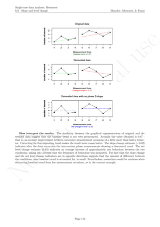
Page 290](https://image.slidesharecdn.com/635a0af9-e378-45de-b512-1e1e88e419b8-160210073243/85/Tutorial-294-320.jpg)
![No
com
m
ercialuse
Single-case data analysis: Resources
16.7 Percentage of nonoverlapping corrected data Manolov, Moeyaert, & Evans
plot(time,info, xlim=c(1,slength), ylim=c((min(info)-1),(max(info)+1)),
xlab="Measurement time", ylab="Variable of interest", font.lab=2)
abline(v=(n_a+0.5))
lines(time[1:n_a],info[1:n_a])
lines(time[1:n_a],A_pred[1:n_a],lty="dashed",col="green")
lines(time[(n_a+1):slength],info[(n_a+1):slength])
lines(time[(n_a+1):slength],B_pred,lty="dashed",col="red")
axis(side=1, at=seq(0,slength,1),labels=TRUE, font=2)
#axis(side=2, at=seq((min(info)-1),(max(info)+1),2),labels=TRUE, font=2)
points(time, info, pch=24, bg="black")
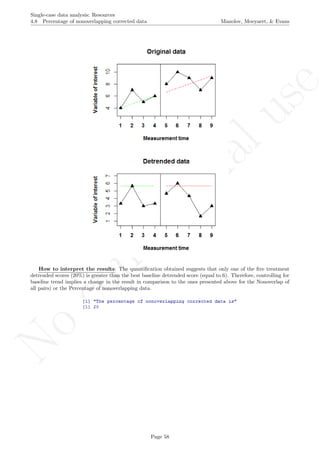
title (main="Original data")
transf <- c(phaseAcorr,phaseBcorr)
plot(time,transf, xlim=c(1,slength), ylim=c((min(transf)-1),(max(transf)+1)),
xlab="Measurement time", ylab="Variable of interest", font.lab=2)
abline(v=(n_a+0.5))
lines(time[1:n_a],transf[1:n_a])
lines(time[1:n_a],rep(reference,n_a),lty="dashed",col="green")
lines(time[(n_a+1):slength],rep(reference,n_b),lty="dashed",col="red")
lines(time[(n_a+1):slength],transf[(n_a+1):slength])
axis(side=1, at=seq(0,slength,1),labels=TRUE, font=2)
#axis(side=2, at=seq((min(transf)-1),(max(transf)+1),2),labels=TRUE, font=2)
points(time, transf, pch=24, bg="black")
title (main="Detrended data")
#####################################################
# PERFORM THE CALCULATIONS AND PRINT THE RESULT
# PND on corrected data: Aim to increase
if (aim == "increase")
{
countcorr <- 0
for (iter4 in 1:n_b)
if (phaseBcorr[iter4] > max(phaseAcorr))
+ countcorr <- countcorr+1
pndcorr <- (countcorr/n_b)*100
print ("The percent of nonoverlapping corrected data is");
print(pndcorr)
}
# PND on corrected data: Aim to reduce
if (aim == "reduce")
{
countcorr <- 0
for (iter4 in 1:n_b)
if (phaseBcorr[iter4] < min(phaseAcorr))
+ countcorr <- countcorr+1
pndcorr <- (countcorr/n_b)*100
print ("The percent of nonoverlapping corrected data is");
print(pndcorr)
}
Page 291](https://image.slidesharecdn.com/635a0af9-e378-45de-b512-1e1e88e419b8-160210073243/85/Tutorial-295-320.jpg)
![No
com
m
ercialuse
Single-case data analysis: Resources
16.7 Percentage of nonoverlapping corrected data Manolov, Moeyaert, & Evans
Code ends here. Default output of the code below:
5 10 15 20
0246810
Measurement time
Variableofinterest
1 2 3 4 5 6 7 8 9 11 13 15 17 19
Original data
5 10 15 20
791113
Measurement time
Variableofinterest
1 2 3 4 5 6 7 8 9 11 13 15 17 19
Detrended data
## [1] "The percent of nonoverlapping corrected data is"
## [1] 0
Return to main text in the Tutorial about the Percentage of nonoverlapping corrected data: section 4.8.
Page 292](https://image.slidesharecdn.com/635a0af9-e378-45de-b512-1e1e88e419b8-160210073243/85/Tutorial-296-320.jpg)
![No
com
m
ercialuse
Single-case data analysis: Resources
16.8 Percentage of zero data Manolov, Moeyaert, & Evans
16.8 Percentage of zero data
After inputting the data actually obtained, the rest of the code is only copied and pasted.
# Input data: values in () separated by commas
# n_a denotes number of baseline phase measurements
score <- c(7,5,6,7,5,4,0,1,0,2)
n_a <- 5
# Copy and paste the rest of the code in the R console
# Data manipulations
n_b <- length(score)-n_a
phaseA <- score[1:n_a]
phaseB <- score[(n_a+1):length(score)]
# PZD
counter_0 <- 0
counter_after <- 0
for (i in 1:n_b)
{
if (score[n_a+i]==0)
{
counter_0 <- counter_0 + 1
counter_after <- counter_after + 1
}
if ((score[n_a+i]!=0) && (counter_0 !=0))
counter_after <- counter_after + 1
}
# Plot data
indep <- 1:length(score)
plot(indep,score, xlim=c(indep[1],indep[length(indep)]),
xlab="Measurement time", ylab="Score", font.lab=2)
abline (v=(n_a+0.5))
for (i in 1:length(score)) if (score[i] == 0)
points(indep[i], score[i], pch=16, col="red")
for (i in 1:length(score)) if (score[i] != 0)
points(indep[i], score[i], pch=24, bg="black")
lines(indep[1:n_a],score[1:n_a],lty=2)
lines(indep[(n_a+1):length(score)],
score[(n_a+1):length(score)],lty=2)
pzd <- (counter_0 / counter_after)*100
print("Percentage of zero data after first
intervention 0 is achieved"); print(pzd)
Page 293](https://image.slidesharecdn.com/635a0af9-e378-45de-b512-1e1e88e419b8-160210073243/85/Tutorial-297-320.jpg)
![No
com
m
ercialuse
Single-case data analysis: Resources
16.8 Percentage of zero data Manolov, Moeyaert, & Evans
Code ends here. Default output of the code below:
2 4 6 8 10
01234567
Measurement time
Score
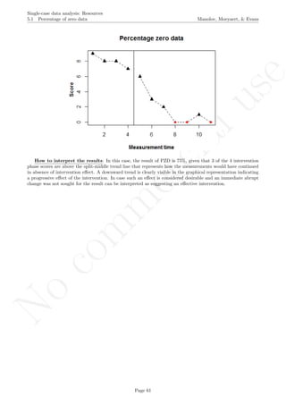
## [1] "Percentage of zero data after first intervention 0 is achieved"
## [1] 50
Return to main text in the Tutorial about the Percentage Zero Data: 5.1.
Page 294](https://image.slidesharecdn.com/635a0af9-e378-45de-b512-1e1e88e419b8-160210073243/85/Tutorial-298-320.jpg)
![No
com
m
ercialuse
Single-case data analysis: Resources
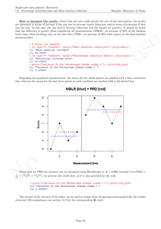
16.9 Percentage change index Manolov, Moeyaert, & Evans
16.9 Percentage change index
Percentage change index is the general name for the two indices included in the code. They have also been
called Percentage reduction data (when focusing on the last three measurements for each phase) and Mean
baseline reduction (when using all data).
After inputting the data actually obtained, the rest of the code is only copied and pasted.
# Input data: values in () separated by commas
# n_a denotes number of baseline phase measurements
score <- c(5,6,7,5,5,7,7,6,8,9,7)
n_a <- 5
# Specify whether the aim is to increase or reduce the behavior
aim<- 'increase' # Alternatively 'reduce'
# Copy and paste the rest of the code in the R console
# Data manipulations
n_b <- length(score)-n_a
phaseA <- score[1:n_a]
phaseB <- score[(n_a+1):length(score)]
# Mean baseline reduction
mblr <- ((mean(phaseB)-mean(phaseA))/mean(phaseA))*100
# Percentage reduction data
sum_a <- 0
for (i in (n_a-2):n_a)
sum_a <- sum_a + phaseA[i]
sum_b <- 0
for (i in (n_b-2):n_b)
sum_b <- sum_b + phaseB[i]
prd <- ((sum_b/3 - sum_a/3)/(sum_a/3))*100
# Compute the variance of PRD
mean_a <- sum_a/3
mean_b <- sum_b/3
var_prd <- ( ((var(phaseA)+var(phaseB))/3) +
+ ((mean_a-mean_b)^2/2) )/ var(phaseA)
# Graphical representation
# Plot data
indep <- 1:length(score)
plot(indep,score, xlim=c(indep[1],indep[length(indep)]),
xlab="Measurement time", ylab="Score", font.lab=2)
lines(indep[1:n_a],score[1:n_a],lty=2)
lines(indep[(n_a+1):length(score)],
score[(n_a+1):length(score)],lty=2)
abline (v=(n_a+0.5))
points(indep, score, pch=24, bg="black")
Page 295](https://image.slidesharecdn.com/635a0af9-e378-45de-b512-1e1e88e419b8-160210073243/85/Tutorial-299-320.jpg)
![No
com
m
ercialuse
Single-case data analysis: Resources
16.9 Percentage change index Manolov, Moeyaert, & Evans
title(main="MBLR [blue] + PRD [red]")
# Add lines
lines(indep[1:n_a],rep(mean(phaseA),n_a),col="blue")
lines(indep[(n_a+1):length(score)],
rep(mean(phaseB),n_b),col="blue")
lines(indep[(n_a-2):n_a],rep((sum_a/3),3),
col="red",lwd=3,lty="dashed")
lines(indep[(n_a+n_b-2):length(score)],
rep((sum_b/3),3),col="red",lwd=3)
# Print the results
if (aim == "reduce") {print("Mean baseline reduction");
print(mblr)} else {print("Mean baseline increase");
print(mblr)}
if (aim == "reduce") {print("Percentage reduction data");
print(prd)} else {print("Percentage increase data");
print(prd)}
print("Variance of the Percentage change index = ");
print(var_prd)
Page 296](https://image.slidesharecdn.com/635a0af9-e378-45de-b512-1e1e88e419b8-160210073243/85/Tutorial-300-320.jpg)
![No
com
m
ercialuse
Single-case data analysis: Resources
16.9 Percentage change index Manolov, Moeyaert, & Evans
Code ends here. Default output of the code below:
2 4 6 8 10
56789
Measurement time
Score
MBLR [blue] + PRD [red]
## [1] "Mean baseline increase"
## [1] 30.95238
## [1] "Percentage increase data"
## [1] 41.17647
## [1] "Variance of the Percentage change index = "
## [1] 4.180556
Return to main text in the Tutorial about the Percentage change index (Percentage reduction data and
Mean baseline reduction): section 5.2.
Page 297](https://image.slidesharecdn.com/635a0af9-e378-45de-b512-1e1e88e419b8-160210073243/85/Tutorial-301-320.jpg)
![No
com
m
ercialuse
Single-case data analysis: Resources
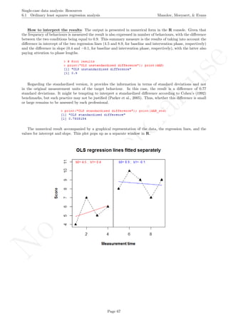
16.10 Ordinary least squares regression analysis Manolov, Moeyaert, & Evans
16.10 Ordinary least squares regression analysis
Only the descriptive information (i.e., coefficient estimates) of the OLS regression is used here, not the inferential
information (i.e., statistical significance of these estimates).
After inputting the data actually obtained, the rest of the code is only copied and pasted.
# Input data: values in () separated by commas
# n_a denotes number of baseline phase measurements
score <- c(4,3,3,8,3,5,6,7,7,6)
n_a <- 5
# Copy and paste the rest of the code in the R console
# Create necessary objects
nsize <- length(score)
n_b <- nsize - n_a
phaseA <- score[1:n_a]
phaseB <- score[(n_a+1):nsize]
time_A <- 1:n_a
time_B <- 1:n_b
# Phase A: regressor = time
reg_A <- lm(phaseA ~ time_A)
# Phase B: regressor = time
reg_B <- lm(phaseB ~ time_B)
# Plot data
indep <- 1:length(score)
plot(indep,score, xlim=c(indep[1],indep[length(indep)]),
ylim=c(min(score),max(score)+1/10*max(score)),
xlab="Measurement time", ylab="Score", font.lab=2)
lines(indep[1:n_a],score[1:n_a],lty=2)
lines(indep[(n_a+1):length(score)],
score[(n_a+1):length(score)],lty=2)
abline (v=(n_a+0.5))
points(indep, score, pch=24, bg="black")
title(main="OLS regression lines fitted separately")
lines(indep[1:n_a],reg_A$fitted,col="red")
lines(indep[(n_a+1):length(score)],reg_B$fitted,col="blue")
text(0.8,(max(score)+1/10*max(score)),
paste("b0=",round(reg_A$coefficients[[1]],digits=2),"; ",
"b1=",round(reg_A$coefficients[[2]],digits=2)),
pos=4,cex=0.8,col="red")
text(n_a+0.8,(max(score)+1/10*max(score)),
paste("b0=",round(reg_B$coefficients[[1]],digits=2),"; ",
"b1=",round(reg_B$coefficients[[2]],digits=2)),
pos=4,cex=0.8,col="blue")
# Compute values
dAB <- reg_B$coefficients[[1]] - reg_A$coefficients[[1]] +
(reg_B$coefficients[[2]]-reg_A$coefficients[[2]])*
((n_a+1+n_a + n_b)/2)
res <- sqrt( ((n_a-1)*var(reg_A$residuals) +
(n_b-1)*var(reg_B$residuals)) / (n_a+n_b-2))
dAB_std <- dAB/res
Page 298](https://image.slidesharecdn.com/635a0af9-e378-45de-b512-1e1e88e419b8-160210073243/85/Tutorial-302-320.jpg)

![No
com
m
ercialuse
Single-case data analysis: Resources
16.10 Ordinary least squares regression analysis Manolov, Moeyaert, & Evans
Code ends here. Default output of the code below:
2 4 6 8 10
3456789
Measurement time
Score
OLS regression lines fitted separately
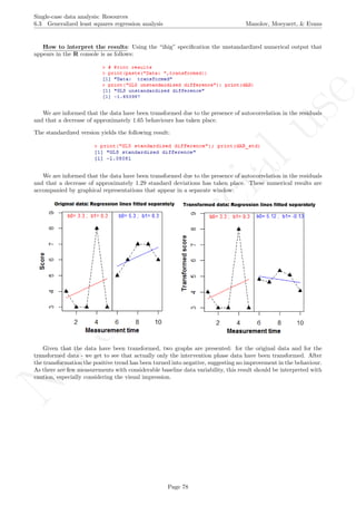
b0= 3.3 ; b1= 0.3 b0= 5.3 ; b1= 0.3
## [1] "OLS unstandardized difference"
## [1] 2
## [1] "OLS standardized difference"
## [1] 1.271283
Return to main text in the Tutorial about the Ordinary least squares effect size: section 6.1.
Page 300](https://image.slidesharecdn.com/635a0af9-e378-45de-b512-1e1e88e419b8-160210073243/85/Tutorial-304-320.jpg)
![No
com
m
ercialuse
Single-case data analysis: Resources
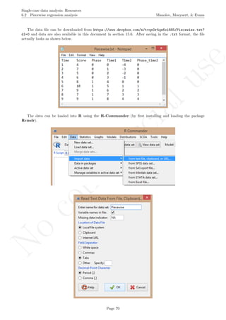
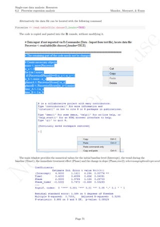
16.11 Piecewise regression analysis Manolov, Moeyaert, & Evans
16.11 Piecewise regression analysis
Only the descriptive information (i.e., coefficient estimates) of the Piecewise regression is used here, not the
inferential information (i.e., statistical significance of these estimates).
After inputting the data actually obtained, the rest of the code is only copied and pasted.
Code for analysis created by Mariola Moeyaert; code for the graphical representation created by Rumen
Manolov.
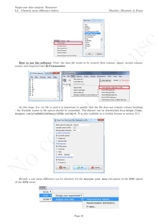
# Input data: copy-paste line and load/locate the data matrix
Piecewise <- read.table(file.choose(), header=TRUE)
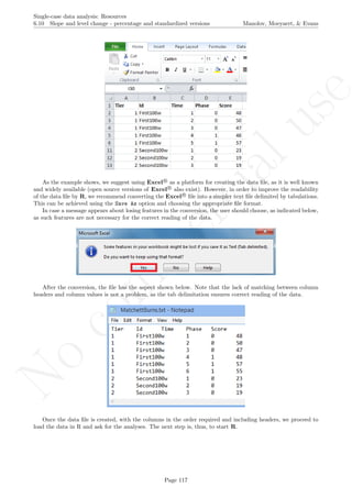
Data matrix aspect as shown below:
## Time Score Phase Time1 Time2 Phase_time2
## 1 4 0 0 -4 0
## 2 7 0 1 -3 0
## 3 5 0 2 -2 0
## 4 6 0 3 -1 0
## 5 8 1 4 0 0
## 6 10 1 5 1 1
## 7 9 1 6 2 2
## 8 7 1 7 3 3
## 9 9 1 8 4 4
# Copy and paste the rest of the code in the R console
# Create necessary objects
nsize <- nrow(Piecewise)
n_a <- 0
for (i in 1:nsize)
if (Piecewise$Phase[i]==0) n_a <- n_a + 1
n_b <- nsize - n_a
phaseA <- Piecewise$Score[1:n_a]
phaseB <- Piecewise$Score[(n_a+1):nsize]
time_A <- 1:n_a
time_B <- 1:n_b
# Unstandardized
# Piecewise regression
reg <- lm(Score ~ Time1 + Phase + Phase_time2, Piecewise)
summary(reg)
res <- sqrt(deviance(reg)/df.residual(reg))
# Compute unstandardized effect sizes
Chance_Level <- reg$coefficients[[3]]
Chance_Slope <- reg$coefficients[[4]]
# Compute standardized effect sizes
Chance_Level_s = reg$coefficients[[3]]/res;
Chance_Slope_s = reg$coefficients[[4]]/res;
# Standardize the results
baseline.scores_std <- rep(0,n_a)
Page 301](https://image.slidesharecdn.com/635a0af9-e378-45de-b512-1e1e88e419b8-160210073243/85/Tutorial-305-320.jpg)
![No
com
m
ercialuse
Single-case data analysis: Resources
16.11 Piecewise regression analysis Manolov, Moeyaert, & Evans
intervention.scores_std <- rep(0,n_b)
for (i in 1:n_a)
baseline.scores_std[i] <- Piecewise$Score[i]/res
for (i in 1:n_b)
intervention.scores_std[i] <- Piecewise$Score[n_a+i]/res
scores_std <- rep(0,nsize)
for (i in 1:nsize)
scores_std[i] <- Piecewise$Score[i]/res
Piecewise_std <- cbind(Piecewise,scores_std)
# Plot data
indep <- 1:nsize
proj <- reg$coefficients[[1]]+reg$coefficients[[2]]*
+ Piecewise$Time1[n_a+1]
plot(indep,Piecewise$Score, xlim=c(indep[1],indep[nsize]),
xlab="Time1", ylab="Score", font.lab=2,xaxt="n")
axis(side=1, at=seq(1,nsize,1),labels=Piecewise$Time1, font=2)
lines(indep[1:n_a],Piecewise$Score[1:n_a],lty=2)
lines(indep[(n_a+1):length(Piecewise$Score)],
Piecewise$Score[(n_a+1):length(Piecewise$Score)],lty=2)
abline (v=(n_a+0.5))
points(indep, Piecewise$Score, pch=24, bg="black")
title(main="Piecewise regression: Unstandardized effects")
lines(indep[1:(n_a+1)],c(reg$fitted[1:n_a],proj),col="red")
lines(indep[(n_a+1):length(Piecewise$Score)],
reg$fitted[(n_a+1):length(Piecewise$Score)],col="red")
text(1,reg$coefficients[[1]],paste(round(reg$coefficients[[1]],
digits=2)),col="blue")
if (n_a%%2 == 0) middle <- n_a/2
if (n_a%%2 == 1) middle <- (n_a+1)/2
lines(indep[middle:(middle+1)],rep(reg$fitted[middle],2),
col="darkgreen")
lines(rep(indep[middle+1],2),reg$fitted[middle:(middle+1)],
col="darkgreen",lwd=4)
text((middle+1.5),(reg$fitted[middle]+0.5*(reg$coefficients[[2]])),
paste(round(reg$coefficients[[2]],digits=2)),col="darkgreen")
if (n_b%%2 == 0) middleB <- n_a + n_b/2
if (n_b%%2 == 1) middleB <- n_a + (n_b+1)/2
lines(indep[middleB:(middleB+1)],rep(reg$fitted[middleB],2),
col="darkgreen")
lines(rep(indep[middleB+1],2),reg$fitted[middleB:(middleB+1)],
col="darkgreen",lwd=4)
lines(indep[middleB:(middleB+1)],
c(reg$fitted[middleB],(reg$fitted[middleB]+(reg$coefficients[[2]]))),
col="green")
lines(rep(indep[middleB+1],2),
c((reg$fitted[middleB]+ (reg$coefficients[[2]])),reg$fitted[middleB]),
col="green",lwd=4)
text((middleB+1.5),
(reg$fitted[middleB]+(reg$coefficients[[2]])),
paste(round(reg$coefficients[[4]],digits=2)),col="red")
text((middleB+1.5),
(reg$fitted[middleB]+0.5*(reg$coefficients[[4]])),
paste(round((reg$coefficients[[4]]+reg$coefficients[[2]]),
digits=2)),col="darkgreen")
lines(rep(indep[n_a+1],2),c(proj,reg$fitted[n_a+1]),col="blue",lwd=4)
Page 302](https://image.slidesharecdn.com/635a0af9-e378-45de-b512-1e1e88e419b8-160210073243/85/Tutorial-306-320.jpg)
![No
com
m
ercialuse
Single-case data analysis: Resources
16.11 Piecewise regression analysis Manolov, Moeyaert, & Evans
text((n_a+1.5),(proj+0.5*(reg$fitted[n_a+1]-proj)),
paste(round(reg$coefficients[[3]],digits=2)),col="blue")
# Print standardized data
print("Standardized baseline data");
print(baseline.scores_std)
print("Standardized intervention phase data");
print(intervention.scores_std)
write.table(Piecewise_std, "Standardized_data.txt",
sep="t",row.names=FALSE)
# Print results
print("Piecewise unstandardized immediate treatment effect");
print(Chance_Level)
print("Piecewise unstandardized change in slope");
print(Chance_Slope)
# Print results
print("Piecewise standardized immediate treatment effect");
print(Chance_Level_s)
print("Piecewise standardized change in slope");
print(Chance_Slope_s)
Page 303](https://image.slidesharecdn.com/635a0af9-e378-45de-b512-1e1e88e419b8-160210073243/85/Tutorial-307-320.jpg)
![No
com
m
ercialuse
Single-case data analysis: Resources
16.11 Piecewise regression analysis Manolov, Moeyaert, & Evans
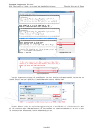
Code ends here. Default output of the code below:
##
## Call:
## lm(formula = Score ~ Time1 + Phase + Phase_time2, data = Piecewise)
##
## Residuals:
## 1 2 3 4 5 6 7 8 9
## -0.9 1.7 -0.7 -0.1 -0.8 1.3 0.4 -1.5 0.6
##
## Coefficients:
## Estimate Std. Error t value Pr(>|t|)
## (Intercept) 4.9000 1.1411 4.294 0.00776 **
## Time1 0.4000 0.6099 0.656 0.54091
## Phase 2.3000 1.9764 1.164 0.29703
## Phase_time2 -0.5000 0.7470 -0.669 0.53293
## ---
## Signif. codes: 0 '***' 0.001 '**' 0.01 '*' 0.05 '.' 0.1 ' ' 1
##
## Residual standard error: 1.364 on 5 degrees of freedom
## Multiple R-squared: 0.7053,Adjusted R-squared: 0.5285
## F-statistic: 3.988 on 3 and 5 DF, p-value: 0.08529
## [1] " "
Page 304](https://image.slidesharecdn.com/635a0af9-e378-45de-b512-1e1e88e419b8-160210073243/85/Tutorial-308-320.jpg)
![No
com
m
ercialuse
Single-case data analysis: Resources
16.11 Piecewise regression analysis Manolov, Moeyaert, & Evans
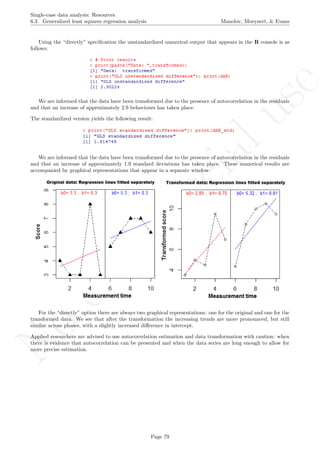
45678910
Time1
Score
0 1 2 3 4 5 6 7 8
Piecewise regression: Unstandardized effects
4.9
0.4
−0.5
−0.1
2.3
## [1] "Standardized baseline data"
## [1] 2.932942 5.132649 3.666178 4.399413
## [1] "Standardized intervention phase data"
## [1] 5.865885 7.332356 6.599120 5.132649 6.599120
## [1] " "
## [1] "Piecewise unstandardized immediate treatment effect"
## [1] 2.3
## [1] "Piecewise unstandardized change in slope"
## [1] -0.5
## [1] " "
## [1] "Piecewise standardized immediate treatment effect"
## [1] 1.686442
## [1] "Piecewise standardized change in slope"
## [1] -0.3666178
Document with standardized data also created:
Return to main text in the Tutorial about the Piecewise regression effect size: section 6.2.
Page 305](https://image.slidesharecdn.com/635a0af9-e378-45de-b512-1e1e88e419b8-160210073243/85/Tutorial-309-320.jpg)
![No
com
m
ercialuse
Single-case data analysis: Resources
16.12 Generalized least squares regression analysis Manolov, Moeyaert, & Evans
16.12 Generalized least squares regression analysis
Only the descriptive information (i.e., coefficient estimates) of the GLS regression is used here, not the inferential
information (i.e., statistical significance of these estimates). Statistical significance is only tested for the residuals
via the Durbin-Watson test.
After inputting the data actually obtained, the rest of the code is only copied and pasted.
This code requires that the lmtest package for R (which it loads). In case it has not been previously installed,
this is achieved in the R console via the following code:
install.packages('lmtest')
Once the package is installed, the rest of the code is used, as follows:
# Input data: values in () separated by commas
# n_a denotes number of baseline phase measurements
score <- c(4,7,5,6,8,10,9,7,9)
n_a <- 4
# Choose how to deal with autocorrelation
# "directly" - uses the Cochran-Orcutt estimation
# and transforms data prior to using them as in
# Generalized least squares by Swaminathan et al. (2010)
# "ifsig" - uses Durbin-Watson test and only if the
# transforms data, as in Autoregressive analysis by Gorsuch (1983)
transform<- 'ifsig' # Alternatively 'directly'
# Copy and paste the rest of the code in the R console
require(lmtest)
# Create necessary objects
nsize <- length(score)
n_b <- nsize - n_a
phaseA <- score[1:n_a]
phaseB <- score[(n_a+1):nsize]
time_A <- 1:n_a
time_B <- 1:n_b
#####################
if (transform == "directly")
{
transformed <- "transformed"
tiempo <- 1:length(score)
# Whole series regression for checking
# autocorr between residuals
whole1 <- summary( lm (score ~ tiempo))
whole2 <- whole1[[4]]
pred.whole <- rep(0,nsize)
res.whole <- rep(0,nsize)
for (i in 1:nsize)
Page 306](https://image.slidesharecdn.com/635a0af9-e378-45de-b512-1e1e88e419b8-160210073243/85/Tutorial-310-320.jpg)
![No
com
m
ercialuse
Single-case data analysis: Resources
16.12 Generalized least squares regression analysis Manolov, Moeyaert, & Evans
pred.whole[i] <- whole2[1,1] + whole2[2,1]*tiempo[i]
for (i in 1:nsize)
res.whole[i] <- score[i] - pred.whole[i]
# Estimate autocorrelation
# through regression among residuals
dv <- res.whole[2:nsize]
iv <- res.whole[1:(nsize-1)]
residu1 <- summary(lm(dv ~ 0 + iv)) # No intercept
residu2 <- residu1[[4]]
ac_estimate <- residu2[1,1]
# Create the vectors for each phase: to be used in GLS
phaseA_transf <- rep(0,n_a)
timeA_transf <- rep(0,n_a)
phaseB_transf <- rep(0,n_b)
timeB_transf <- rep(0,n_b)
# Transform data (Y=measurements) (tiempo=TREND predictor)
ytransf <- rep(0,nsize)
trendtrans <- rep(0,nsize)
# Prais-Winston for the first data point
# (in order not to lose any!)
phaseA_transf[1] <- score[1]*sqrt(1-ac_estimate*ac_estimate)
phaseB_transf[1] <- score[n_a+1]*sqrt(1-ac_estimate*ac_estimate)
timeA_transf[1] <- tiempo[1]*sqrt(1-ac_estimate*ac_estimate)
timeB_transf[1] <- tiempo[1]*sqrt(1-ac_estimate*ac_estimate)
# Transform remaining
# Assign values to the phases
for (i in 2:n_a)
{
phaseA_transf[i] <- score[i] - ac_estimate*score[i-1]
timeA_transf[i] <- tiempo[i] - ac_estimate*tiempo[i-1]
}
for (i in 2:n_b)
{
phaseB_transf[i] <- score[n_a+i] - ac_estimate*score[n_a+i-1]
timeB_transf[i] <- tiempo[i] - ac_estimate*tiempo[i-1]
}
# Phase A: regressor = time
reg_A_transf <- lm(phaseA_transf ~ timeA_transf)
# Phase B: regressor = time
reg_B_transf <- lm(phaseB_transf ~ timeB_transf)
dAB <- reg_B_transf$coefficients[[1]] -
+ reg_A_transf$coefficients[[1]] +
+ (reg_B_transf$coefficients[[2]]-
+ reg_A_transf$coefficients[[2]])*((n_a+1+n_a + n_b)/2)
res <- sqrt( ((n_a-1)*var(reg_A_transf$residuals) +
+ (n_b-1)*var(reg_B_transf$residuals)) / (n_a+n_b-2))
dAB_std <- dAB/res
}
#####################
Page 307](https://image.slidesharecdn.com/635a0af9-e378-45de-b512-1e1e88e419b8-160210073243/85/Tutorial-311-320.jpg)
![No
com
m
ercialuse
Single-case data analysis: Resources
16.12 Generalized least squares regression analysis Manolov, Moeyaert, & Evans
if (transform == "ifsig")
{
# Phase A: regressor = time
reg_A <- lm(phaseA ~ time_A)
# Phase B: regressor = time
reg_B <- lm(phaseB ~ time_B)
# Durbin-Watson test of autocorrelation
DWstat_A <- dwtest(phaseA ~ time_A)
DWstat_B <- dwtest(phaseB ~ time_B)
# Estimate autocorrelation through the DW statistic
autocor_A <- 1-(DWstat_A$statistic/2)
autocor_A
autocor_B <- 1-(DWstat_B$statistic/2)
autocor_B
# Transform or not acc to whether autcorrelation is sig
if (DWstat_A$p.value <= 0.05)
{
transformed <- "transformed"
phaseA_transf <- 1:n_a
phaseB_transf <- 1:n_b
timeA_transf <- 1:n_a
timeB_transf <- 1:n_b
phaseA_transf[1] <- score[1]*sqrt(1-autocor_A[[1]]*
+ autocor_A[[1]])
timeA_transf[1] <- time_A[1]*sqrt(1-autocor_A[[1]]*
+ autocor_A[[1]])
for (i in 2:n_a)
{
phaseA_transf[i] <- score[i] - autocor_A[[1]]*score[i-1]
timeA_transf[i] <- time_A[i] - autocor_A[[1]]*time_A[i-1]
}
phaseB_transf <- phaseB
timeB_transf <- time_B
}
if (DWstat_B$p.value <= 0.05)
{
transformed <- "transformed"
phaseA_transf <- 1:n_a
phaseB_transf <- 1:n_b
timeA_transf <- 1:n_a
timeB_transf <- 1:n_b
phaseA_transf <- phaseA
timeA_transf <- time_A
timeB_transf[1] <- time_B[1]*sqrt(1-autocor_B[[1]]*
+ autocor_B[[1]])
phaseB_transf[1] <- score[n_a+1]*sqrt(1-autocor_B[[1]]*
+ autocor_B[[1]])
for (i in 2:n_b)
{
Page 308](https://image.slidesharecdn.com/635a0af9-e378-45de-b512-1e1e88e419b8-160210073243/85/Tutorial-312-320.jpg)
![No
com
m
ercialuse
Single-case data analysis: Resources
16.12 Generalized least squares regression analysis Manolov, Moeyaert, & Evans
phaseB_transf[i] <- score[n_a+i] - autocor_B[[1]]*
+ score[n_a+i-1]
timeB_transf[i] <- time_B[i] - autocor_B[[1]]*time_B[i-1]
}
}
if ((DWstat_A$p.value <= 0.05) || (DWstat_B$p.value <= 0.05))
{
ytransf <- c(phaseA_transf,phaseB_transf)
# Phase A: regressor = time
reg_A_transf <- lm(phaseA_transf ~ timeA_transf)
# Phase B: regressor = time
reg_B_transf <- lm(phaseB_transf ~ timeB_transf)
dAB <- reg_B_transf$coefficients[[1]] -
+ reg_A_transf$coefficients[[1]] +
+ (reg_B_transf$coefficients[[2]] -
+ reg_A_transf$coefficients[[2]])*
+ ((n_a+1+n_a + n_b)/2)
res <- sqrt( ((n_a-1)*var(reg_A_transf$residuals) +
+ (n_b-1)*var(reg_B_transf$residuals)) / (n_a+n_b-2))
dAB_std <- dAB/res
}
if ((DWstat_A$p.value > 0.05) && (DWstat_B$p.value > 0.05))
{
transformed <- "original"
# Regression with original data
dAB <- reg_B$coefficients[[1]] - reg_A$coefficients[[1]] +
+ (reg_B$coefficients[[2]]-reg_A$coefficients[[2]])*
+ ((n_a+1+n_a + n_b)/2)
res <- sqrt( ((n_a-1)*var(reg_A$residuals) + (n_b-1)*
+ var(reg_B$residuals)) / (n_a+n_b-2))
dAB_std <- dAB/res
}
}
#################################
# Graphical representation
if (transformed == "original")
{
# Plot data
indep <- 1:length(score)
plot(indep,score, xlim=c(indep[1],indep[length(indep)]),
ylim=c(min(score),max(score)+1/10*max(score)),
xlab="Measurement time", ylab="Score", font.lab=2)
lines(indep[1:n_a],score[1:n_a],lty=2)
lines(indep[(n_a+1):length(score)],
score[(n_a+1):length(score)],lty=2)
abline (v=(n_a+0.5))
points(indep, score, pch=24, bg="black")
title(main="Original data:Regression lines fitted separately")
# Add lines
Page 309](https://image.slidesharecdn.com/635a0af9-e378-45de-b512-1e1e88e419b8-160210073243/85/Tutorial-313-320.jpg)
![No
com
m
ercialuse
Single-case data analysis: Resources
16.12 Generalized least squares regression analysis Manolov, Moeyaert, & Evans
lines(indep[1:n_a],reg_A$fitted,col="red")
lines(indep[(n_a+1):length(score)],reg_B$fitted,col="blue")
text(0.8,(max(score)+1/10*max(score)),
paste("b0=",round(reg_A$coefficients[[1]],digits=2),"; ",
"b1=",round(reg_A$coefficients[[2]],digits=2)),
pos=4,cex=0.8,col="red")
text(n_a+0.8,(max(score)+1/10*max(score)),
paste("b0=",round(reg_B$coefficients[[1]],digits=2),"; ",
"b1=",round(reg_B$coefficients[[2]],digits=2)),
pos=4,cex=0.8,col="blue")
}
if (transformed == "transformed")
{
par(mfrow=c(1,2))
indep <- 1:length(score)
plot(indep,score, xlim=c(indep[1],indep[length(indep)]),
ylim=c(min(score),max(score)+1/10*max(score)),
xlab="Measurement time", ylab="Score", font.lab=2)
lines(indep[1:n_a],score[1:n_a],lty=2)
lines(indep[(n_a+1):length(score)],
score[(n_a+1):length(score)],lty=2)
abline (v=(n_a+0.5))
points(indep, score, pch=24, bg="black")
title(main="Original data: Regression lines fitted separately")
lines(indep[1:n_a],reg_A$fitted,col="red")
lines(indep[(n_a+1):length(score)],reg_B$fitted,col="blue")
text(0.8,(max(score)+1/10*max(score)),
paste("b0=",round(reg_A$coefficients[[1]],digits=2),"; ",
"b1=",round(reg_A$coefficients[[2]],digits=2)),
pos=4,cex=0.8,col="red")
text(n_a+0.8,(max(score)+1/10*max(score)),
paste("b0=",round(reg_B$coefficients[[1]],digits=2),"; ",
"b1=",round(reg_B$coefficients[[2]],digits=2)),
pos=4,cex=0.8,col="blue")
transfall <- c(phaseA_transf,phaseB_transf)
plot(indep,transfall, xlim=c(indep[1],indep[length(indep)]),
ylim=c(min(transfall),max(transfall)+1/10*max(transfall)),
xlab="Measurement time",ylab="Transformed score", font.lab=2)
lines(indep[1:n_a],phaseA_transf[1:n_a],lty=2)
lines(indep[(n_a+1):length(score)],phaseB_transf[1:n_b],lty=2)
abline (v=(n_a+0.5))
points(indep, ytransf, pch=24, bg="black")
title(main="Transformed data: Regression lines fitted separately")
lines(indep[1:n_a],reg_A_transf$fitted,col="red")
lines(indep[(n_a+1):length(score)],reg_B_transf$fitted,col="blue")
text(0.8,(max(transfall)+1/10*max(transfall)),
paste("b0=",round(reg_A_transf$coefficients[[1]],digits=2),"; ",
"b1=",round(reg_A_transf$coefficients[[2]],digits=2)),
pos=4,cex=0.8,col="red")
text(n_a+0.8,(max(transfall)+1/10*max(transfall)),
paste("b0=",round(reg_B_transf$coefficients[[1]],digits=2),"; ",
"b1=",round(reg_B_transf$coefficients[[2]],digits=2)),
pos=4,cex=0.8,col="blue")
}
# Print results
print(paste("Data: ",transformed))
Page 310](https://image.slidesharecdn.com/635a0af9-e378-45de-b512-1e1e88e419b8-160210073243/85/Tutorial-314-320.jpg)

![No
com
m
ercialuse
Single-case data analysis: Resources
16.12 Generalized least squares regression analysis Manolov, Moeyaert, & Evans
Code ends here. Default output of the code below:
## Loading required package: lmtest
## Loading required package: zoo
##
## Attaching package: ’zoo’
##
## The following objects are masked from ’package:base’:
##
## as.Date, as.Date.numeric
2 4 6 8
4567891011
Measurement time
Score
Original data:Regression lines fitted separately
b0= 4.5 ; b1= 0.4 b0= 8.9 ; b1= −0.1
## [1] "Data: original"
## [1] "GLS unstandardized difference"
## [1] 0.9
## [1] "GLS standardized difference"
## [1] 0.7808184
Return to main text in the Tutorial about the Generalized least squares regression analysis effect size: section
6.3.
Page 312](https://image.slidesharecdn.com/635a0af9-e378-45de-b512-1e1e88e419b8-160210073243/85/Tutorial-316-320.jpg)
![No
com
m
ercialuse
Single-case data analysis: Resources
16.13 Mean phase difference - original version (2013) Manolov, Moeyaert, & Evans
16.13 Mean phase difference - original version (2013)
This code refers to the first version of the MPD, as described in the Journal of School Psychology in 2013. This
version projects the estimated baseline trend into the treatment phase, starting from the last baseline phase
measurement. In contrast, the revised version of the MPD, as described in Neuropsychological Rehabilitation in
2015, which projects the estimated baseline trend into the treatment phase, according to the height / intercept
of the baseline phase trend (i.e., starting from the last fitted (not actual) baseline phase measurement occasion.
# Input data: values in () separated by commas
baseline <- c(1,2,3)
treatment <- c(5,6,7)
# Copy and paste the rest of the code in the R console
# Obtain phase length
n_a <- length(baseline)
n_b <- length(treatment)
# Estimate baseline trend
base_diff <- rep(0,(n_a-1))
for (i in 1:(n_a-1))
base_diff[i] <- baseline[i+1] - baseline[i]
trendA <- mean(base_diff)
# Project baseline trend to the treatment phase
treatment_pred <- rep(0,n_b)
for (i in 1:n_b)
treatment_pred[i] <- baseline[1] + trendA*(n_a+i-1)
# PERFORM THE CALCULATIONS
# Compare the predicted and the actually obtained
# treatment data and obtain the average difference
mpd <- mean(treatment-treatment_pred)
#######################
# Represent graphically the actual data
# and the projected treatment data
info <- c(baseline,treatment)
info_pred <- c(baseline,treatment_pred)
minimo <- min(info,info_pred)
maximo <- max(info,info_pred)
time <- c(1:length(info))
plot(time,info, xlim=c(1,length(info)),
ylim=c((minimo-1),(maximo+1)), xlab="Measurement time",
ylab="Behavior of interest", font.lab=2)
abline(v=(n_a+0.5))
lines(time[1:n_a],info[1:n_a])
lines(time[(n_a+1):length(info)],info[(n_a+1):length(info)])
axis(side=1, at=seq(0,length(info),1),labels=TRUE, font=2)
points(time, info, pch=24, bg="black")
points (time, info_pred, pch=19)
points (time, info_pred, pch=1)
lines(time[(n_a+1):length(info)],info_pred[(n_a+1):length(info)],lty="dashed")
title (main="Predicted (circle) vs. actual (triangle) data")
Page 313](https://image.slidesharecdn.com/635a0af9-e378-45de-b512-1e1e88e419b8-160210073243/85/Tutorial-317-320.jpg)

![No
com
m
ercialuse
Single-case data analysis: Resources
16.13 Mean phase difference - original version (2013) Manolov, Moeyaert, & Evans
Code ends here. Default output of the code below:
1 2 3 4 5 6
02468
Measurement time
Behaviorofinterest
1 2 3 4 5 6
Predicted (circle) vs. actual (triangle) data
Baseline trend = 1 . MPD = 1
## [1] "The mean phase difference is"
## [1] 1
Return to main text in the Tutorial about the original version of the Mean phase difference: section 6.7.
Page 315](https://image.slidesharecdn.com/635a0af9-e378-45de-b512-1e1e88e419b8-160210073243/85/Tutorial-319-320.jpg)

![No
com
m
ercialuse
Single-case data analysis: Resources
16.14 Mean phase difference - percentage version (2015) Manolov, Moeyaert, & Evans
## 3 Third100w 10 1 54
## 3 Third100w 11 1 47
## 3 Third100w 12 1 57
# Copy and paste the following code in the R console
# Whole number function
is.wholenumber<- function(x, tol=.Machine$double.eps^0.5) abs(x-round(x)) < tol
# Function for computing MPD, its percentage-version, and mean square error
mpd <- function(baseline,treatment)
{
# Obtain phase length
n_a <- length(baseline)
n_b <- length(treatment)
meanA <- mean(baseline)
# Estimate baseline trend
base_diff <- rep(0,(n_a-1))
for (i in 1:(n_a-1))
base_diff[i] <- baseline[i+1] - baseline[i]
trendA <- mean(base_diff)
# Predict baseline data
baseline_pred <- rep(0,n_a)
midX <- median(c(1:n_a))
midY <- median(baseline)
is.wholenumber <- function(x, tol = .Machine$double.eps^0.5) abs(x - round(x)) < tol
if (is.wholenumber(midX))
{
baseline_pred[midX] <- midY
for (i in (midX-1):1) baseline_pred[i] <- baseline_pred[i+1] - trendA
for (i in (midX+1):n_a) baseline_pred[i] <- baseline_pred[i-1] + trendA
}
if (!is.wholenumber(midX))
{
baseline_pred[midX-0.5] <- midY-(0.5*trendA)
baseline_pred[midX+0.5] <- midY+(0.5*trendA)
for (i in (midX-1.5):1) baseline_pred[i] <- baseline_pred[i+1] - trendA
for (i in (midX+1.5):n_a) baseline_pred[i] <- baseline_pred[i-1] + trendA
}
# Project baseline trend to the treatment phase
treatment_pred <- rep(0,n_b)
treatment_pred[1] <- baseline_pred[n_a] + trendA
for (i in 2:n_b)
treatment_pred[i] <- treatment_pred[i-1]+ trendA
diff_absolute <- rep(0,n_b)
diff_relative <- rep(0,n_b)
for (i in 1:n_b)
{
diff_absolute[i] <- treatment[i]-treatment_pred[i]
Page 317](https://image.slidesharecdn.com/635a0af9-e378-45de-b512-1e1e88e419b8-160210073243/85/Tutorial-321-320.jpg)
![No
com
m
ercialuse
Single-case data analysis: Resources
16.14 Mean phase difference - percentage version (2015) Manolov, Moeyaert, & Evans
if (treatment_pred[i]!=0) diff_relative[i] <- ((treatment[i]-treatment_pred[i])/abs(treatment_pred[
}
mpd_value <- mean(diff_absolute)
mpd_relative <- mean(diff_relative)
# Compute the residual (MSE): difference between actual and predicted baseline data
residual <- 0
for (i in 1:n_a)
residual <- residual + (baseline[i]-baseline_pred[i])*(baseline[i]-baseline_pred[i])
residual_mse <- residual/n_a
list(mpd_value,residual_mse,mpd_relative,baseline_pred)
}
##########################
# Create the objects necessary for the calculations and the graphs
# Dimensions of the data set
tiers <- max(MBD$Tier)
max.length <- max(MBD$Time)
max.score <- max(MBD$Score)
min.score <- min(MBD$Score)
# Vectors for keeping the main results
# Series lengths per tier
obs <- rep(0,tiers)
# Raw MPD effect sizes per tier
results <- rep(0,tiers)
# Weights per tier
tier.weights_mse <- rep(0,tiers)
tier.weights <- rep(0,tiers)
# Percentage MPD results per tier
stdresults <- rep(0,tiers)
# Obtain the values calling the MPD function
for (i in 1:tiers)
{
tempo <- subset(MBD,Tier==i)
# Number of observations for the tier
obs[i] <- max(tempo$Time)
# Data corresponding to phase A
Atemp <- subset(tempo,Phase==0)
Aphase <- Atemp$Score
# Data corresponding to phase B
Btemp <- subset(tempo,Phase==1)
Bphase <- Btemp$Score
# Obtain the MPD
results[i] <- mpd(Aphase,Bphase)[[1]]
# Obtain the weight for the MPD
tier.weights_mse[i] <- mpd(Aphase,Bphase)[[2]]
if (tier.weights_mse[i] != 0) tier.weights[i] <- obs[i]+1/tier.weights_mse[i]
tier.w.sorted <- sort(tier.weights_mse,decreasing = TRUE)
for (j in 1:tiers) if (tier.w.sorted[j] !=0) tier.w.min <- tier.w.sorted[j]
if (tier.weights_mse[i] == 0) tier.weights[i] <- obs[i]+1/tier.w.min
# Obtain the percentage-version of the MPD
stdresults[i] <- mpd(Aphase,Bphase)[[3]]
Page 318](https://image.slidesharecdn.com/635a0af9-e378-45de-b512-1e1e88e419b8-160210073243/85/Tutorial-322-320.jpg)
![No
com
m
ercialuse
Single-case data analysis: Resources
16.14 Mean phase difference - percentage version (2015) Manolov, Moeyaert, & Evans
}
# Obtain the weighted average: single effect size per study
one_ES_num <- 0
for (i in 1:tiers)
one_ES_num <- one_ES_num + results[i]*tier.weights[i]
one_ES_den <- sum(tier.weights)
one_ES <- one_ES_num / one_ES_den
# Obtain the percentage-version of the MPD values for each tier
# Obtain the percentage-version of the weighted average
one_stdES_num <- 0
one_stdES_den <- 0
for (i in 1:tiers)
if (stdresults[i]!=Inf)
{
one_stdES_num <- one_stdES_num + stdresults[i]*tier.weights[i]
one_stdES_den <- one_stdES_den + tier.weights[i]
}
one_stdES <- one_stdES_num / one_stdES_den
# Obtain the weight of the single effect size - it's a weight for the meta-analysis
# Weight 1: series length
weight1 <- sum(obs)
variation <- 0
if (tiers == 1) weight2 = 1
if (tiers != 1) {
for (i in 1:tiers)
variation <- variation + (stdresults[i]-one_stdES)*(stdresults[i]-one_stdES)
# Weight two: variability of the outcomes
coefvar <- (sqrt(variation/tiers))/abs(one_stdES)
weight2 <- 1/coefvar
}
# Weight
weight_std <- weight1 + weight2
############
# Graphical representation of the data & the fitted baseline trend
if (tiers%%2==0) rows <- tiers/2 else rows <- (tiers+1)/2
par(mfrow=c(rows,2))
for (i in 1:tiers)
{
tempo <- subset(MBD,Tier==i)
# Number of observations for the tier
obs[i] <- max(tempo$Time)
# Data corresponding to phase A
Atemp <- subset(tempo,Phase==0)
Aphase <- Atemp$Score
# Data corresponding to phase B
Btemp <- subset(tempo,Phase==1)
Page 319](https://image.slidesharecdn.com/635a0af9-e378-45de-b512-1e1e88e419b8-160210073243/85/Tutorial-323-320.jpg)
![No
com
m
ercialuse
Single-case data analysis: Resources
16.14 Mean phase difference - percentage version (2015) Manolov, Moeyaert, & Evans
Bphase <- Btemp$Score
# Obtain the predicted baseline
Atrend <- mpd(Aphase,Bphase)[[4]]
# Represent graphically
ABphase <- c(Aphase,Bphase)
indep <- 1:length(ABphase)
ymin <- min(min(Atrend),min(ABphase))
ymax <- max(max(Atrend),max(ABphase))
plot(indep,ABphase, xlim=c(1,max.length),
ylim=c(ymin,ymax), xlab=tempo$Id[1], ylab="Score", font.lab=2)
limiter <- length(Aphase)+0.5
abline(v=limiter)
lines(indep[1:length(Aphase)],Atrend[1:length(Aphase)])
points(indep,ABphase, pch=24, bg="black")
}
First part of the code ends here. Default output of the code below:
Page 320](https://image.slidesharecdn.com/635a0af9-e378-45de-b512-1e1e88e419b8-160210073243/85/Tutorial-324-320.jpg)
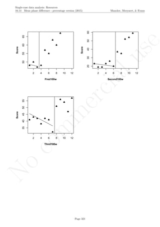
![No
com
m
ercialuse
Single-case data analysis: Resources
16.14 Mean phase difference - percentage version (2015) Manolov, Moeyaert, & Evans
# Copy and paste the rest of the code in the R console
# Whole number function
# Graphical representation of the raw outcome for each tier
par(mfrow=c(2,2))
stripchart(results,vertical=TRUE,ylab="MPD",main="Variability")
points(one_ES,pch=43, col="red",cex=3)
# Plot: tiers against weights (for each tier in the MBD)
plot(tier.weights,results,ylab="MPD",main="Effect size related to weight?")
abline(h=one_ES,col="red")
# Graphical representation of the percentage outcome for each tier
stripchart(stdresults,vertical=TRUE,ylab="MPD percentage",main="Variability")
points(one_stdES,pch=43, col="red",cex=3)
# Plot: tiers against weights (for each tier in the MBD)
plot(tier.weights,stdresults,ylab="MPD percentage",
main="Effect size related to weight?")
abline(h=one_stdES,col="red")
############
# Organize output: raw results
precols <- tiers+2
pretabla <- 1:(2*precols)
dim(pretabla) <- c(2,precols)
pretabla[1,(1:2)] <- c("Id", "Raw MPD")
for (i in 1:tiers)
pretabla[1,(2+i)] <- paste("Tier",i)
pretabla[2,1] <- Data.Id
pretabla[2,2] <- round(one_ES,digits=3)
for (i in 1:tiers)
pretabla[2,(2+i)] <- round(results[i],digits=3)
# Organize results: Percentage results
columns <- tiers+3
tabla <- 1:(2*columns)
dim(tabla) <- c(2,columns)
tabla[1,(1:3)] <- c("Id", "ES", "weight")
for (i in 1:tiers)
tabla[1,(3+i)] <- paste("Tier",i)
tabla[2,1] <- Data.Id
tabla[2,2] <- round(one_stdES,digits=3)
tabla[2,3] <- round(weight_std,digits=3)
for (i in 1:tiers)
tabla[2,(3+i)] <- round(stdresults[i],digits=3)
# Print both tables
print("Results summary: Raw MPD"); print(pretabla,quote=FALSE)
print("Results summary for meta-analysis"); print(tabla,quote=FALSE)
Second part of the code ends here. Default output of the code below:
Page 322](https://image.slidesharecdn.com/635a0af9-e378-45de-b512-1e1e88e419b8-160210073243/85/Tutorial-326-320.jpg)
![No
com
m
ercialuse
Single-case data analysis: Resources
16.14 Mean phase difference - percentage version (2015) Manolov, Moeyaert, & Evans
152025
Variability
MPD
+
10.0 10.5 11.0 11.5 12.0
152025
Effect size related to weight?
tier.weights
MPD
4080120160
Variability
MPDpercentage
+
10.0 10.5 11.0 11.5 12.0
4080120160
Effect size related to weight?
tier.weights
MPDpercentage
## [1] "Results summary: Raw MPD"
## [,1] [,2] [,3] [,4] [,5]
## [1,] Id Raw MPD Tier 1 Tier 2 Tier 3
## [2,] 21.298 12.583 29.2 21
## [1] "Results summary for meta-analysis"
## [,1] [,2] [,3] [,4] [,5] [,6]
## [1,] Id ES weight Tier 1 Tier 2 Tier 3
## [2,] 87.816 33.54 27.772 163.297 66.456
Return to main text in the Tutorial about the modified version of the Mean phase difference: section 6.8.
Page 323](https://image.slidesharecdn.com/635a0af9-e378-45de-b512-1e1e88e419b8-160210073243/85/Tutorial-327-320.jpg)

![No
com
m
ercialuse
Single-case data analysis: Resources
16.15 Mean phase difference - standardized version (2015) Manolov, Moeyaert, & Evans
## 3 Third100w 10 1 54
## 3 Third100w 11 1 47
## 3 Third100w 12 1 57
# Copy and paste the following code in the R console
# Whole number function
# Whole number function
is.wholenumber<- function(x, tol=.Machine$double.eps^0.5) abs(x-round(x)) < tol
# Function for computing MPD, its standardized-version, and mean square error
mpd <- function(baseline,treatment)
{
# Obtain phase length
n_a <- length(baseline)
n_b <- length(treatment)
meanA <- mean(baseline)
# Estimate baseline trend
base_diff <- rep(0,(n_a-1))
for (i in 1:(n_a-1))
base_diff[i] <- baseline[i+1] - baseline[i]
trendA <- mean(base_diff)
# Predict baseline data
baseline_pred <- rep(0,n_a)
midX <- median(c(1:n_a))
midY <- median(baseline)
is.wholenumber <- function(x, tol = .Machine$double.eps^0.5) abs(x - round(x)) < tol
if (is.wholenumber(midX))
{
baseline_pred[midX] <- midY
for (i in (midX-1):1) baseline_pred[i] <- baseline_pred[i+1] - trendA
for (i in (midX+1):n_a) baseline_pred[i] <- baseline_pred[i-1] + trendA
}
if (!is.wholenumber(midX))
{
baseline_pred[midX-0.5] <- midY-(0.5*trendA)
baseline_pred[midX+0.5] <- midY+(0.5*trendA)
for (i in (midX-1.5):1) baseline_pred[i] <- baseline_pred[i+1] - trendA
for (i in (midX+1.5):n_a) baseline_pred[i] <- baseline_pred[i-1] + trendA
}
# Project baseline trend to the treatment phase
treatment_pred <- rep(0,n_b)
treatment_pred[1] <- baseline_pred[n_a] + trendA
for (i in 2:n_b)
treatment_pred[i] <- treatment_pred[i-1]+ trendA
diff_absolute <- rep(0,n_b)
Page 325](https://image.slidesharecdn.com/635a0af9-e378-45de-b512-1e1e88e419b8-160210073243/85/Tutorial-329-320.jpg)
![No
com
m
ercialuse
Single-case data analysis: Resources
16.15 Mean phase difference - standardized version (2015) Manolov, Moeyaert, & Evans
for (i in 1:n_b)
{
diff_absolute[i] <- treatment[i]-treatment_pred[i]
}
mpd_value <- mean(diff_absolute)
mpd_relative <- mpd_value/sd(baseline)
list(mpd_value,mpd_relative,baseline_pred)
}
##########################
# Create the objects necessary for the calculations and the graphs
# Dimensions of the data set
tiers <- max(MBD$Tier)
max.length <- max(MBD$Time)
max.score <- max(MBD$Score)
min.score <- min(MBD$Score)
# Vectors for keeping the main results
# Series lengths per tier
obs <- rep(0,tiers)
# Raw MPD effect sizes per tier
results <- rep(0,tiers)
# Weights per tier
tier.weights <- rep(0,tiers)
# Standardized MPD results per tier
stdresults <- rep(0,tiers)
# Obtain the values calling the MPD function
for (i in 1:tiers)
{
tempo <- subset(MBD,Tier==i)
# Number of observations for the tier
obs[i] <- max(tempo$Time)
# Data corresponding to phase A
Atemp <- subset(tempo,Phase==0)
Aphase <- Atemp$Score
# Data corresponding to phase B
Btemp <- subset(tempo,Phase==1)
Bphase <- Btemp$Score
# Obtain the MPD
results[i] <- mpd(Aphase,Bphase)[[1]]
# Obtain the weight for the MPD
tier.weights[i] <- obs[i]
# Obtain the standardized-version of the MPD
stdresults[i] <- mpd(Aphase,Bphase)[[2]]
}
# Obtain the weighted average: single effect size per study
one_ES_num <- 0
for (i in 1:tiers)
one_ES_num <- one_ES_num + results[i]*tier.weights[i]
one_ES_den <- sum(tier.weights)
one_ES <- one_ES_num / one_ES_den
Page 326](https://image.slidesharecdn.com/635a0af9-e378-45de-b512-1e1e88e419b8-160210073243/85/Tutorial-330-320.jpg)
![No
com
m
ercialuse
Single-case data analysis: Resources
16.15 Mean phase difference - standardized version (2015) Manolov, Moeyaert, & Evans
# Obtain the weight of the single effect size - it's a weight for the meta-analysis
# Weight 1: series length
weight <- sum(obs)
# Obtain the standardized-version of the MPD values for each tier
# Obtain the standardized-version of the weighted average
one_stdES_num <- 0
one_stdES_den <- 0
for (i in 1:tiers)
if (stdresults[i]!=Inf)
{
one_stdES_num<- one_stdES_num + stdresults[i]*tier.weights[i]
one_stdES_den<- one_stdES_den + tier.weights[i]
}
one_stdES <- one_stdES_num / one_stdES_den
############
# Graphical representation of the data & the fitted baseline trend
if (tiers%%2==0) rows <- tiers/2 else rows <- (tiers+1)/2
par(mfrow=c(rows,2))
for (i in 1:tiers)
{
tempo <- subset(MBD,Tier==i)
# Number of observations for the tier
obs[i] <- max(tempo$Time)
# Data corresponding to phase A
Atemp <- subset(tempo,Phase==0)
Aphase <- Atemp$Score
# Data corresponding to phase B
Btemp <- subset(tempo,Phase==1)
Bphase <- Btemp$Score
# Obtain the predicted baseline
Atrend <- mpd(Aphase,Bphase)[[3]]
# Represent graphically
ABphase <- c(Aphase,Bphase)
indep <- 1:length(ABphase)
ymin <- min(min(Atrend),min(ABphase))
ymax <- max(max(Atrend),max(ABphase))
plot(indep,ABphase, xlim=c(1,max.length),
ylim=c(ymin,ymax), xlab=tempo$Id[1], ylab="Score", font.lab=2)
limiter <- length(Aphase)+0.5
abline(v=limiter)
lines(indep[1:length(Aphase)],Atrend[1:length(Aphase)])
points(indep,ABphase, pch=24, bg="black")
}
Page 327](https://image.slidesharecdn.com/635a0af9-e378-45de-b512-1e1e88e419b8-160210073243/85/Tutorial-331-320.jpg)
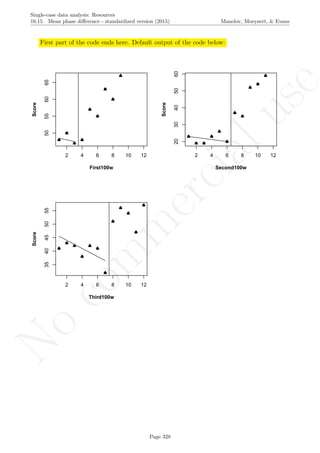
![No
com
m
ercialuse
Single-case data analysis: Resources
16.15 Mean phase difference - standardized version (2015) Manolov, Moeyaert, & Evans
# Copy and paste the rest of the code in the R console
# Whole number function
# Graphical representation of the raw outcome for each tier
par(mfrow=c(2,2))
stripchart(results,vertical=TRUE,ylab="MPD",main="Variability")
points(one_ES,pch=43, col="red",cex=3)
# Plot: tiers against weights (for each tier in the MBD)
plot(tier.weights,results,ylab="MPD",main="Effect size related to weight?")
abline(h=one_ES,col="red")
# Graphical representation of the standardized outcome for each tier
stripchart(stdresults,vertical=TRUE,ylab="MPD standardized",main="Variability")
points(one_stdES,pch=43, col="red",cex=3)
# Plot: tiers against weights (for each tier in the MBD)
plot(tier.weights,stdresults,ylab="MPD standardized",
main="Effect size related to weight?")
abline(h=one_stdES,col="red")
############
# Organize output: raw results
precols <- tiers+2
pretabla <- 1:(2*precols)
dim(pretabla) <- c(2,precols)
pretabla[1,(1:2)] <- c("Id", "Raw MPD")
for (i in 1:tiers)
pretabla[1,(2+i)] <- paste("Tier",i)
pretabla[2,1] <- Data.Id
pretabla[2,2] <- round(one_ES,digits=3)
for (i in 1:tiers)
pretabla[2,(2+i)] <- round(results[i],digits=3)
# Organize results: Percentage results
columns <- tiers+3
tabla <- 1:(2*columns)
dim(tabla) <- c(2,columns)
tabla[1,(1:3)] <- c("Id", "ES", "weight")
for (i in 1:tiers)
tabla[1,(3+i)] <- paste("Tier",i)
tabla[2,1] <- Data.Id
tabla[2,2] <- round(one_stdES,digits=3)
tabla[2,3] <- round(weight,digits=3)
for (i in 1:tiers)
tabla[2,(3+i)] <- round(stdresults[i],digits=3)
# Print both tables
print("Results summary: Raw MPD"); print(pretabla,quote=FALSE)
print("Results summary for meta-analysis"); print(tabla,quote=FALSE)
Second part of the code ends here. Default output of the code below:
Page 329](https://image.slidesharecdn.com/635a0af9-e378-45de-b512-1e1e88e419b8-160210073243/85/Tutorial-333-320.jpg)
![No
com
m
ercialuse
Single-case data analysis: Resources
16.15 Mean phase difference - standardized version (2015) Manolov, Moeyaert, & Evans
152025
Variability
MPD
+
9.0 9.5 10.0 11.0 12.0
152025
Effect size related to weight?
tier.weights
MPD
678910
Variability
MPDstandardized
+
9.0 9.5 10.0 11.0 12.0
678910
Effect size related to weight?
tier.weights
MPDstandardized
## [1] "Results summary: Raw MPD"
## [,1] [,2] [,3] [,4] [,5]
## [1,] Id Raw MPD Tier 1 Tier 2 Tier 3
## [2,] 21.452 12.583 29.2 21
## [1] "Results summary for meta-analysis"
## [,1] [,2] [,3] [,4] [,5] [,6]
## [1,] Id ES weight Tier 1 Tier 2 Tier 3
## [2,] 7.965 32 8.238 10.411 5.519
Return to main text in the Tutorial about the modified version of Mean phase difference: section ??.
Page 330](https://image.slidesharecdn.com/635a0af9-e378-45de-b512-1e1e88e419b8-160210073243/85/Tutorial-334-320.jpg)
![No
com
m
ercialuse
Single-case data analysis: Resources
16.16 Slope and level change - original version (2010) Manolov, Moeyaert, & Evans
16.16 Slope and level change - original version (2010)
This code refers to the origina version of the SLC, as described in Behavior Modification in 2010, comparing, on
the one hand, baseline trend with treatment phase trend and, on the other hand, baseline level with treatment
phase level. The differences are expressed in absolute raw terms (i.e., in the same measurement units as the
target behavior).
# Input data: values in () separated by commas
# n_a denotes number of baseline phase measurements
info <- c(10,9,9,8,7,8,8,7,7,6,4,3,2,1,1,2,1,1,0,0)
n_a <- 10
# Copy and paste the rest of the code in the R console
# Initial data manipulations
slength <- length(info)
n_b <- slength-n_a
phaseA <- info[1:n_a]
phaseB <- info[(n_a+1):slength]
# Estimate phase A trend
phaseAdiff <- c(1:(n_a-1))
for (iter in 1:(n_a-1))
phaseAdiff[iter] <- phaseA[iter+1] - phaseA[iter]
trendA <- mean(phaseAdiff)
# Remove phase A trend from the whole data series
phaseAdet <- c(1:n_a)
for (timeA in 1:n_a)
phaseAdet[timeA] <- phaseA[timeA] - trendA * timeA
phaseBdet <- c(1:n_b)
for (timeB in 1:n_b)
phaseBdet[timeB] <- phaseB[timeB] - trendA * (timeB+n_a)
# Compute the slope change estimate
phaseBdiff <- c(1:(n_b-1))
for (iter in 1:(n_b-1))
phaseBdiff[iter] <- phaseBdet[iter+1] - phaseBdet[iter]
trendB <- mean(phaseBdiff)
# Compute the level change estimate
phaseBddet <- c(1:n_b)
for (timeB in 1:n_b)
phaseBddet[timeB] <- phaseBdet[timeB] - trendB * (timeB-1)
level <- mean(phaseBddet) - mean(phaseAdet)
# Additional calculations for the graph
A_pred <- rep(0,n_a)
A_pred[1] <- info[1]
for (i in 2:n_a)
A_pred[i] <- A_pred[i-1]+trendA
Page 331](https://image.slidesharecdn.com/635a0af9-e378-45de-b512-1e1e88e419b8-160210073243/85/Tutorial-335-320.jpg)
![No
com
m
ercialuse
Single-case data analysis: Resources
16.16 Slope and level change - original version (2010) Manolov, Moeyaert, & Evans
B_pred <- rep(0,n_b)
B_pred[1] <- A_pred[n_a] + trendA
for (i in 2:n_b)
B_pred[i] <- B_pred[i-1]+trendA
A_pred_det <- rep(phaseAdet[1],n_a)
B_slope <- rep(0,n_b)
B_slope[1] <- phaseBdet[1]
for (i in 2:n_b)
B_slope[i] <- B_slope[i-1]+trendB
######################################################################
# Represent graphically actual and detrended data
time <- c(1:slength)
par(mfrow=c(3,1))
plot(time,info, xlim=c(1,slength), ylim=c((min(info)-1),(max(info)+1)),
xlab="Measurement time", ylab="Variable of interest", font.lab=2)
abline(v=(n_a+0.5))
lines(time[1:n_a],info[1:n_a])
lines(time[1:n_a],A_pred[1:n_a],lty="dashed",col="green")
lines(time[(n_a+1):slength],info[(n_a+1):slength])
lines(time[(n_a+1):slength],B_pred,lty="dashed",col="red")
axis(side=1, at=seq(0,slength,1),labels=TRUE, font=2)
#axis(side=2, at=seq((min(info)-1),(max(info)+1),2),labels=TRUE, font=2)
points(time, info, pch=24, bg="black")
title (main="Original data")
transf <- c(phaseAdet,phaseBdet)
title(sub=list(paste("Baseline trend =", round(trendA,2)),col="darkgreen"))
plot(time,transf, xlim=c(1,slength), ylim=c((min(transf)-1),(max(transf)+1)),
xlab="Measurement time", ylab="Variable of interest", font.lab=2)
abline(v=(n_a+0.5))
lines(time[1:n_a],transf[1:n_a])
lines(time[(n_a+1):slength],transf[(n_a+1):slength])
lines(time[(n_a+1):slength],B_slope,lty="dashed",col="red")
lines(time[1:n_a],A_pred_det[1:n_a],lty="dashed",col="green")
axis(side=1, at=seq(0,slength,1),labels=TRUE, font=2)
#axis(side=2, at=seq((min(transf)-1),(max(transf)+1),2),labels=TRUE, font=2)
points(time, transf, pch=24, bg="black")
title (main="Detrended data")
title (sub=list(paste("Change in slope =", round(trendB,2)),col="red"))
retransf <- c(phaseAdet,phaseBddet)
plot(time,retransf, xlim=c(1,slength), ylim=c((min(retransf)-1),(max(retransf)+1)),
xlab="Measurement time", ylab="Variable of interest", font.lab=2)
abline(v=(n_a+0.5))
lines(time[1:n_a],retransf[1:n_a])
lines(time[1:n_a],rep(mean(phaseAdet),n_a),col="blue",lty="dashed")
lines(time[(n_a+1):slength],retransf[(n_a+1):slength])
lines(time[(n_a+1):slength],rep(mean(phaseBddet),n_b),col="blue",lty="dashed")
axis(side=1, at=seq(0,slength,1),labels=TRUE, font=2)
#axis(side=2, at=seq((min(transf)-1),(max(transf)+1),2),labels=TRUE, font=2)
points(time, retransf, pch=24, bg="black")
title (main="Detrended data with no phase B slope")
title (sub=list(paste("Net change in level =", round(level,2)),col="blue"))
Page 332](https://image.slidesharecdn.com/635a0af9-e378-45de-b512-1e1e88e419b8-160210073243/85/Tutorial-336-320.jpg)

![No
com
m
ercialuse
Single-case data analysis: Resources
16.16 Slope and level change - original version (2010) Manolov, Moeyaert, & Evans
Code ends here. Default output of the code below:
5 10 15 20
02468
Measurement time
Variableofinterest
1 2 3 4 5 6 7 8 9 10 11 12 13 14 15 16 17 18 19 20
Original data
Baseline trend = −0.44
5 10 15 20
678911
Measurement time
Variableofinterest
1 2 3 4 5 6 7 8 9 10 11 12 13 14 15 16 17 18 19 20
Detrended data
Change in slope = 0
5 10 15 20
678911
Measurement time
Variableofinterest
1 2 3 4 5 6 7 8 9 10 11 12 13 14 15 16 17 18 19 20
Detrended data with no phase B slope
Net change in level = −1.96
## [1] "Baseline trend estimate = "
## [1] -0.44
## [1] "Slope change estimate = "
## [1] 0
## [1] "Net level change estimate = "
## [1] -1.96
Return to main text in the Tutorial about the original version of the Slope and level change: section 6.9.
Page 334](https://image.slidesharecdn.com/635a0af9-e378-45de-b512-1e1e88e419b8-160210073243/85/Tutorial-338-320.jpg)

![No
com
m
ercialuse
Single-case data analysis: Resources
16.17 Slope and level change - percentage version (2015) Manolov, Moeyaert, & Evans
# Copy and paste the following code in the R console
# Function for computing SLC, its percentage-version, and mean square error
slc <- function(baseline,treatment)
{
phaseA <- baseline
phaseB <- treatment
n_b <- length(phaseB)
n_a <- length(phaseA)
slength <- n_a+n_b
# Estimate phase A trend
phaseAdiff <- c(1:(n_a-1))
for (iter in 1:(n_a-1))
phaseAdiff[iter] <- phaseA[iter+1] - phaseA[iter]
trendA <- mean(phaseAdiff)
# Remove phase A trend from the whole data series
phaseAdet <- c(1:n_a)
for (timeA in 1:n_a)
phaseAdet[timeA] <- phaseA[timeA] - trendA * timeA
phaseBdet <- c(1:n_b)
for (timeB in 1:n_b)
phaseBdet[timeB] <- phaseB[timeB] - trendA * (timeB+n_a)
# Compute the slope change estimate
phaseBdiff <- c(1:(n_b-1))
for (iter in 1:(n_b-1))
phaseBdiff[iter] <- phaseBdet[iter+1] - phaseBdet[iter]
trendB <- mean(phaseBdiff)
# Compute the level change estimate
phaseBddet <- c(1:n_b)
for (timeB in 1:n_b)
phaseBddet[timeB] <- phaseBdet[timeB] - trendB * (timeB-1)
level <- mean(phaseBddet) - mean(phaseAdet)
# Relative index
slope_relative <- (trendB/abs(trendA))*100
level_relative <- (level/mean(phaseAdet))*100
# Predict baseline data
baseline_pred <- rep(0,n_a)
midX <- median(c(1:n_a))
midY <- median(baseline)
is.wholenumber<- function(x, tol=.Machine$double.eps^0.5) abs(x-round(x)) < tol
if (is.wholenumber(midX))
{
baseline_pred[midX] <- midY
for (i in (midX-1):1) baseline_pred[i] <- baseline_pred[i+1] - trendA
for (i in (midX+1):n_a) baseline_pred[i] <- baseline_pred[i-1] + trendA
}
Page 336](https://image.slidesharecdn.com/635a0af9-e378-45de-b512-1e1e88e419b8-160210073243/85/Tutorial-340-320.jpg)
![No
com
m
ercialuse
Single-case data analysis: Resources
16.17 Slope and level change - percentage version (2015) Manolov, Moeyaert, & Evans
if (!is.wholenumber(midX))
{
baseline_pred[midX-0.5] <- midY-(0.5*trendA)
baseline_pred[midX+0.5] <- midY+(0.5*trendA)
for (i in (midX-1.5):1) baseline_pred[i] <- baseline_pred[i+1] - trendA
for (i in (midX+1.5):n_a) baseline_pred[i] <- baseline_pred[i-1] + trendA
}
# Compute the residual (MSE): difference between actual and predicted baseline data
residual <- 0
for (i in 1:n_a)
residual <- residual + (baseline[i]-baseline_pred[i])*(baseline[i]-baseline_pred[i])
residual_mse <- residual/n_a
list(trendB,level,residual_mse,slope_relative,level_relative,baseline_pred)
}
##########################
# Create the objects necessary for the calculations and the graphs
# Dimensions of the data set
tiers <- max(MBD$Tier)
max.length <- max(MBD$Time)
max.score <- max(MBD$Score)
min.score <- min(MBD$Score)
# Vectors for keeping the main results
# Series lengths per tier
obs <- rep(0,tiers)
# Raw SLC effect sizes per tier
results_sc <- rep(0,tiers)
results_lc <- rep(0,tiers)
# Weights per tier
tier.weights_mse <- rep(0,tiers)
tier.weights <- rep(0,tiers)
# Percentage SLC results per tier
stdresults_sc <- rep(0,tiers)
stdresults_lc <- rep(0,tiers)
# Obtain the values calling the SLC function
for (i in 1:tiers)
{
tempo <- subset(MBD,Tier==i)
# Number of observations for the tier
obs[i] <- max(tempo$Time)
# Data corresponding to phase A
Atemp <- subset(tempo,Phase==0)
Aphase <- Atemp$Score
# Data corresponding to phase B
Btemp <- subset(tempo,Phase==1)
Bphase <- Btemp$Score
# Obtain the SLC
results_sc[i] <- slc(Aphase,Bphase)[[1]]
results_lc[i] <- slc(Aphase,Bphase)[[2]]
Page 337](https://image.slidesharecdn.com/635a0af9-e378-45de-b512-1e1e88e419b8-160210073243/85/Tutorial-341-320.jpg)
![No
com
m
ercialuse
Single-case data analysis: Resources
16.17 Slope and level change - percentage version (2015) Manolov, Moeyaert, & Evans
# Obtain the weight for the SLC
tier.weights_mse[i] <- slc(Aphase,Bphase)[[3]]
# Obtain the weight for the MPD
if (tier.weights_mse[i] != 0) tier.weights[i] <-
obs[i]+1/tier.weights_mse[i]
tier.w.sorted <- sort(tier.weights_mse,decreasing = TRUE)
for (j in 1:tiers) if (tier.w.sorted[j] !=0)
tier.w.min <- tier.w.sorted[j]
if (tier.weights_mse[i] == 0)
tier.weights[i] <- obs[i]+1/tier.w.min
# Obtain the percentage-version of the SLC
stdresults_sc[i] <- slc(Aphase,Bphase)[[4]]
stdresults_lc[i] <- slc(Aphase,Bphase)[[5]]
}
# Obtain the weighted average: single effect size per study
one_sc_num <- 0
for (i in 1:tiers)
one_sc_num <- one_sc_num + results_sc[i]*tier.weights[i]
one_sc_den <- sum(tier.weights)
one_sc <- one_sc_num / one_sc_den
one_lc_num <- 0
for (i in 1:tiers)
one_lc_num <- one_lc_num + results_lc[i]*tier.weights[i]
one_lc_den <- sum(tier.weights)
one_lc <- one_lc_num / one_lc_den
# Obtain the weight of the single effect size -
# it's a weight for the meta-analysis
# Weight 1: series length
weight1 <- sum(obs)
# Obtain the percentage-version of the SLC values for each tier
# Obtain the percentage-version of the weighted average
one_stdSC_num <- 0
one_stdSC_den <- 0
infs <- 0
for (i in 1:tiers)
if ((abs(stdresults_sc[i]))!=Inf && is.nan(stdresults_sc[i])==FALSE)
{ one_stdSC_num <- one_stdSC_num + stdresults_sc[i]*tier.weights[i]
one_stdSC_den <- one_stdSC_den + tier.weights[i]}
one_stdSC <- one_stdSC_num / one_stdSC_den
one_stdLC_num <- 0
for (i in 1:tiers)
one_stdLC_num <- one_stdLC_num + stdresults_lc[i]*tier.weights[i]
one_stdLC_den <- sum(tier.weights)
one_stdLC <- one_stdLC_num / one_stdLC_den
# Obtain the weight of the single effect size -
# it's a weight for the meta-analysis
# Weight 1: series length
weight1 <- sum(obs)
variation_sc <- 0
if (tiers == 1) weight2_sc = 1
Page 338](https://image.slidesharecdn.com/635a0af9-e378-45de-b512-1e1e88e419b8-160210073243/85/Tutorial-342-320.jpg)
![No
com
m
ercialuse
Single-case data analysis: Resources
16.17 Slope and level change - percentage version (2015) Manolov, Moeyaert, & Evans
valids_sc <- 0
if (tiers != 1) {
for (i in 1:tiers)
if ((abs(stdresults_sc[i]))!=Inf && is.nan(stdresults_sc[i])==FALSE)
{valids_sc <- valids_sc + 1
variation_sc <- variation_sc + (stdresults_sc[i]-one_stdSC)*
+ (stdresults_sc[i]-one_stdSC)}
# Weight two: variability of the outcomes
coefvar_sc <- (sqrt(variation_sc/valids_sc))/abs(one_stdSC)
weight2_sc <- 1/coefvar_sc
}
# Weight
weight_std_sc <- weight1 + weight2_sc
variation_lc <- 0
if (tiers == 1) weight2_lc = 1
if (tiers != 1) {
for (i in 1:tiers)
variation_lc <- variation_lc + (stdresults_lc[i]-one_stdLC)*
+ (stdresults_lc[i]-one_stdLC)
# Weight two: variability of the outcomes
coefvar_lc <- (sqrt(variation_lc/tiers))/abs(one_stdLC)
weight2_lc <- 1/coefvar_lc
}
# Weight
weight_std_lc <- weight1 + weight2_lc
############
# Graphical representation of the data & the fitted baseline trend
if (tiers%%2==0) rows <- tiers/2 else rows <- (tiers+1)/2
par(mfrow=c(rows,2))
for (i in 1:tiers)
{
tempo <- subset(MBD,Tier==i)
# Number of observations for the tier
obs[i] <- max(tempo$Time)
# Data corresponding to phase A
Atemp <- subset(tempo,Phase==0)
Aphase <- Atemp$Score
# Data corresponding to phase B
Btemp <- subset(tempo,Phase==1)
Bphase <- Btemp$Score
# Obtain the predicted baseline
Atrend <- slc(Aphase,Bphase)[[6]]
# Represent graphically
ABphase <- c(Aphase,Bphase)
indep <- 1:length(ABphase)
ymin <- min(min(Atrend),min(ABphase))
ymax <- max(max(Atrend),max(ABphase))
plot(indep,ABphase, xlim=c(1,max.length), ylim=c(ymin,ymax), xlab=tempo$Id[1], ylab="Score", font.lab
Page 339](https://image.slidesharecdn.com/635a0af9-e378-45de-b512-1e1e88e419b8-160210073243/85/Tutorial-343-320.jpg)
![No
com
m
ercialuse
Single-case data analysis: Resources
16.17 Slope and level change - percentage version (2015) Manolov, Moeyaert, & Evans
limiter <- length(Aphase)+0.5
abline(v=limiter)
lines(indep[1:length(Aphase)],Atrend[1:length(Aphase)])
points(indep,ABphase, pch=24, bg="black")
}
First part of the code ends here. Default output of the code below:
2 4 6 8 10 12
50556065
First100w
Score
2 4 6 8 10 12
2030405060
Second100w
Score
2 4 6 8 10 12
3540455055
Third100w
Score
Page 340](https://image.slidesharecdn.com/635a0af9-e378-45de-b512-1e1e88e419b8-160210073243/85/Tutorial-344-320.jpg)
![No
com
m
ercialuse
Single-case data analysis: Resources
16.17 Slope and level change - percentage version (2015) Manolov, Moeyaert, & Evans
# Copy and paste the rest of the code in the R console
# Whole number function
# Graphical representation of the raw outcome for each tier
par(mfrow=c(2,4))
stripchart(results_sc,vertical=TRUE,ylab="Slope change",
main="Variability")
points(one_sc,pch=43, col="red",cex=3)
# Plot: tiers against weights (for each tier in the MBD)
plot(tier.weights,results_sc,ylab="Slope change",
main="Effect size related to weight?")
abline(h=one_sc,col="red")
stripchart(results_lc,vertical=TRUE,ylab="Level change",
main="Variability")
points(one_lc,pch=43, col="red",cex=3)
# Plot: tiers against weights (for each tier in the MBD)
plot(tier.weights,results_lc,ylab="Level change",
main="Effect size related to weight?")
abline(h=one_lc,col="red")
# Graphical representation of the percentage outcome for each tier
stripchart(stdresults_sc,vertical=TRUE,
ylab="SC percentage",main="Variability")
points(one_stdSC,pch=43, col="red",cex=3)
# Plot: tiers against weights (for each tier in the MBD)
plot(tier.weights,stdresults_sc,ylab="SC percentage",
main="Effect size related to weight?")
abline(h=one_stdSC,col="red")
stripchart(stdresults_lc,vertical=TRUE,
ylab="LC percentage",main="Variability")
points(one_stdLC, pch=43, col="red",cex=3)
# Plot: tiers against weights (for each tier in the MBD)
plot(tier.weights,stdresults_lc,
ylab="LC percentage",main="Effect size related to weight?")
abline(h=one_stdLC,col="red")
############
# Organize output: raw results
precols <- tiers+3
pretabla <- 1:(3*precols)
dim(pretabla) <- c(3,precols)
pretabla[1,(1:3)] <- c("Id", "TypeEffect", "Value")
for (i in 1:tiers)
pretabla[1,(3+i)] <- paste("Tier",i)
pretabla[2,1] <- Data.Id
pretabla[2,2] <- "SlopeChange"
pretabla[2,3] <- round(one_sc,digits=3)
for (i in 1:tiers)
pretabla[2,(3+i)] <- round(results_sc[i],digits=3)
pretabla[3,1] <- Data.Id
pretabla[3,2] <- "LevelChange"
pretabla[3,3] <- round(one_lc,digits=3)
for (i in 1:tiers)
pretabla[3,(3+i)] <- round(results_lc[i],digits=3)
Page 341](https://image.slidesharecdn.com/635a0af9-e378-45de-b512-1e1e88e419b8-160210073243/85/Tutorial-345-320.jpg)
![No
com
m
ercialuse
Single-case data analysis: Resources
16.17 Slope and level change - percentage version (2015) Manolov, Moeyaert, & Evans
# Organize results: Percentage results
columns <- tiers+4
tabla <- 1:(3*columns)
dim(tabla) <- c(3,columns)
tabla[1,(1:4)] <- c("Id", "TypeEffect", "ES", "Weight")
for (i in 1:tiers)
tabla[1,(4+i)] <- paste("Tier",i)
tabla[2,1] <- Data.Id
tabla[2,2] <- "SlopeChange"
tabla[2,3] <- round(one_stdSC,digits=3)
tabla[2,4] <- round(weight_std_sc,digits=3)
for (i in 1:tiers)
tabla[2,(4+i)] <- round(stdresults_sc[i],digits=3)
tabla[3,1] <- Data.Id
tabla[3,2] <- "LevelChange"
tabla[3,3] <- round(one_stdLC,digits=3)
tabla[3,4] <- round(weight_std_lc,digits=3)
for (i in 1:tiers)
tabla[3,(4+i)] <- round(stdresults_lc[i],digits=3)
# Print both tables
print("Results summary: Raw SLC"); print(pretabla,quote=FALSE)
print("Results summary for meta-analysis"); print(tabla,quote=FALSE)
Second part of the code ends here. Default output of the code below:
Page 342](https://image.slidesharecdn.com/635a0af9-e378-45de-b512-1e1e88e419b8-160210073243/85/Tutorial-346-320.jpg)
![No
com
m
ercialuse
Single-case data analysis: Resources
16.17 Slope and level change - percentage version (2015) Manolov, Moeyaert, & Evans
3.03.54.04.55.05.56.0
Variability
Slopechange
+
10.0 11.0 12.0
3.03.54.04.55.05.56.0
Effect size related to weight?
tier.weights
Slopechange
51015
Variability
Levelchange
+
10.0 11.0 12.0
51015
Effect size related to weight?
tier.weights
Levelchange
2004006008001000
Variability
SCpercentage
+
10.0 11.0 12.0
2004006008001000
Effect size related to weight?
tier.weights
SCpercentage
10203040506070
Variability
LCpercentage
+
10.0 11.0 12.0
10203040506070
Effect size related to weight?
tier.weights
LCpercentage
## [1] "Results summary: Raw SLC"
## [,1] [,2] [,3] [,4] [,5] [,6]
## [1,] Id TypeEffect Value Tier 1 Tier 2 Tier 3
## [2,] SlopeChange 4.43 4.3 6.1 3
## [3,] LevelChange 12.072 1.5 16.833 16.143
## [1] "Results summary for meta-analysis"
## [,1] [,2] [,3] [,4] [,5] [,6] [,7]
## [1,] Id TypeEffect ES Weight Tier 1 Tier 2 Tier 3
## [2,] SlopeChange 670.009 33.89 860 1016.667 200
## [3,] LevelChange 37.79 33.363 3.041 70.827 35.202
Return to main text in the Tutorial about the modified version of the Slope and level change: section 6.10.
Page 343](https://image.slidesharecdn.com/635a0af9-e378-45de-b512-1e1e88e419b8-160210073243/85/Tutorial-347-320.jpg)

![No
com
m
ercialuse
Single-case data analysis: Resources
16.18 Slope and level change - standardized version (2015) Manolov, Moeyaert, & Evans
# Copy and paste the following code in the R console
# Function for computing SLC, its standardized-version, and mean square error
slc <- function(baseline,treatment)
{
phaseA <- baseline
phaseB <- treatment
n_b <- length(phaseB)
n_a <- length(phaseA)
slength <- n_a+n_b
# Estimate phase A trend
phaseAdiff <- c(1:(n_a-1))
for (iter in 1:(n_a-1))
phaseAdiff[iter] <- phaseA[iter+1] - phaseA[iter]
trendA <- mean(phaseAdiff)
# Remove phase A trend from the whole data series
phaseAdet <- c(1:n_a)
for (timeA in 1:n_a)
phaseAdet[timeA] <- phaseA[timeA] - trendA * timeA
phaseBdet <- c(1:n_b)
for (timeB in 1:n_b)
phaseBdet[timeB] <- phaseB[timeB] - trendA * (timeB+n_a)
# Compute the slope change estimate
phaseBdiff <- c(1:(n_b-1))
for (iter in 1:(n_b-1))
phaseBdiff[iter] <- phaseBdet[iter+1] - phaseBdet[iter]
trendB <- mean(phaseBdiff)
# Compute the level change estimate
phaseBddet <- c(1:n_b)
for (timeB in 1:n_b)
phaseBddet[timeB] <- phaseBdet[timeB] - trendB * (timeB-1)
level <- mean(phaseBddet) - mean(phaseAdet)
# Relative index
slope_relative <- trendB/sd(baseline)
level_relative <- level/sd(baseline)
# Predict baseline data
baseline_pred <- rep(0,n_a)
midX <- median(c(1:n_a))
midY <- median(baseline)
is.wholenumber <- function(x, tol = .Machine$double.eps^0.5) abs(x - round(x)) < tol
if (is.wholenumber(midX))
{
baseline_pred[midX] <- midY
for (i in (midX-1):1) baseline_pred[i] <- baseline_pred[i+1] - trendA
for (i in (midX+1):n_a) baseline_pred[i] <- baseline_pred[i-1] + trendA
}
Page 345](https://image.slidesharecdn.com/635a0af9-e378-45de-b512-1e1e88e419b8-160210073243/85/Tutorial-349-320.jpg)
![No
com
m
ercialuse
Single-case data analysis: Resources
16.18 Slope and level change - standardized version (2015) Manolov, Moeyaert, & Evans
if (!is.wholenumber(midX))
{
baseline_pred[midX-0.5] <- midY-(0.5*trendA)
baseline_pred[midX+0.5] <- midY+(0.5*trendA)
for (i in (midX-1.5):1) baseline_pred[i] <- baseline_pred[i+1] - trendA
for (i in (midX+1.5):n_a) baseline_pred[i] <- baseline_pred[i-1] + trendA
}
list(trendB,level,slope_relative,level_relative,baseline_pred)
}
##########################
# Create the objects necessary for the calculations and the graphs
# Dimensions of the data set
tiers <- max(MBD$Tier)
max.length <- max(MBD$Time)
max.score <- max(MBD$Score)
min.score <- min(MBD$Score)
# Vectors for keeping the main results
# Series lengths per tier
obs <- rep(0,tiers)
# Raw SLC effect sizes per tier
results_sc <- rep(0,tiers)
results_lc <- rep(0,tiers)
# Weights per tier
tier.weights <- rep(0,tiers)
# Percentage SLC results per tier
stdresults_sc <- rep(0,tiers)
stdresults_lc <- rep(0,tiers)
# Obtain the values calling the SLC function
for (i in 1:tiers)
{
tempo <- subset(MBD,Tier==i)
# Number of observations for the tier
obs[i] <- max(tempo$Time)
# Data corresponding to phase A
Atemp <- subset(tempo,Phase==0)
Aphase <- Atemp$Score
# Data corresponding to phase B
Btemp <- subset(tempo,Phase==1)
Bphase <- Btemp$Score
# Obtain the SLC
results_sc[i] <- slc(Aphase,Bphase)[[1]]
results_lc[i] <- slc(Aphase,Bphase)[[2]]
# Obtain the weight for the SLC
tier.weights[i] <- obs[i]
# Obtain the standardized-version of the SLC
stdresults_sc[i] <- slc(Aphase,Bphase)[[3]]
stdresults_lc[i] <- slc(Aphase,Bphase)[[4]]
}
# Obtain the weighted average: single effect size per study
one_sc_num <- 0
for (i in 1:tiers)
Page 346](https://image.slidesharecdn.com/635a0af9-e378-45de-b512-1e1e88e419b8-160210073243/85/Tutorial-350-320.jpg)
![No
com
m
ercialuse
Single-case data analysis: Resources
16.18 Slope and level change - standardized version (2015) Manolov, Moeyaert, & Evans
one_sc_num <- one_sc_num + results_sc[i]*tier.weights[i]
one_sc_den <- sum(tier.weights)
one_sc <- one_sc_num / one_sc_den
one_lc_num <- 0
for (i in 1:tiers)
one_lc_num <- one_lc_num + results_lc[i]*tier.weights[i]
one_lc_den <- sum(tier.weights)
one_lc <- one_lc_num / one_lc_den
# Obtain the weight of the single effect size - it's a weight for the meta-analysis
# Weight 1: series length
weight <- sum(obs)
# Obtain the standardized-version of the SLC values for each tier
# Obtain the standardized-version of the weighted average
one_stdSC_num <- 0
for (i in 1:tiers)
one_stdSC_num <- one_stdSC_num + stdresults_sc[i]*tier.weights[i]
one_stdSC_den <- sum(tier.weights)
one_stdSC <- one_stdSC_num / one_stdSC_den
one_stdLC_num <- 0
for (i in 1:tiers)
one_stdLC_num <- one_stdLC_num + stdresults_lc[i]*tier.weights[i]
one_stdLC_den <- sum(tier.weights)
one_stdLC <- one_stdLC_num / one_stdLC_den
############
# Graphical representation of the data & the fitted baseline trend
if (tiers%%2==0) rows <- tiers/2 else rows <- (tiers+1)/2
par(mfrow=c(rows,2))
for (i in 1:tiers)
{
tempo <- subset(MBD,Tier==i)
# Number of observations for the tier
obs[i] <- max(tempo$Time)
# Data corresponding to phase A
Atemp <- subset(tempo,Phase==0)
Aphase <- Atemp$Score
# Data corresponding to phase B
Btemp <- subset(tempo,Phase==1)
Bphase <- Btemp$Score
# Obtain the predicted baseline
Atrend <- slc(Aphase,Bphase)[[5]]
# Represent graphically
ABphase <- c(Aphase,Bphase)
indep <- 1:length(ABphase)
ymin <- min(min(Atrend),min(ABphase))
Page 347](https://image.slidesharecdn.com/635a0af9-e378-45de-b512-1e1e88e419b8-160210073243/85/Tutorial-351-320.jpg)
![No
com
m
ercialuse
Single-case data analysis: Resources
16.18 Slope and level change - standardized version (2015) Manolov, Moeyaert, & Evans
ymax <- max(max(Atrend),max(ABphase))
plot(indep,ABphase, xlim=c(1,max.length), ylim=c(ymin,ymax), xlab=tempo$Id[1], ylab="Score", font.lab
limiter <- length(Aphase)+0.5
abline(v=limiter)
lines(indep[1:length(Aphase)],Atrend[1:length(Aphase)])
points(indep,ABphase, pch=24, bg="black")
}
First part of the code ends here. Default output of the code below:
2 4 6 8 10 12
50556065
First100w
Score
2 4 6 8 10 12
2030405060
Second100w
Score
2 4 6 8 10 12
3540455055
Third100w
Score
Page 348](https://image.slidesharecdn.com/635a0af9-e378-45de-b512-1e1e88e419b8-160210073243/85/Tutorial-352-320.jpg)
![No
com
m
ercialuse
Single-case data analysis: Resources
16.18 Slope and level change - standardized version (2015) Manolov, Moeyaert, & Evans
# Copy and paste the rest of the code in the R console
# Graphical representation of the raw outcome for each tier
par(mfrow=c(2,4))
stripchart(results_sc,vertical=TRUE,ylab="Slope change",
main="Variability")
points(one_sc,pch=43, col="red",cex=3)
# Plot: tiers against weights (for each tier in the MBD)
plot(tier.weights,results_sc,ylab="Slope change",
main="Effect size related to weight?")
abline(h=one_sc,col="red")
stripchart(results_lc,vertical=TRUE,ylab="Level change",
main="Variability")
points(one_lc,pch=43, col="red",cex=3)
# Plot: tiers against weights (for each tier in the MBD)
plot(tier.weights,results_lc,ylab="Level change",
main="Effect size related to weight?")
abline(h=one_lc,col="red")
# Graphical representation of the standardized outcome for each tier
stripchart(stdresults_sc,vertical=TRUE,ylab="SC standardized",
main="Variability")
points(one_stdSC,pch=43, col="red",cex=3)
# Plot: tiers against weights (for each tier in the MBD)
plot(tier.weights,stdresults_sc,ylab="SC standardized",
main="Effect size related to weight?")
abline(h=one_stdSC,col="red")
stripchart(stdresults_lc,vertical=TRUE,ylab="LC standardized",
main="Variability")
points(one_stdLC, pch=43, col="red",cex=3)
# Plot: tiers against weights (for each tier in the MBD)
plot(tier.weights,stdresults_lc,ylab="LC standardized",
main="Effect size related to weight?")
abline(h=one_stdLC,col="red")
############
# Organize output: raw results
precols <- tiers+3
pretabla <- 1:(3*precols)
dim(pretabla) <- c(3,precols)
pretabla[1,(1:3)] <- c("Id", "TypeEffect", "Value")
for (i in 1:tiers)
pretabla[1,(3+i)] <- paste("Tier",i)
pretabla[2,1] <- Data.Id
pretabla[2,2] <- "SlopeChange"
pretabla[2,3] <- round(one_sc,digits=3)
for (i in 1:tiers)
pretabla[2,(3+i)] <- round(results_sc[i],digits=3)
pretabla[3,1] <- Data.Id
pretabla[3,2] <- "LevelChange"
pretabla[3,3] <- round(one_lc,digits=3)
for (i in 1:tiers)
pretabla[3,(3+i)] <- round(results_lc[i],digits=3)
Page 349](https://image.slidesharecdn.com/635a0af9-e378-45de-b512-1e1e88e419b8-160210073243/85/Tutorial-353-320.jpg)
![No
com
m
ercialuse
Single-case data analysis: Resources
16.18 Slope and level change - standardized version (2015) Manolov, Moeyaert, & Evans
# Organize results: Percentage results
columns <- tiers+4
tabla <- 1:(3*columns)
dim(tabla) <- c(3,columns)
tabla[1,(1:4)] <- c("Id", "TypeEffect", "ES", "Weight")
for (i in 1:tiers)
tabla[1,(4+i)] <- paste("Tier",i)
tabla[2,1] <- Data.Id
tabla[2,2] <- "SlopeChange"
tabla[2,3] <- round(one_stdSC,digits=3)
tabla[2,4] <- round(weight,digits=3)
for (i in 1:tiers)
tabla[2,(4+i)] <- round(stdresults_sc[i],digits=3)
tabla[3,1] <- Data.Id
tabla[3,2] <- "LevelChange"
tabla[3,3] <- round(one_stdLC,digits=3)
tabla[3,4] <- round(weight,digits=3)
for (i in 1:tiers)
tabla[3,(4+i)] <- round(stdresults_lc[i],digits=3)
# Print both tables
print("Results summary: Raw SLC"); print(pretabla,quote=FALSE)
print("Results summary for meta-analysis"); print(tabla,quote=FALSE)
Second part of the code ends here. Default output of the code below:
Page 350](https://image.slidesharecdn.com/635a0af9-e378-45de-b512-1e1e88e419b8-160210073243/85/Tutorial-354-320.jpg)
![No
com
m
ercialuse
Single-case data analysis: Resources
16.18 Slope and level change - standardized version (2015) Manolov, Moeyaert, & Evans
3.03.54.04.55.05.56.0
Variability
Slopechange
+
9.0 10.0 11.5
3.03.54.04.55.05.56.0
Effect size related to weight?
tier.weights
Slopechange
51015
Variability
Levelchange
+
9.0 10.0 11.5
51015
Effect size related to weight?
tier.weights
Levelchange
1.01.52.02.5
Variability
SCstandardized
+
9.0 10.0 11.5
1.01.52.02.5
Effect size related to weight?
tier.weights
SCstandardized
123456
Variability
LCstandardized
+
9.0 10.0 11.5
123456
Effect size related to weight?
tier.weights
LCstandardized
## [1] "Results summary: Raw SLC"
## [,1] [,2] [,3] [,4] [,5] [,6]
## [1,] Id TypeEffect Value Tier 1 Tier 2 Tier 3
## [2,] SlopeChange 4.431 4.3 6.1 3
## [3,] LevelChange 12.262 1.5 16.833 16.143
## [1] "Results summary for meta-analysis"
## [,1] [,2] [,3] [,4] [,5] [,6] [,7]
## [1,] Id TypeEffect ES Weight Tier 1 Tier 2 Tier 3
## [2,] SlopeChange 1.835 32 2.815 2.175 0.788
## [3,] LevelChange 3.93 32 0.982 6.002 4.243
Return to main text in the Tutorial about the modified version of the Slope and level change: section 6.10.
Page 351](https://image.slidesharecdn.com/635a0af9-e378-45de-b512-1e1e88e419b8-160210073243/85/Tutorial-355-320.jpg)
![No
com
m
ercialuse
Single-case data analysis: Resources
16.19 Maximal reference approach: Estimating probabilities Manolov, Moeyaert, & Evans
16.19 Maximal reference approach: Estimating probabilities
# Input data: values in () separated by commas
# n_a denotes number of baseline phase measurements
score <- c(3,1,2,2,2,1,1,3,2,4,5,2,0,3,4,6,3,3,4,4,4,6,4,4,4,3,6)
n_a <- 13
# The AB comparison is part of...
## AB design = "AB"
## Reversal/withdrawal design = "ABAB"
## Multiple-baseline design = "MBD"
design <- "AB"
# What's the aim of the intervention: incerase or reduce behavior of interest?
## Increase target behavior = "increase"
## Decrease target behavior = "reduce"
aim <- "increase"
# Which of the following procedure would you like to use?
## Nonoverlap of all pairs = "NAP"
## Percentage of nonoverlapping data = "PND"
## Standardized mean difference using pooled estimate of standard deviation = "Pooled"
## Standardized mean difference using baseline estimate of standard deviation = "Delta"
## Mean phase difference (standardized version, as in Delta) = "MPD"
## Slope and level change (standardized version, as in Delta) = "SLC"
procedure <- "NAP"
# Copy and paste the remaining code in the R console
# Manipulating the data
# Example data set: baseline measurements
baseline <- score[1:n_a]
# Example data set: intervention phase measurements
treatment <- score[(n_a+1):length(score)]
# THE FOLLOWING CODE NEEDS NOT BE CHANGED
# Obtain phase length
n_a <- length(baseline)
n_b <- length(treatment)
# Autocorrelation values:
# Use ShadishSullivan corrected instead of estimating
if (design == "MBD") phi <- 0.321
if (design == "ABAB") phi <- 0.191
if (design == "AB") phi <- 0.752
Page 352](https://image.slidesharecdn.com/635a0af9-e378-45de-b512-1e1e88e419b8-160210073243/85/Tutorial-356-320.jpg)
![No
com
m
ercialuse
Single-case data analysis: Resources
16.19 Maximal reference approach: Estimating probabilities Manolov, Moeyaert, & Evans
##########################################
##########################################
# Procedure MPD
if (procedure == "MPD")
{
# Estimate baseline trend
base_diff <- rep(0,(n_a-1))
for (i in 1:(n_a-1))
base_diff[i] <- baseline[i+1] - baseline[i]
trendA <- mean(base_diff)
# Project baseline trend to the treatment phase
treatment_pred <- rep(0,n_b)
for (i in 1:n_b)
treatment_pred[i] <- baseline[1] + trendA*(n_a+i-1)
# PERFORM THE CALCULATIONS
# Compare the predicted and the actually obtained treatment data
# and obtain the average difference
mpd <- mean(treatment-treatment_pred)
mpd_stdzd <- mpd/sd(baseline)
result1 <- paste("Mean phase difference",round(mpd,digits=2))
result2 <- paste("Mean phase difference; standardized",
round(mpd_stdzd,digits=2))
##################################
# Declare the necessary vectors and their size
nsize <- n_a + n_b
iter <- 1000
# Vectors where the values are to be saved
mpd_arr_norm <- rep(0,iter)
mpd_arr_exp <- rep(0,iter)
mpd_arr_unif <- rep(0,iter)
et <- rep(0,nsize)
####################################
# Iterate with Normal
for (iterate in 1:iter)
{
# Generate error term - phase A1
ut <- rnorm(n=nsize,mean=0,sd=1)
et[1] <- ut[1]
for (i in 2:nsize)
et[i] <- phi*et[i-1] + ut[i]
Page 353](https://image.slidesharecdn.com/635a0af9-e378-45de-b512-1e1e88e419b8-160210073243/85/Tutorial-357-320.jpg)
![No
com
m
ercialuse
Single-case data analysis: Resources
16.19 Maximal reference approach: Estimating probabilities Manolov, Moeyaert, & Evans
# Example data set: baseline measurements
baseline <- et[1:n_a]
# Example data set: intervention phase measurements
# change the values within ()
treatment <- et[(n_a+1):nsize]
# THE FOLLOWING CODE NEEDS NOT BE CHANGED
# Obtain phase length
n_a <- length(baseline)
n_b <- length(treatment)
# Estimate baseline trend
base_diff <- rep(0,(n_a-1))
for (i in 1:(n_a-1))
base_diff[i] <- baseline[i+1] - baseline[i]
trendA <- mean(base_diff)
# Project baseline trend to the treatment phase
treatment_pred <- rep(0,n_b)
for (i in 1:n_b)
treatment_pred[i] <- baseline[1] + trendA*(n_a+i-1)
# PERFORM THE CALCULATIONS
# Compare the predicted and the actually obtained treatment
# data and obtain the average difference
mpd <- mean(treatment-treatment_pred)
mpd_arr_norm[iterate] <- mpd/sd(baseline)
}
#################################
# Iterate with Exponential
for (iterate in 1:iter)
{
# Generate error term - phase A1
ut_temp <- rexp(n=nsize,rate=1)
ut <- ut_temp - 1
et[1] <- ut[1]
for (i in 2:nsize)
et[i] <- phi*et[i-1] + ut[i]
# Example data set: baseline measurements
baseline <- et[1:n_a]
# Example data set:
# intervention phase measurements
treatment <- et[(n_a+1):nsize]
# THE FOLLOWING CODE NEEDS NOT BE CHANGED
# Obtain phase length
n_a <- length(baseline)
n_b <- length(treatment)
# Estimate baseline trend
base_diff <- rep(0,(n_a-1))
Page 354](https://image.slidesharecdn.com/635a0af9-e378-45de-b512-1e1e88e419b8-160210073243/85/Tutorial-358-320.jpg)
![No
com
m
ercialuse
Single-case data analysis: Resources
16.19 Maximal reference approach: Estimating probabilities Manolov, Moeyaert, & Evans
for (i in 1:(n_a-1))
base_diff[i] <- baseline[i+1] - baseline[i]
trendA <- mean(base_diff)
# Project baseline trend to the treatment phase
treatment_pred <- rep(0,n_b)
for (i in 1:n_b)
treatment_pred[i] <- baseline[1] + trendA*(n_a+i-1)
# PERFORM THE CALCULATIONS
# Compare the predicted and the actually obtained treatment data
# and obtain the average difference
mpd <- mean(treatment-treatment_pred)
mpd_arr_exp[iterate] <- mpd/sd(baseline)
}
##############################
# Iterate with Uniform
for (iterate in 1:iter)
{
# Generate error term - phase A1
ut <- runif(n=nsize,min=-1.7320508075688773,
max=1.7320508075688773)
et[1] <- ut[1]
for (i in 2:nsize)
et[i] <- phi*et[i-1] + ut[i]
# Example data set: baseline measurements
baseline <- et[1:n_a]
# Example data set: intervention phase measurements
treatment <- et[(n_a+1):nsize]
# THE FOLLOWING CODE NEEDS NOT BE CHANGED
# Obtain phase length
n_a <- length(baseline)
n_b <- length(treatment)
# Estimate baseline trend
base_diff <- rep(0,(n_a-1))
for (i in 1:(n_a-1))
base_diff[i] <- baseline[i+1] - baseline[i]
trendA <- mean(base_diff)
# Project baseline trend to the treatment phase
treatment_pred <- rep(0,n_b)
for (i in 1:n_b)
treatment_pred[i] <- baseline[1] + trendA*(n_a+i-1)
# PERFORM THE CALCULATIONS
# Compare the predicted and the actually obtained
# treatment data and obtain the average difference
mpd <- mean(treatment-treatment_pred)
mpd_arr_unif[iterate] <- mpd/sd(baseline)
}
############################
Page 355](https://image.slidesharecdn.com/635a0af9-e378-45de-b512-1e1e88e419b8-160210073243/85/Tutorial-359-320.jpg)
![No
com
m
ercialuse
Single-case data analysis: Resources
16.19 Maximal reference approach: Estimating probabilities Manolov, Moeyaert, & Evans
mpd_norm_sorted <- sort(mpd_arr_norm)
mpd_exp_sorted <- sort(mpd_arr_exp)
mpd_unif_sorted <- sort(mpd_arr_unif)
# According to the aim
if (aim == "increase")
{
reference.05 <- max(mpd_norm_sorted[950],
mpd_exp_sorted[950],mpd_unif_sorted[950])
reference.10 <- max(mpd_norm_sorted[900],
mpd_exp_sorted[900],mpd_unif_sorted[900])
reference.25 <- max(mpd_norm_sorted[750],
mpd_exp_sorted[750],mpd_unif_sorted[750])
reference.50 <- max(mpd_norm_sorted[500],
mpd_exp_sorted[500],mpd_unif_sorted[500])
# Assess effect
if (mpd_stdzd >= reference.05) result3 <-
"Probability of the effect observed, if actually null: p <= .05"
if ( (mpd_stdzd < reference.05) && (mpd_stdzd >= reference.10) ) result3 <-
"Probability of the effect observed, if actually null: .05 < p <= .10"
if ( (mpd_stdzd < reference.10) && (mpd_stdzd >= reference.25) ) result3 <-
"Probability of the effect observed, if actually null: .10 < p <= .25"
if ( (mpd_stdzd < reference.25) && (mpd_stdzd >= reference.50) ) result3 <-
"Probability of the effect observed, if actually null: .25 < p <= .50"
if (mpd_stdzd < reference.50) result3 <-
"Probability of the effect observed, if actually null: p > .50"
}
if (aim == "reduce")
{
reference.05 <- min(mpd_norm_sorted[50],
mpd_exp_sorted[50],mpd_unif_sorted[50])
reference.10 <- min(mpd_norm_sorted[100],
mpd_exp_sorted[100],mpd_unif_sorted[100])
reference.25 <- min(mpd_norm_sorted[250],
mpd_exp_sorted[250],mpd_unif_sorted[250])
reference.50 <- min(mpd_norm_sorted[500],
mpd_exp_sorted[500],mpd_unif_sorted[500])
# Assess effect
if (mpd_stdzd <= reference.05) result3 <-
"Probability of the effect observed, if actually null: p <= .05"
if ( (mpd_stdzd > reference.05) && (mpd_stdzd <= reference.10) ) result3 <-
"Probability of the effect observed, if actually null: .05 < p <= .10"
if ( (mpd_stdzd > reference.10) && (mpd_stdzd <= reference.25) ) result3 <-
"Probability of the effect observed, if actually null: .10 < p <= .25"
if ( (mpd_stdzd > reference.25) && (mpd_stdzd <= reference.50) ) result3 <-
"Probability of the effect observed, if actually null: .25 < p <= .50"
if (mpd_stdzd > reference.50) result3 <-
"Probability of the effect observed, if actually null: p > .50"
}
}
############################################
Page 356](https://image.slidesharecdn.com/635a0af9-e378-45de-b512-1e1e88e419b8-160210073243/85/Tutorial-360-320.jpg)
![No
com
m
ercialuse
Single-case data analysis: Resources
16.19 Maximal reference approach: Estimating probabilities Manolov, Moeyaert, & Evans
############################################
# Procedure NAP
if (procedure == "NAP")
{
# Compute index for actual data (example NAP)
# Apply NAP
slength <- n_a + n_b
phaseA <- baseline
phaseB <- treatment
# Compute overlaps
complete <- 0
half <- 0
if (aim == "increase")
{
for (iter1 in 1:n_a)
for (iter2 in 1:n_b)
{if (phaseA[iter1] > phaseB[iter2]) complete <- complete + 1;
if (phaseA[iter1] == phaseB[iter2]) half <- half + 1}
# Compute and print corrected NAP
overlapping <- complete + (half/2)
nap_actual <- ((n_a*n_b - overlapping) / (n_a*n_b))*100
}
if (aim == "reduce")
{
for (iter1 in 1:n_a)
for (iter2 in 1:n_b)
{if (phaseA[iter1] < phaseB[iter2]) complete <- complete + 1;
if (phaseA[iter1] == phaseB[iter2]) half <- half + 1}
# Compute and print corrected NAP
overlapping <- complete + (half/2)
nap_actual <- ((n_a*n_b - overlapping) / (n_a*n_b))*100
}
result1 <-
paste("Overlaps and ties",overlapping)
result2 <-
paste("Nonoverlap of all pairs", round(nap_actual, digits=2))
####################################################
# Declare the necessary vectors and their size
nsize <- n_a + n_b
iter <- 1000
# Vectors where the values are to be saved
nap_arr_norm <- rep(0,iter)
nap_arr_exp <- rep(0,iter)
nap_arr_unif <- rep(0,iter)
et <- rep(0,nsize)
Page 357](https://image.slidesharecdn.com/635a0af9-e378-45de-b512-1e1e88e419b8-160210073243/85/Tutorial-361-320.jpg)
![No
com
m
ercialuse
Single-case data analysis: Resources
16.19 Maximal reference approach: Estimating probabilities Manolov, Moeyaert, & Evans
###################################################
# Iterate with Normal
for (iterate in 1:iter)
{
# Generate error term - phase A1
ut <- rnorm(n=nsize,mean=0,sd=1)
et[1] <- ut[1]
for (i in 2:nsize)
et[i] <- phi*et[i-1] + ut[i]
# Apply NAP
slength <- length(et)
phaseA <- et[1:n_a]
phaseB <- et[(n_a+1):slength]
# Compute overlaps
complete <- 0
half <- 0
if (aim == "increase")
{
for (iter1 in 1:n_a)
for (iter2 in 1:n_b)
{if (phaseA[iter1] > phaseB[iter2]) complete <- complete + 1;
if (phaseA[iter1] == phaseB[iter2]) half <- half + 1}
# Compute and print corrected NAP
overlap <- complete + (half/2)
nap <- ((n_a*n_b - overlap) / (n_a*n_b))*100
}
if (aim == "reduce")
{
for (iter1 in 1:n_a)
for (iter2 in 1:n_b)
{if (phaseA[iter1] < phaseB[iter2]) complete <- complete + 1;
if (phaseA[iter1] == phaseB[iter2]) half <- half + 1}
# Compute and print corrected NAP
overlap <- complete + (half/2)
nap <- ((n_a*n_b - overlap) / (n_a*n_b))*100
}
overlap <- 0
# Save the p value assigned
nap_arr_norm[iterate] <- nap
}
##########################################
# Iterate with Exponential
for (iterate in 1:iter)
{
# Generate error term - phase A1
ut_temp <- rexp(n=nsize,rate=1)
ut <- ut_temp - 1
et[1] <- ut[1]
for (i in 2:nsize)
et[i] <- phi*et[i-1] + ut[i]
Page 358](https://image.slidesharecdn.com/635a0af9-e378-45de-b512-1e1e88e419b8-160210073243/85/Tutorial-362-320.jpg)
![No
com
m
ercialuse
Single-case data analysis: Resources
16.19 Maximal reference approach: Estimating probabilities Manolov, Moeyaert, & Evans
# Apply NAP
slength <- length(et)
phaseA <- et[1:n_a]
phaseB <- et[(n_a+1):slength]
# Compute overlaps
complete <- 0
half <- 0
if (aim == "increase")
{
for (iter1 in 1:n_a)
for (iter2 in 1:n_b)
{if (phaseA[iter1] > phaseB[iter2])
complete <- complete + 1;
if (phaseA[iter1] == phaseB[iter2])
half <- half + 1}
# Compute and print corrected NAP
overlap <- complete + (half/2)
nap <- ((n_a*n_b - overlap) / (n_a*n_b))*100
}
if (aim == "reduce")
{
for (iter1 in 1:n_a)
for (iter2 in 1:n_b)
{if (phaseA[iter1] < phaseB[iter2])
complete <- complete + 1;
if (phaseA[iter1] == phaseB[iter2])
half <- half + 1}
# Compute and print corrected NAP
overlap <- complete + (half/2)
nap <- ((n_a*n_b - overlap) / (n_a*n_b))*100
}
overlap <- 0
# Save the p value assigned
nap_arr_exp[iterate] <- nap
}
##################################
# Iterate with Uniform
for (iterate in 1:iter)
{
# Generate error term - phase A1
ut <- runif(n=nsize,min=-1.7320508075688773,
max=1.7320508075688773)
et[1] <- ut[1]
for (i in 2:nsize)
et[i] <- phi*et[i-1] + ut[i]
# Apply NAP
slength <- length(et)
phaseA <- et[1:n_a]
phaseB <- et[(n_a+1):slength]
# Compute overlaps
Page 359](https://image.slidesharecdn.com/635a0af9-e378-45de-b512-1e1e88e419b8-160210073243/85/Tutorial-363-320.jpg)
![No
com
m
ercialuse
Single-case data analysis: Resources
16.19 Maximal reference approach: Estimating probabilities Manolov, Moeyaert, & Evans
complete <- 0
half <- 0
if (aim == "increase")
{
for (iter1 in 1:n_a)
for (iter2 in 1:n_b)
{if (phaseA[iter1] > phaseB[iter2])
complete <- complete + 1;
if (phaseA[iter1] == phaseB[iter2])
half <- half + 1}
# Compute and print corrected NAP
overlap <- complete + (half/2)
nap <- ((n_a*n_b - overlap) / (n_a*n_b))*100
}
if (aim == "reduce")
{
for (iter1 in 1:n_a)
for (iter2 in 1:n_b)
{if (phaseA[iter1] < phaseB[iter2])
complete <- complete + 1;
if (phaseA[iter1] == phaseB[iter2])
half <- half + 1}
# Compute and print corrected NAP
overlap <- complete + (half/2)
nap <- ((n_a*n_b - overlap) / (n_a*n_b))*100
}
overlap <- 0
# Save the p value assigned
nap_arr_unif[iterate] <- nap
}
##################################################################
nap_norm_sorted <- sort(nap_arr_norm)
nap_exp_sorted <- sort(nap_arr_exp)
nap_unif_sorted <- sort(nap_arr_unif)
reference.05 <- max(nap_norm_sorted[950],
nap_exp_sorted[950],nap_unif_sorted[950])
reference.10 <- max(nap_norm_sorted[900],
nap_exp_sorted[900],nap_unif_sorted[900])
reference.25 <- max(nap_norm_sorted[750],
nap_exp_sorted[750],nap_unif_sorted[750])
reference.50 <- max(nap_norm_sorted[500],
nap_exp_sorted[500],nap_unif_sorted[500])
# Assess effect
if (nap_actual >= reference.05) result3 <-
"Probability of the effect observed, if actually null: p <= .05"
if ( (nap_actual < reference.05) && (nap_actual >= reference.10) ) result3 <-
"Probability of the effect observed, if actually null: .05 < p <= .10"
if ( (nap_actual < reference.10) && (nap_actual >= reference.25) ) result3 <-
"Probability of the effect observed, if actually null: .10 < p <= .25"
if ( (nap_actual < reference.25) && (nap_actual >= reference.50) ) result3 <-
"Probability of the effect observed, if actually null: .25 < p <= .50"
if (nap_actual < reference.50) result3 <-
"Probability of the effect observed, if actually null: p > .50"
Page 360](https://image.slidesharecdn.com/635a0af9-e378-45de-b512-1e1e88e419b8-160210073243/85/Tutorial-364-320.jpg)
![No
com
m
ercialuse
Single-case data analysis: Resources
16.19 Maximal reference approach: Estimating probabilities Manolov, Moeyaert, & Evans
}
##############################################################
##############################################################
# Procedure PND
if (procedure == "PND")
{
# Data input
phaseA <- baseline
phaseB <- treatment
# PND on original data
counting <- 0
if (aim == "increase")
{
for (iter5 in 1:n_b)
if (phaseB[iter5] > max(phaseA)) counting <- counting+1
pnd <- (counting/n_b)*100
}
if (aim == "reduce")
{
for (iter5 in 1:n_b)
if (phaseB[iter5] < min(phaseA)) counting <- counting+1
pnd <- (counting/n_b)*100
}
result1 <- paste("Overlaps",(n_b-counting))
result2 <- paste("Percentage of nonoverlapping data",
round(pnd, digits=2))
##########################################################
# Declare the necessary vectors and their size
nsize <- n_a + n_b
iter <- 1000
# Vectors where the values are to be saved
pnd_arr_norm <- rep(0,iter)
pnd_arr_exp <- rep(0,iter)
pnd_arr_unif <- rep(0,iter)
et <- rep(0,nsize)
####################################################
# Iterate with Normal
for (iterate in 1:iter)
{
# Generate error term - phase A1
ut <- rnorm(n=nsize,mean=0,sd=1)
et[1] <- ut[1]
Page 361](https://image.slidesharecdn.com/635a0af9-e378-45de-b512-1e1e88e419b8-160210073243/85/Tutorial-365-320.jpg)
![No
com
m
ercialuse
Single-case data analysis: Resources
16.19 Maximal reference approach: Estimating probabilities Manolov, Moeyaert, & Evans
for (i in 2:nsize)
et[i] <- phi*et[i-1] + ut[i]
# Data input
phaseA <- et[1:n_a]
phaseB <- et[(n_a+1):nsize]
# PND
count <- 0
if (aim == "increase")
{
for (iter5 in 1:n_b)
if (phaseB[iter5] > max(phaseA)) count <- count+1
pnd <- (count/n_b)*100
}
if (aim == "reduce")
{
for (iter5 in 1:n_b)
if (phaseB[iter5] < min(phaseA)) count <- count+1
pnd <- (count/n_b)*100
}
count <- 0
}
#######################################################
# Iterate with Exponential
for (iterate in 1:iter)
{
# Generate error term - phase A1
ut_temp <- rexp(n=nsize,rate=1)
ut <- ut_temp - 1
et[1] <- ut[1]
for (i in 2:nsize)
et[i] <- phi*et[i-1] + ut[i]
# Data input
phaseA <- et[1:n_a]
phaseB <- et[(n_a+1):nsize]
# PND
count <- 0
if (aim == "increase")
{
for (iter5 in 1:n_b)
if (phaseB[iter5] > max(phaseA)) count <- count+1
pnd <- (count/n_b)*100
}
if (aim == "reduce")
{
for (iter5 in 1:n_b)
if (phaseB[iter5] < min(phaseA)) count <- count+1
pnd <- (count/n_b)*100
}
count <- 0
}
Page 362](https://image.slidesharecdn.com/635a0af9-e378-45de-b512-1e1e88e419b8-160210073243/85/Tutorial-366-320.jpg)
![No
com
m
ercialuse
Single-case data analysis: Resources
16.19 Maximal reference approach: Estimating probabilities Manolov, Moeyaert, & Evans
#######################################################
# Iterate with Uniform
for (iterate in 1:iter)
{
# Generate error term - phase A1
ut <- runif(n=nsize,min=-1.7320508075688773,
max=1.7320508075688773)
et[1] <- ut[1]
for (i in 2:nsize)
et[i] <- phi*et[i-1] + ut[i]
# Data input
phaseA <- et[1:n_a]
phaseB <- et[(n_a+1):nsize]
# PND
count <- 0
if (aim == "increase")
{
for (iter5 in 1:n_b)
if (phaseB[iter5] > max(phaseA)) count <- count+1
pnd <- (count/n_b)*100
}
if (aim == "reduce")
{
for (iter5 in 1:n_b)
if (phaseB[iter5] < min(phaseA)) count <- count+1
pnd <- (count/n_b)*100
}
count <- 0
}
##################################################################
pnd_norm_sorted <- sort(pnd_arr_norm)
pnd_exp_sorted <- sort(pnd_arr_exp)
pnd_unif_sorted <- sort(pnd_arr_unif)
reference.05 <- max(pnd_norm_sorted[950],
pnd_exp_sorted[950],pnd_unif_sorted[950])
reference.10 <- max(pnd_norm_sorted[900],
pnd_exp_sorted[900],pnd_unif_sorted[900])
reference.25 <- max(pnd_norm_sorted[750],
pnd_exp_sorted[750],pnd_unif_sorted[750])
reference.50 <- max(pnd_norm_sorted[500],
pnd_exp_sorted[500],pnd_unif_sorted[500])
# Assess effect
if (pnd >= reference.05) result3 <-
"Probability of the effect observed, if actually null: p <= .05"
if ( (pnd < reference.05) && (pnd >= reference.10) ) result3 <-
"Probability of the effect observed, if actually null: .05 < p <= .10"
if ( (pnd < reference.10) && (pnd >= reference.25) ) result3 <-
"Probability of the effect observed, if actually null: .10 < p <= .25"
if ( (pnd < reference.25) && (pnd >= reference.50) ) result3 <-
"Probability of the effect observed, if actually null: .25 < p <= .50"
Page 363](https://image.slidesharecdn.com/635a0af9-e378-45de-b512-1e1e88e419b8-160210073243/85/Tutorial-367-320.jpg)
![No
com
m
ercialuse
Single-case data analysis: Resources
16.19 Maximal reference approach: Estimating probabilities Manolov, Moeyaert, & Evans
if (pnd < reference.50) result3 <-
"Probability of the effect observed, if actually null: p > .50"
}
###########################################################################
###########################################################################
# Procedure Pooled
if (procedure == "Pooled")
{
# Data input
Aphase <- baseline
Bphase <- treatment
# Cohen's d on original data
numerator <- mean(Bphase) - mean(Aphase)
denominator <- sqrt ( ( (n_a-1)*var(Aphase) +
(n_b-1)*var(Bphase) )/(n_a+n_b-2) )
pooled <- numerator/denominator
result1 <- paste("Raw mean difference", round(numerator, digits=2))
result2 <- paste("Standardized mean difference; pooled SD",
round(pooled, digits=2))
#################################################################
# Iterate with Normal
for (iterate in 1:iter)
{
# Generate error term - phase A1
ut <- rnorm(n=nsize,mean=0,sd=1)
et[1] <- ut[1]
for (i in 2:nsize)
et[i] <- phi*et[i-1] + ut[i]
# Data input
baseline <- et[1:n_a]
treatment <- et[(n_a+1):nsize]
# Cohen's d on original data
numerator <- mean(treatment) - mean(baseline)
denominator <- sqrt ( ( (n_a-1)*var(Aphase) +
(n_b-1)*var(Bphase) )/(n_a+n_b-2) )
pooled_arr_norm[iterate] <- numerator/denominator
}
##############################################
# Iterate with Exponential
for (iterate in 1:iter)
{
# Generate error term - phase A1
ut_temp <- rexp(n=nsize,rate=1)
ut <- ut_temp - 1
et[1] <- ut[1]
Page 364](https://image.slidesharecdn.com/635a0af9-e378-45de-b512-1e1e88e419b8-160210073243/85/Tutorial-368-320.jpg)
![No
com
m
ercialuse
Single-case data analysis: Resources
16.19 Maximal reference approach: Estimating probabilities Manolov, Moeyaert, & Evans
for (i in 2:nsize)
et[i] <- phi*et[i-1] + ut[i]
# Data input
baseline <- et[1:n_a]
treatment <- et[(n_a+1):nsize]
# Cohen's d on original data
numerator <- mean(treatment) - mean(baseline)
denominator <- sqrt ( ( (n_a-1)*var(Aphase) +
(n_b-1)*var(Bphase) )/(n_a+n_b-2) )
pooled_arr_exp[iterate] <- numerator/denominator
}
#######################################
# Iterate with Uniform
for (iterate in 1:iter)
{
# Generate error term - phase A1
ut <- runif(n=nsize,min=-1.7320508075688773,
max=1.7320508075688773)
et[1] <- ut[1]
for (i in 2:nsize)
et[i] <- phi*et[i-1] + ut[i]
# Data input
baseline <- et[1:n_a]
treatment <- et[(n_a+1):nsize]
# Cohen's d on original data
numerator <- mean(treatment) - mean(baseline)
denominator <- sqrt ( ( (n_a-1)*var(Aphase) +
(n_b-1)*var(Bphase) )/(n_a+n_b-2) )
pooled_arr_unif[iterate] <- numerator/denominator
}
###################################################
pooled_norm_sorted <- sort(pooled_arr_norm)
pooled_exp_sorted <- sort(pooled_arr_exp)
pooled_unif_sorted <- sort(pooled_arr_unif)
if (aim == "increase")
{
reference.05 <- max(pooled_norm_sorted[950],
pooled_exp_sorted[950],pooled_unif_sorted[950])
reference.10 <- max(pooled_norm_sorted[900],
pooled_exp_sorted[900],pooled_unif_sorted[900])
reference.25 <- max(pooled_norm_sorted[750],
pooled_exp_sorted[750],pooled_unif_sorted[750])
reference.50 <- max(pooled_norm_sorted[500],
pooled_exp_sorted[500],pooled_unif_sorted[500])
# Assess effect
if (pooled >= reference.05) result3 <-
"Probability of the effect observed, if actually null: p <= .05"
if ( (pooled < reference.05) && (pooled >= reference.10) ) result3 <-
Page 365](https://image.slidesharecdn.com/635a0af9-e378-45de-b512-1e1e88e419b8-160210073243/85/Tutorial-369-320.jpg)
![No
com
m
ercialuse
Single-case data analysis: Resources
16.19 Maximal reference approach: Estimating probabilities Manolov, Moeyaert, & Evans
"Probability of the effect observed, if actually null: .05 < p <= .10"
if ( (pooled < reference.10) && (pooled >= reference.25) ) result3 <-
"Probability of the effect observed, if actually null: .10 < p <= .25"
if ( (pooled < reference.25) && (pooled >= reference.50) ) result3 <-
"Probability of the effect observed, if actually null: .25 < p <= .50"
if (pooled < reference.50) result3 <-
"Probability of the effect observed, if actually null: p > .50"
}
if (aim == "reduce")
{
reference.05 <- max(pooled_norm_sorted[50],
pooled_exp_sorted[50],pooled_unif_sorted[50])
reference.10 <- max(pooled_norm_sorted[100],
pooled_exp_sorted[100],pooled_unif_sorted[100])
reference.25 <- max(pooled_norm_sorted[250],
pooled_exp_sorted[250],pooled_unif_sorted[250])
reference.50 <- max(pooled_norm_sorted[500],
pooled_exp_sorted[500],pooled_unif_sorted[500])
# Assess effect
if (pooled <= reference.05) result3 <-
"Probability of the effect observed, if actually null: p <= .05"
if ( (pooled > reference.05) && (pooled <= reference.10) ) result3 <-
"Probability of the effect observed, if actually null: .05 < p <= .10"
if ( (pooled > reference.10) && (pooled <= reference.25) ) result3 <-
"Probability of the effect observed, if actually null: .10 < p <= .25"
if ( (pooled > reference.25) && (pooled <= reference.50) ) result3 <-
"Probability of the effect observed, if actually null: .25 < p <= .50"
if (pooled > reference.50) result3 <-
"Probability of the effect observed, if actually null: p > .50"
}
}
###################################################
###################################################
# Procedure Delta
if (procedure == "Delta")
{
# Data input
Aphase <- baseline
Bphase <- treatment
# Glass' delta
delta <- (mean(Bphase) - mean(Aphase))/sd(Aphase)
result1 <- paste("Raw mean difference",
round((mean(Bphase) - mean(Aphase)), digits=2))
result2 <- paste("Standardized mean difference; baseline SD",
round(delta, digits=2))
####################################################
Page 366](https://image.slidesharecdn.com/635a0af9-e378-45de-b512-1e1e88e419b8-160210073243/85/Tutorial-370-320.jpg)
![No
com
m
ercialuse
Single-case data analysis: Resources
16.19 Maximal reference approach: Estimating probabilities Manolov, Moeyaert, & Evans
# Declare the necessary vectors and their size
nsize <- n_a + n_b
iter <- 1000
# Vectors where the values are to be saved
pooled_arr_norm <- rep(0,iter)
pooled_arr_exp <- rep(0,iter)
pooled_arr_unif <- rep(0,iter)
delta_arr_norm <- rep(0,iter)
delta_arr_exp <- rep(0,iter)
delta_arr_unif <- rep(0,iter)
et <- rep(0,nsize)
#####################################################
# Iterate with Normal
for (iterate in 1:iter)
{
# Generate error term - phase A1
ut <- rnorm(n=nsize,mean=0,sd=1)
et[1] <- ut[1]
for (i in 2:nsize)
et[i] <- phi*et[i-1] + ut[i]
# Data input
baseline <- et[1:n_a]
treatment <- et[(n_a+1):nsize]
# Glass' delta
delta <- (mean(Bphase) - mean(Aphase))/sd(Aphase)
}
##############################################
# Iterate with Exponential
for (iterate in 1:iter)
{
# Generate error term - phase A1
ut_temp <- rexp(n=nsize,rate=1)
ut <- ut_temp - 1
et[1] <- ut[1]
for (i in 2:nsize)
et[i] <- phi*et[i-1] + ut[i]
# Data input
baseline <- et[1:n_a]
treatment <- et[(n_a+1):nsize]
# Glass' delta
delta <- (mean(Bphase) - mean(Aphase))/sd(Aphase)
}
#######################################
# Iterate with Uniform
Page 367](https://image.slidesharecdn.com/635a0af9-e378-45de-b512-1e1e88e419b8-160210073243/85/Tutorial-371-320.jpg)
![No
com
m
ercialuse
Single-case data analysis: Resources
16.19 Maximal reference approach: Estimating probabilities Manolov, Moeyaert, & Evans
for (iterate in 1:iter)
{
# Generate error term - phase A1
ut <- runif(n=nsize,min=-1.7320508075688773,
max=1.7320508075688773)
et[1] <- ut[1]
for (i in 2:nsize)
et[i] <- phi*et[i-1] + ut[i]
# Data input
baseline <- et[1:n_a]
treatment <- et[(n_a+1):nsize]
# Glass' delta
delta <- (mean(Bphase) - mean(Aphase))/sd(Aphase)
}
###################################################
delta_norm_sorted <- sort(delta_arr_norm)
delta_exp_sorted <- sort(delta_arr_exp)
delta_unif_sorted <- sort(delta_arr_unif)
if (aim == "increase")
{
reference.05 <- max(delta_norm_sorted[950],
delta_exp_sorted[950],delta_unif_sorted[950])
reference.10 <- max(delta_norm_sorted[900],
delta_exp_sorted[900],delta_unif_sorted[900])
reference.25 <- max(delta_norm_sorted[750],
delta_exp_sorted[750],delta_unif_sorted[750])
reference.50 <- max(delta_norm_sorted[500],
delta_exp_sorted[500],delta_unif_sorted[500])
# Assess effect
if (delta >= reference.05) result3 <-
"Probability of the effect observed, if actually null: p <= .05"
if ( (delta < reference.05) && (delta >= reference.10) ) result3 <-
"Probability of the effect observed, if actually null: .05 < p <= .10"
if ( (delta < reference.10) && (delta >= reference.25) ) result3 <-
"Probability of the effect observed, if actually null: .10 < p <= .25"
if ( (delta < reference.25) && (delta >= reference.50) ) result3 <-
"Probability of the effect observed, if actually null: .25 < p <= .50"
if (delta < reference.50) result3 <-
"Probability of the effect observed, if actually null: p > .50"
}
if (aim == "reduce")
{
reference.05 <- min(delta_norm_sorted[50],
delta_exp_sorted[50],delta_unif_sorted[50])
reference.10 <- min(delta_norm_sorted[100],
delta_exp_sorted[100],delta_unif_sorted[100])
reference.25 <- min(delta_norm_sorted[250],
delta_exp_sorted[250],delta_unif_sorted[250])
reference.50 <- min(delta_norm_sorted[500],
Page 368](https://image.slidesharecdn.com/635a0af9-e378-45de-b512-1e1e88e419b8-160210073243/85/Tutorial-372-320.jpg)
![No
com
m
ercialuse
Single-case data analysis: Resources
16.19 Maximal reference approach: Estimating probabilities Manolov, Moeyaert, & Evans
delta_exp_sorted[500],delta_unif_sorted[500])
# Assess effect
if (delta <= reference.05) result3 <-
"Probability of the effect observed, if actually null: p <= .05"
if ( (delta > reference.05) && (delta <= reference.10) ) result3 <-
"Probability of the effect observed, if actually null: .05 < p <= .10"
if ( (delta > reference.10) && (delta <= reference.25) ) result3 <-
"Probability of the effect observed, if actually null: .10 < p <= .25"
if ( (delta > reference.25) && (delta <= reference.50) ) result3 <-
"Probability of the effect observed, if actually null: .25 < p <= .50"
if (delta > reference.50) result3 <-
"Probability of the effect observed, if actually null: p > .50"
}
}
###############################################################
###############################################################
# Procedure SLC
if (procedure == "SLC")
{
##########################
# THE FOLLOWING CODE NEEDS NOT BE CHANGED
# Initial data manipulations
slength <- length(score)
# Estimate phase A trend
baseline_diff <- c(1:(n_a-1))
for (iter in 1:(n_a-1))
baseline_diff[iter] <- baseline[iter+1] - baseline[iter]
baseline_trend <- mean(baseline_diff)
# Remove phase A trend from the whole data series
baseline_det <- c(1:n_a)
for (timeA in 1:n_a)
baseline_det[timeA] <- baseline[timeA] - baseline_trend * timeA
treatment_det <- c(1:n_b)
for (timeB in 1:n_b)
treatment_det[timeB] <- treatment[timeB]-baseline_trend*(timeB+n_a)
# Compute the slope change estimate
treatment_diff <- c(1:(n_b-1))
for (iter in 1:(n_b-1))
treatment_diff[iter] <- treatment_det[iter+1] - treatment_det[iter]
slope_change <- mean(phaseBdiff)
# Compute the level change estimate
treatment_ddet <- c(1:n_b)
for (timeB in 1:n_b)
treatment_ddet[timeB] <- treatment_det[timeB]-slope_change*(timeB-1)
Page 369](https://image.slidesharecdn.com/635a0af9-e378-45de-b512-1e1e88e419b8-160210073243/85/Tutorial-373-320.jpg)
![No
com
m
ercialuse
Single-case data analysis: Resources
16.19 Maximal reference approach: Estimating probabilities Manolov, Moeyaert, & Evans
level_change <- mean(treatment_ddet) - mean(baseline_det)
# Standardize
SC_stdzd <- slope_change/sd(baseline)
LC_stdzd <- level_change/sd(baseline)
result1 <- paste("SLC slope change",round(slope_change,digits=2),
". ", "SLC net level change",
round(level_change,digits=2))
result2 <- paste("SLC slope change; standardized",
round(SC_stdzd,digits=2),
". ", "SLC net level change; standardized",
round(LC_stdzd,digits=2))
#######################################################################
# Declare the necessary vectors and their size
nsize <- n_a + n_b
iter <- 1000
# Vectors where the values are to be saved
sc_arr_norm <- rep(0,iter)
sc_arr_exp <- rep(0,iter)
sc_arr_unif <- rep(0,iter)
lc_arr_norm <- rep(0,iter)
lc_arr_exp <- rep(0,iter)
lc_arr_unif <- rep(0,iter)
et <- rep(0,nsize)
######################################################
# Iterate with Normal
for (iterate in 1:iter)
{
# Generate error term - phase A1
ut <- rnorm(n=nsize,mean=0,sd=1)
et[1] <- ut[1]
for (i in 2:nsize)
et[i] <- phi*et[i-1] + ut[i]
# Example data set AB data
info <- et
# Initial data manipulations
phaseA <- info[1:n_a]
phaseB <- info[(n_a+1):slength]
# Estimate phase A trend
phaseAdiff <- c(1:(n_a-1))
for (iter in 1:(n_a-1))
phaseAdiff[iter] <- phaseA[iter+1] - phaseA[iter]
trendA <- mean(phaseAdiff)
# Remove phase A trend from the whole data series
phaseAdet <- c(1:n_a)
Page 370](https://image.slidesharecdn.com/635a0af9-e378-45de-b512-1e1e88e419b8-160210073243/85/Tutorial-374-320.jpg)
![No
com
m
ercialuse
Single-case data analysis: Resources
16.19 Maximal reference approach: Estimating probabilities Manolov, Moeyaert, & Evans
for (timeA in 1:n_a)
phaseAdet[timeA] <- phaseA[timeA] - trendA * timeA
phaseBdet <- c(1:n_b)
for (timeB in 1:n_b)
phaseBdet[timeB] <- phaseB[timeB] - trendA * (timeB+n_a)
# Compute the slope change estimate
phaseBdiff <- c(1:(n_b-1))
for (iter in 1:(n_b-1))
phaseBdiff[iter] <- phaseBdet[iter+1] - phaseBdet[iter]
trendB <- mean(phaseBdiff)
# Compute the level change estimate
phaseBddet <- c(1:n_b)
for (timeB in 1:n_b)
phaseBddet[timeB] <- phaseBdet[timeB] - trendB * (timeB-1)
level <- mean(phaseBddet) - mean(phaseAdet)
# Standardize
sc_arr_norm[iterate] <- trendB/sd(phaseA)
lc_arr_norm[iterate] <- level/sd(phaseA)
}
#################################################################
# Iterate with Exponential
for (iterate in 1:iter)
{
# Generate error term - phase A1
ut_temp <- rexp(n=nsize,rate=1)
ut <- ut_temp - 1
et[1] <- ut[1]
for (i in 2:nsize)
et[i] <- phi*et[i-1] + ut[i]
# Example data set AB data: change the values within ()
info <- et
# Initial data manipulations
phaseA <- info[1:n_a]
phaseB <- info[(n_a+1):slength]
# Estimate phase A trend
phaseAdiff <- c(1:(n_a-1))
for (iter in 1:(n_a-1))
phaseAdiff[iter] <- phaseA[iter+1] - phaseA[iter]
trendA <- mean(phaseAdiff)
# Remove phase A trend from the whole data series
phaseAdet <- c(1:n_a)
for (timeA in 1:n_a)
phaseAdet[timeA] <- phaseA[timeA] - trendA * timeA
phaseBdet <- c(1:n_b)
for (timeB in 1:n_b)
phaseBdet[timeB] <- phaseB[timeB] - trendA * (timeB+n_a)
Page 371](https://image.slidesharecdn.com/635a0af9-e378-45de-b512-1e1e88e419b8-160210073243/85/Tutorial-375-320.jpg)
![No
com
m
ercialuse
Single-case data analysis: Resources
16.19 Maximal reference approach: Estimating probabilities Manolov, Moeyaert, & Evans
# Compute the slope change estimate
phaseBdiff <- c(1:(n_b-1))
for (iter in 1:(n_b-1))
phaseBdiff[iter] <- phaseBdet[iter+1] - phaseBdet[iter]
trendB <- mean(phaseBdiff)
# Compute the level change estimate
phaseBddet <- c(1:n_b)
for (timeB in 1:n_b)
phaseBddet[timeB] <- phaseBdet[timeB] - trendB * (timeB-1)
level <- mean(phaseBddet) - mean(phaseAdet)
# Standardize
sc_arr_exp[iterate] <- trendB/sd(phaseA)
lc_arr_exp[iterate] <- level/sd(phaseA)
}
#################################################################
# Iterate with Uniform
for (iterate in 1:iter)
{
# Generate error term - phase A1
ut <- runif(n=nsize,min=-1.7320508075688773,
max=1.7320508075688773)
et[1] <- ut[1]
for (i in 2:nsize)
et[i] <- phi*et[i-1] + ut[i]
# Example data set AB data: change the values within ()
info <- et
phaseA <- info[1:n_a]
phaseB <- info[(n_a+1):slength]
# Estimate phase A trend
phaseAdiff <- c(1:(n_a-1))
for (iter in 1:(n_a-1))
phaseAdiff[iter] <- phaseA[iter+1] - phaseA[iter]
trendA <- mean(phaseAdiff)
# Remove phase A trend from the whole data series
phaseAdet <- c(1:n_a)
for (timeA in 1:n_a)
phaseAdet[timeA] <- phaseA[timeA] - trendA * timeA
phaseBdet <- c(1:n_b)
for (timeB in 1:n_b)
phaseBdet[timeB] <- phaseB[timeB] - trendA * (timeB+n_a)
# Compute the slope change estimate
phaseBdiff <- c(1:(n_b-1))
for (iter in 1:(n_b-1))
phaseBdiff[iter] <- phaseBdet[iter+1] - phaseBdet[iter]
trendB <- mean(phaseBdiff)
# Compute the level change estimate
Page 372](https://image.slidesharecdn.com/635a0af9-e378-45de-b512-1e1e88e419b8-160210073243/85/Tutorial-376-320.jpg)
![No
com
m
ercialuse
Single-case data analysis: Resources
16.19 Maximal reference approach: Estimating probabilities Manolov, Moeyaert, & Evans
phaseBddet <- c(1:n_b)
for (timeB in 1:n_b)
phaseBddet[timeB] <- phaseBdet[timeB] - trendB * (timeB-1)
level <- mean(phaseBddet) - mean(phaseAdet)
# Standardize
sc_arr_unif[iterate] <- trendB/sd(phaseA)
lc_arr_unif[iterate] <- level/sd(phaseA)
}
##################################################
sc_norm_sorted <- sort(sc_arr_norm)
sc_exp_sorted <- sort(sc_arr_exp)
sc_unif_sorted <- sort(sc_arr_unif)
lc_norm_sorted <- sort(lc_arr_norm)
lc_exp_sorted <- sort(lc_arr_exp)
lc_unif_sorted <- sort(lc_arr_unif)
if (aim == "increase")
{
reference.05 <- max(sc_norm_sorted[950],
sc_exp_sorted[950],sc_unif_sorted[950])
reference.10 <- max(sc_norm_sorted[900],
sc_exp_sorted[900],sc_unif_sorted[900])
reference.25 <- max(sc_norm_sorted[750],sc_exp_sorted[750],sc_unif_sorted[750])
reference.50 <- max(sc_norm_sorted[500],
sc_exp_sorted[500],sc_unif_sorted[500])
# Assess effect
if (SC_stdzd >= reference.05) result3a <-
"Probability of the slope change observed, if actually null: p <= .05"
if ( (SC_stdzd < reference.05) && (SC_stdzd >= reference.10) ) result3a <-
"Probability of the slope change observed, if actually null: .05 < p <= .10"
if ( (SC_stdzd < reference.10) && (SC_stdzd >= reference.25) ) result3a <-
"Probability of the slope change observed, if actually null: .10 < p <= .25"
if ( (SC_stdzd < reference.25) && (SC_stdzd >= reference.50) ) result3a <-
"Probability of the slope change observed, if actually null: .25 < p <= .50"
if (SC_stdzd < reference.50) result3a <-
"Probability of the slope change observed, if actually null: p > .50"
reference.05 <- max(lc_norm_sorted[950],
lc_exp_sorted[950],lc_unif_sorted[950])
reference.10 <- max(lc_norm_sorted[900],
lc_exp_sorted[900],lc_unif_sorted[900])
reference.25 <- max(lc_norm_sorted[750],
lc_exp_sorted[750],lc_unif_sorted[750])
reference.50 <- max(lc_norm_sorted[500],
lc_exp_sorted[500],lc_unif_sorted[500])
# Assess effect
if (LC_stdzd >= reference.05) result3b <-
"Probability of the level change observed, if actually null: p <= .05"
if ( (LC_stdzd < reference.05) && (LC_stdzd >= reference.10) ) result3b <-
"Probability of the level change observed, if actually null: .05 < p <= .10"
if ( (LC_stdzd < reference.10) && (LC_stdzd >= reference.25) ) result3b <-
"Probability of the level change observed, if actually null: .10 < p <= .25"
Page 373](https://image.slidesharecdn.com/635a0af9-e378-45de-b512-1e1e88e419b8-160210073243/85/Tutorial-377-320.jpg)
![No
com
m
ercialuse
Single-case data analysis: Resources
16.19 Maximal reference approach: Estimating probabilities Manolov, Moeyaert, & Evans
if ( (LC_stdzd < reference.25) && (LC_stdzd >= reference.50) ) result3b <-
"Probability of the level change observed, if actually null: .25 < p <= .50"
if (LC_stdzd < reference.50) result3b <-
"Probability of the level change observed, if actually null: p > .50"
}
if (aim == "reduce")
{
reference.05 <- min(sc_norm_sorted[50],
sc_exp_sorted[50],sc_unif_sorted[50])
reference.10 <- min(sc_norm_sorted[100],
sc_exp_sorted[100],sc_unif_sorted[100])
reference.25 <- min(sc_norm_sorted[250],
sc_exp_sorted[250],sc_unif_sorted[250])
reference.50 <- min(sc_norm_sorted[500],
sc_exp_sorted[500],sc_unif_sorted[500])
# Assess effect
if (SC_stdzd <= reference.05) result3a <-
"Probability of the slope change observed, if actually null: p <= .05"
if ( (SC_stdzd > reference.05) && (SC_stdzd <= reference.10) ) result3a <-
"Probability of the slope change observed, if actually null: .05 < p <= .10"
if ( (SC_stdzd > reference.10) && (SC_stdzd <= reference.25) ) result3a <-
"Probability of the slope change observed, if actually null: .10 < p <= .25"
if ( (SC_stdzd > reference.25) && (SC_stdzd <= reference.50) ) result3a <-
"Probability of the slope change observed, if actually null: .25 < p <= .50"
if (SC_stdzd > reference.50) result3a <-
"Probability of the slope change observed, if actually null: p > .50"
reference.05 <- min(lc_norm_sorted[50],lc_exp_sorted[50],lc_unif_sorted[50])
reference.10 <- min(lc_norm_sorted[100],lc_exp_sorted[100],lc_unif_sorted[100])
reference.25 <- min(lc_norm_sorted[250],lc_exp_sorted[250],lc_unif_sorted[250])
reference.50 <- min(lc_norm_sorted[500],lc_exp_sorted[500],lc_unif_sorted[500])
# Assess effect
if (LC_stdzd <= reference.05) result3b <-
"Probability of the level change observed, if actually null: p <= .05"
if ( (LC_stdzd > reference.05) && (LC_stdzd <= reference.10) ) result3b <-
"Probability of the level change observed, if actually null: .05 < p <= .10"
if ( (LC_stdzd > reference.10) && (LC_stdzd <= reference.25) ) result3b <-
"Probability of the level change observed, if actually null: .10 < p <= .25"
if ( (LC_stdzd > reference.25) && (LC_stdzd <= reference.50) ) result3b <-
"Probability of the level change observed, if actually null: .25 < p <= .50"
if (LC_stdzd > reference.50) result3b <-
"Probability of the level change observed, if actually null: p > .50"
}
result3 <- paste(result3a,". ",result3b)
}
#################################################################
print(result1)
print(result2)
print("According to Maximal reference approach:")
print(result3)
Page 374](https://image.slidesharecdn.com/635a0af9-e378-45de-b512-1e1e88e419b8-160210073243/85/Tutorial-378-320.jpg)
![No
com
m
ercialuse
Single-case data analysis: Resources
16.19 Maximal reference approach: Estimating probabilities Manolov, Moeyaert, & Evans
Code ends here. Default output of the code below:
## [1] "Overlaps and ties 22.5"
## [1] "Nonoverlap of all pairs 87.64"
## [1] "According to Maximal reference approach:"
## [1] "Probability of the effect observed, if actually null: .05 < p <= .10"
Return to main text in the Tutorial about the application of the Maximal reference approach to individual
studies: section 9.1.
Page 375](https://image.slidesharecdn.com/635a0af9-e378-45de-b512-1e1e88e419b8-160210073243/85/Tutorial-379-320.jpg)
![No
com
m
ercialuse
Single-case data analysis: Resources
16.20 Maximal reference approach: Combining probabilities Manolov, Moeyaert, & Evans
16.20 Maximal reference approach: Combining probabilities
This part of the code makes possible evaluating the probability of getting as many or more ”positive” results,
where ”positive” is a probability value defined by the researcher (e.g., 0.05, 0.10).
First, enter the information required:
# Probability value determined by the researcher
# Total number of studies to be integrated quantitatively
# Number of studies with positive results
# Enter the necessary information
# For meta-analytic integration: Probability for which the test is performed
# For individual study analysis: Proportion of positive results in baseline
prob <- 0.05
# For meta-analytic integration: Number of studies
# For individual study analysis: Number of measurements in the intervention phase
total <- 9
# For meta-analytic integration: Number of studies presenting "such a low probability"
# For individual study analysis: Number of positive results in the intervetion phase
positive <- 2
Second, copy the remaining part of the code and paste it in the R console.
.x <- 0:total
plot(.x, dbinom(.x, size=total, prob=prob), type="h",
xlab="Number of positive results", ylab="Mass probability",
main=paste("Number of elements = ", total, "; Cut-off probability =" , prob))
title(sub=list(paste("Prob of as many or more positive results = ",
round(pbinom((positive-1), size=total, prob=prob, lower.tail=FALSE),2)),
col="red"))
points(.x, dbinom(.x, size=total, prob=prob), pch=16)
y <- 1:6
y[6] <- dbinom(positive, size=total, prob=prob)
for (i in 1:5)
y[i] <- (i-1)*(y[6]/5)
equis <- rep(positive,6)
lines(equis,y,lty="solid",col="red",lwd=5)
ref <- max(dbinom(positive-1, size=total, prob=prob),
dbinom(positive+1, size=total, prob=prob))
arrows(equis,dbinom(positive, size=total, prob=prob),
total,dbinom(positive, size=total, prob=prob),col="red",lwd=5)
Code ends here. Default output of the code below:
# Enter the necessary information
# For meta-analytic integration: Probability for which the test is performed
# For individual study analysis: Proportion of positive results in baseline
prob <- 0.05
# For meta-analytic integration: Number of studies
# For individual study analysis: Number of measurements in the intervention phase
total <- 9
# For meta-analytic integration: Number of studies presenting "such a low probability"
# For individual study analysis: Number of positive results in the intervetion phase
positive <- 2
Page 376](https://image.slidesharecdn.com/635a0af9-e378-45de-b512-1e1e88e419b8-160210073243/85/Tutorial-380-320.jpg)
![No
com
m
ercialuse
Single-case data analysis: Resources
16.20 Maximal reference approach: Combining probabilities Manolov, Moeyaert, & Evans
.x <- 0:total
plot(.x, dbinom(.x, size=total, prob=prob), type="h",
xlab="Number of positive results", ylab="Mass probability",
main=paste("Number of elements = ", total, "; Cut-off probability =" , prob))
title(sub=list(paste("Prob of as many or more positive results = ",
round(pbinom((positive-1), size=total, prob=prob, lower.tail=FALSE),2)),
col="red"))
points(.x, dbinom(.x, size=total, prob=prob), pch=16)
y <- 1:6
y[6] <- dbinom(positive, size=total, prob=prob)
for (i in 1:5)
y[i] <- (i-1)*(y[6]/5)
equis <- rep(positive,6)
lines(equis,y,lty="solid",col="red",lwd=5)
ref <- max(dbinom(positive-1, size=total, prob=prob),
dbinom(positive+1, size=total, prob=prob))
arrows(equis,dbinom(positive, size=total, prob=prob),
total,dbinom(positive, size=total, prob=prob),col="red",lwd=5)
0 2 4 6 8
0.00.10.20.30.40.50.6
Number of elements = 9 ; Cut−off probability = 0.05
Number of positive results
Massprobability
Prob of as many or more positive results = 0.07
Return to main text in the Tutorial about the application of the Maximal reference approach for combining
studies: section 9.2.
Page 377](https://image.slidesharecdn.com/635a0af9-e378-45de-b512-1e1e88e419b8-160210073243/85/Tutorial-381-320.jpg)

![No
com
m
ercialuse
Single-case data analysis: Resources
16.21 Two-level models for data analysis Manolov, Moeyaert, & Evans
# Copy and paste the rest of the code in the R console
Multilevel.NoVarSlope <- update(Multilevel.Model,
random=~Phase|Case)
anova(Multilevel.Model,Multilevel.NoVarSlope)
Multilevel.NoVarPhase <- update(Multilevel.Model,
random=~PhaseTimecntr|Case)
anova(Multilevel.Model,Multilevel.NoVarPhase)
VarCorr(Multilevel.Model)
VarCorr(Multilevel.NoVarSlope)
VarCorr(Multilevel.NoVarPhase)
# Use only the complete cases
Dataset2 <- Dataset2[complete.cases(Dataset2),]
# Rename variables and use only complete cases
fit <- fitted(Multilevel.Model)
Dataset2 <- cbind(Dataset2,fit)
tiers <- max(Dataset2$Case)
lengths <- c(0,tiers)
for (i in 1:tiers)
lengths[i] <- length(Dataset2$Time[Dataset2$Case==i])
# Create a vector with the colours to be used
if (tiers == 3) cols <- c("red","green","blue")
if (tiers == 4) cols <- c("red","green","blue","black")
if (tiers == 5) cols <- c("red","green","blue","black",
+ "grey")
if (tiers == 6) cols <- c("red","green","blue","black",
+ "grey", "orange")
if (tiers == 7) cols <- c("red","green","blue","black",
+ "grey", "orange","violet")
if (tiers == 8) cols <- c("red","green","blue","black",
+ "grey", "orange","violet","yellow")
if (tiers == 9) cols <- c("red","green","blue","black",
+ "grey", "orange","violet","yellow","brown")
if (tiers == 10) cols <- c("red","green","blue","black",
+ "grey", "orange","violet","yellow","brown","pink")
# Create a column with the colors
colors <- rep("col",length(Dataset2$Time))
colors[1:lengths[1]] <- cols[1]
sum <- lengths[1]
for (i in 2:tiers)
{
colors[(sum+1):(sum+lengths[i])] <- cols[i]
sum <- sum + lengths[i]
}
Dataset2 <- cbind(Dataset2,colors)
# Print the values of the coefficients estimated
coefficients(Multilevel.Model)
par(mfrow=c(1,2))
# Represent the results graphically
plot(Score[Case==1]~Time[Case==1], data=Dataset2,
xlab="Time", ylab="Score", xlim=c(1,max(Dataset2$Time)),
Page 379](https://image.slidesharecdn.com/635a0af9-e378-45de-b512-1e1e88e419b8-160210073243/85/Tutorial-383-320.jpg)
![No
com
m
ercialuse
Single-case data analysis: Resources
16.21 Two-level models for data analysis Manolov, Moeyaert, & Evans
ylim=c(min(Dataset2$Score),max(Dataset2$Score)))
for (i in 1:tiers)
{
points(Score[Case==i]~Time[Case==i], col=cols[i],data=Dataset2)
lines(Dataset2$Time[Dataset2$Case==i],
Dataset2$fit[Dataset2$Case==i], col=cols[i])
}
# Representing the average results
averages <- Multilevel.Model$fitted[,1]
Dataset2 <- cbind(Dataset2,averages)
for (i in 1:tiers)
{
points(Score[Case==i]~Time[Case==i], col=cols[i],data=Dataset2)
lines(Dataset2$Time[Dataset2$Case==i],
Dataset2$averages[Dataset2$Case==i],col="black",lwd=3)
}
title(main="Coloured = individual; Black = average effect")
# Caterpillar plot: variability of random effects
# around average estimates
require(lme4)
# The same model (except for autocorrelation) is
# specified again using the lme4 package
Model.lme4 <- lmer(Score~1+Phase+PhaseTimecntr +
(1+Phase+PhaseTimecntr|Case), data=Dataset2)
require(lattice)
qqmath(ranef(Model.lme4, condVar=TRUE), strip=TRUE)$Case
# Re-construct the values presented in the caterpillar plot
Model.lme4
fixef(Model.lme4)
ranef(Model.lme4)
Page 380](https://image.slidesharecdn.com/635a0af9-e378-45de-b512-1e1e88e419b8-160210073243/85/Tutorial-384-320.jpg)
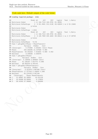
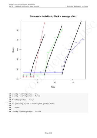
![No
com
m
ercialuse
Single-case data analysis: Resources
16.21 Two-level models for data analysis Manolov, Moeyaert, & Evans
CaseStandardnormalquantiles
−1.0
−0.5
0.0
0.5
1.0
−3 −2 −1 0 1 2 3
(Intercept)
−10 0 10 20
Phase
−5 0 5 10
−1.0
−0.5
0.0
0.5
1.0
PhaseTimecntr
## Linear mixed model fit by REML ['lmerMod']
## Formula: Score ~ 1 + Phase + PhaseTimecntr + (1 + Phase + PhaseTimecntr |
## Case)
## Data: Dataset2
## REML criterion at convergence: 162.7101
## Random effects:
## Groups Name Std.Dev. Corr
## Case (Intercept) 2.255
## Phase 14.192 -0.99
## PhaseTimecntr 7.634 -0.89 0.94
## Residual 3.009
## Number of obs: 31, groups: Case, 3
## Fixed Effects:
## (Intercept) Phase PhaseTimecntr
## 34.12 40.92 9.39
## (Intercept) Phase PhaseTimecntr
## 34.115142 40.921401 9.389626
## $Case
Page 383](https://image.slidesharecdn.com/635a0af9-e378-45de-b512-1e1e88e419b8-160210073243/85/Tutorial-387-320.jpg)

![No
com
m
ercialuse
Single-case data analysis: Resources
16.21 Two-level models for data analysis Manolov, Moeyaert, & Evans
In the following alternative models are presented for the same data.
# Alternative model # 1
# Specify the model
Multilevel.null <- lme(Score~1,
random=~1|Case,data=Dataset2,
control=list(opt="optim"))
# Copy and paste the rest of the code in the R console
fit <- fitted(Multilevel.null)
fit <- fitted(Multilevel.null)
Dataset2$fit <- fit
par(mfrow=c(2,2))
plot(Score[Case==1]~Time[Case==1], data=Dataset2, xlab="Time",
ylab="Score", xlim=c(1,max(Dataset2$Time)),
ylim=c(min(Dataset2$Score), max(Dataset2$Score)))
for (i in 1:tiers)
{
points(Score[Case==i]~Time[Case==i], col=cols[i],data=Dataset2)
lines(Dataset2$Time[Dataset2$Case==i],
Dataset2$fit[Dataset2$Case==i], col=cols[i])
}
title(main="Null model")
# Alternative model # 2
# Specify the model
Multilevel.phase.random <- lme(Score~1+Phase,
random=~1+Phase|Case,
data=Dataset2,
control=list(opt="optim"))
# Copy and paste the rest of the code in the R console
fit <- fitted(Multilevel.phase.random)
Dataset2$fit <- fit
plot(Score[Case==1]~Time[Case==1], data=Dataset2, xlab="Time",
ylab="Score", xlim=c(1,max(Dataset2$Time)),
ylim=c(min(Dataset2$Score), max(Dataset2$Score)))
for (i in 1:tiers)
{
points(Score[Case==i]~Time[Case==i], col=cols[i],data=Dataset2)
lines(Dataset2$Time[Dataset2$Case==i],
Dataset2$fit[Dataset2$Case==i], col=cols[i])
}
title(main="Random intercept & change in level")
Page 385](https://image.slidesharecdn.com/635a0af9-e378-45de-b512-1e1e88e419b8-160210073243/85/Tutorial-389-320.jpg)
![No
com
m
ercialuse
Single-case data analysis: Resources
16.21 Two-level models for data analysis Manolov, Moeyaert, & Evans
# Alternative model # 3
# Specify the model
Multilevel.time <- lme(Score~1+Time,random=~1|Case,
data=Dataset2,
control=list(opt="optim"),na.action="na.omit")
# Copy and paste the rest of the code in the R console
fit <- fitted(Multilevel.time)
Dataset2$fit <- fit
plot(Score[Case==1]~Time[Case==1], data=Dataset2, xlab="Time",
ylab="Score", xlim=c(1,max(Dataset2$Time)),
ylim=c(min(Dataset2$Score), max(Dataset2$Score)))
for (i in 1:tiers)
{
points(Score[Case==i]~Time[Case==i], col=cols[i],data=Dataset2)
lines(Dataset2$Time[Dataset2$Case==i],
Dataset2$fit[Dataset2$Case==i], col=cols[i])
}
title(main="Trend & random intercept")
# Alternative model # 4
# Specify the model
Multilevel.sc <- lme(Score~1+Time+PhaseTimecntr,
random=~Time+PhaseTimecntr|Case,data=Dataset2,
control=list(opt="optim"))
# Copy and paste the rest of the code in the R console
fit <- fitted(Multilevel.sc)
Dataset2$fit <- fit
plot(Score[Case==1]~Time[Case==1], data=Dataset2, xlab="Time",
ylab="Score", xlim=c(1,max(Dataset2$Time)),
ylim=c(min(Dataset2$Score), max(Dataset2$Score)))
for (i in 1:tiers)
{
points(Score[Case==i]~Time[Case==i], col=cols[i],
data=Dataset2)
lines(Dataset2$Time[Dataset2$Case==i],
Dataset2$fit[Dataset2$Case==i], col=cols[i])
}
title(main="Random trend & change in trend")
Page 386](https://image.slidesharecdn.com/635a0af9-e378-45de-b512-1e1e88e419b8-160210073243/85/Tutorial-390-320.jpg)
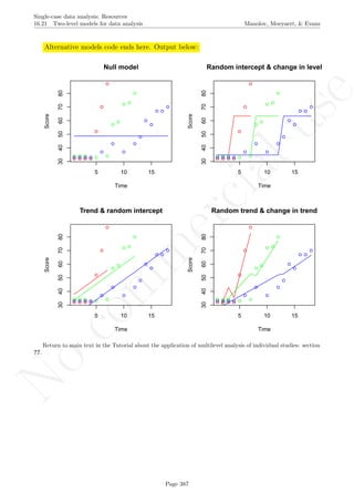
![No
com
m
ercialuse
Single-case data analysis: Resources
16.22 Meta-analysis using the SCED-specific standardized mean difference Manolov, Moeyaert, & Evans
16.22 Meta-analysis using the SCED-specific standardized mean difference
This code is applicable to any effect size index for which the inverse variance can be obtained (via knowledge
of the sampling distribution) and can be used as a weight.
This code requires that the metafor package for R (which it loads). In case it has not been previously installed,
this is achieved in the R console via the following code:
install.packages('metafor')
# Input data: copy-paste line and load
# /locate the data matrix
DataD <- read.table(file.choose(),header=TRUE)
Data matrix aspect as shown below:
## Id ES Variance
## Ninci_prompt 2.71 0.36
## Foxx_A 4.17 0.74
## Foxx_1973 4.42 1.02
# Copy and paste the rest of the code in the R console
# Load the previously installed "metafor" package
# needed for the forest plot
require(metafor)
# Number of studies / effect sizes being integrated
studies <- dim(DataD)[1]
# Effect sizes for the different studies
d_unsorted <- DataD$ES
# Study identifiers
etiq <- DataD$Id
# Weights for the different studies
vi_unsorted <- DataD$Variance
vi <- rep(0,length(d_unsorted))
etiqsort <- rep(0,length(d_unsorted))
# Sort the effect sizes
d <- sort(d_unsorted)
orders <- sort(d_unsorted,index.return=T)$ix
for (i in 1:studies)
{
etiqsort[i] <- as.character(etiq[orders[i]])
vi[i] <- vi_unsorted[orders[i]]
}
# Obtain the weighted average
rma(yi=d,vi=vi)
w.average <- rma(yi=d,vi=vi)[[1]]
lower <- rma(yi=d,vi=vi)$ci.lb
upper <- rma(yi=d,vi=vi)$ci.ub
Page 388](https://image.slidesharecdn.com/635a0af9-e378-45de-b512-1e1e88e419b8-160210073243/85/Tutorial-392-320.jpg)

![No
com
m
ercialuse
Single-case data analysis: Resources
16.22 Meta-analysis using the SCED-specific standardized mean difference Manolov, Moeyaert, & Evans
1.00 3.00 5.00 7.00
Observed Outcome
Foxx_1973
Foxx_A
Ninci_prompt
4.42 [ 2.44 , 6.40 ]
4.17 [ 2.48 , 5.86 ]
2.71 [ 1.53 , 3.89 ]
3.57 [ 2.41 , 4.74 ]
Effect sizes per study
Weighted average
Return to main text in the Tutorial about the meta-analysis using the HPS d-statistic: section 11.1.
Page 390](https://image.slidesharecdn.com/635a0af9-e378-45de-b512-1e1e88e419b8-160210073243/85/Tutorial-394-320.jpg)
![No
com
m
ercialuse
Single-case data analysis: Resources
16.23 Meta-analysis using the MPD and SLC Manolov, Moeyaert, & Evans
16.23 Meta-analysis using the MPD and SLC
This code is applicable to any effect size index for which the researcher desires to obtain a weighted average,
even if the weight is not the inverse variance of the effect size index. In case inverse variance is not known,
confidence intervals cannot be obtained and the intervals in the modified forest plot represent ranges of values.
This code requires that the metafor package for R (which it loads). In case it has not been previously
installed, this is achieved in the R console via the following code:
install.packages('metafor')
# Input data: copy-paste line and load
# /locate the data matrix
DataMPD <- read.table(file.choose(),header=TRUE,fill=TRUE)
Data matrix aspect as shown below:
## Id ES weight Tier1 Tier2 Tier3 Tier4 Tier5
## Jones 2.0 3.0 1 2 3 NA NA
## Phillips 3.0 3.6 2 2 5 6 NA
## Mario 6.0 4.0 4 6 6 6 NA
## Alma 7.0 2.0 3 5 7 NA NA
## P´erez 2.2 2.5 1 1 3 3 4
## Hibbs 1.5 1.0 -1 1 3 NA NA
## Petrov 3.1 1.7 2 4 6 6 3
# Copy and paste the rest of the code in the R console
# Number of studies being meta-analyzed
studies <- dim(DataMPD)[1]
# Effect sizes for the different studies
es <- DataMPD$ES
# Study identifiers
etiq <- DataMPD$Id
# Weights for the different studies
weight <- DataMPD$weight
w_sorted <- rep(0,length(weight))
# Maximum number of tiers in any of the studies
max.tiers <- dim(DataMPD)[2]-3
# Outcomes obtained for each of the baselines
# in each of the studies
studies.alleffects <- DataMPD[,(4:dim(DataMPD)[2])]
# Obtain the across-studies weighted average
stdES_num <- 0
for (i in 1:studies)
stdES_num <- stdES_num + es[i]*weight[i]
stdES_den <- sum(weight)
stdES <- stdES_num / stdES_den
# Creation of the FOREST PLOT
# Bounds for the confidence interval on the basis of ES-ranges per study
upper <- rep(0,studies)
Page 391](https://image.slidesharecdn.com/635a0af9-e378-45de-b512-1e1e88e419b8-160210073243/85/Tutorial-395-320.jpg)
![No
com
m
ercialuse
Single-case data analysis: Resources
16.23 Meta-analysis using the MPD and SLC Manolov, Moeyaert, & Evans
lower <- rep(0,studies)
for (i in 1:studies)
{
upper[i] <- suppressWarnings(max(as.numeric(
+ studies.alleffects[i,]),na.rm=TRUE))
lower[i] <- suppressWarnings(min(as.numeric(
+ studies.alleffects[i,]),na.rm=TRUE))
}
# Call the R package required for creating the forest plot
require(metafor)
# Sort the effect sizes and the labels for the studies
es_sorted <- sort(es)
# Sort the labels for the studies according
# to the sorted effect sizes
etiqsort <- rep(0,studies)
orders <- sort(es,index.return=T)$ix
for (i in 1:studies)
etiqsort[i] <- as.character(etiq[orders[i]])
# Sort the min-max boundaries of the ranges for the studies
# according to the sorted effect sizes
up_sort <- rep(0,studies)
low_sort <- rep(0,studies)
for (i in 1:studies)
{
up_sort[i] <- upper[orders[i]]
low_sort[i] <- lower[orders[i]]
w_sorted[i] <- weight[orders[i]]
}
# Size of box according to weight
ave_w <- round(mean(weight),digits=0)
# Obtain the forest plot (ES in ascending order)
forest(es_sorted,ci.lb=low_sort,ci.ub=up_sort,
psize=2*w_sorted/(2*ave_w), ylim=c(-2.5,(studies+3)),
slab=etiqsort)
# Add the weighted average
addpoly.default(stdES,ci.lb=min(es),ci.ub=max(es),
rows=-2,annotate=TRUE,efac=4,cex=1)
# Add lables
leftest <- min(lower)-max(upper)
rightest <- 2*max(upper)
text(leftest, -2, "Weighted average", pos=4, cex=1)
text(leftest, (studies+2), "Study Id", pos=4, cex=1)
text(rightest, (studies+2), "ES per study [Range]",
pos=2, cex=1)
abline(h=0)
Page 392](https://image.slidesharecdn.com/635a0af9-e378-45de-b512-1e1e88e419b8-160210073243/85/Tutorial-396-320.jpg)
![No
com
m
ercialuse
Single-case data analysis: Resources
16.23 Meta-analysis using the MPD and SLC Manolov, Moeyaert, & Evans
Code ends here. Default output of the code below:
−2.00 2.00 4.00 6.00 8.00
Observed Outcome
Alma
Mario
Petrov
Phillips
Pérez
Jones
Hibbs
7.00 [ 3.00 , 7.00 ]
6.00 [ 4.00 , 6.00 ]
3.10 [ 2.00 , 6.00 ]
3.00 [ 2.00 , 6.00 ]
2.20 [ 1.00 , 4.00 ]
2.00 [ 1.00 , 3.00 ]
1.50 [ −1.00 , 3.00 ]
3.77 [ 1.50 , 7.00 ]Weighted average
Study Id ES per study [Range]
Return to main text in the Tutorial about the meta-analysis using the Mean phase difference or the Slope
and level change: section 11.2.
Page 393](https://image.slidesharecdn.com/635a0af9-e378-45de-b512-1e1e88e419b8-160210073243/85/Tutorial-397-320.jpg)

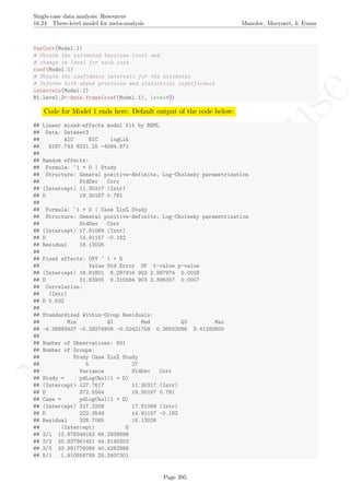
![No
com
m
ercialuse
Single-case data analysis: Resources
16.24 Three-level model for meta-analysis Manolov, Moeyaert, & Evans
## 5/2 1.119135444 36.9854822
## 5/3 49.968498046 56.1822312
## 5/4 -0.838468123 3.1664840
## 5/5 -0.422106076 2.3922718
## 5/6 41.415148845 6.7482128
## 9/1 0.009326098 2.1927599
## 9/2 0.532902610 2.3238938
## 9/3 -0.109239850 0.5483110
## 9/4 -0.046104222 0.6811297
## 9/5 3.361893514 12.1847058
## 9/6 -0.085993488 0.5544554
## 15/1 28.880708304 31.6478697
## 15/2 34.953017292 42.3777182
## 15/3 4.818400887 43.8848292
## 15/4 4.088130431 43.1857527
## 15/5 21.078235875 38.3582981
## 15/6 39.407670550 41.7792769
## 15/7 53.872118564 29.9046202
## 15/8 61.208614052 14.4302311
## 15/9 51.841159767 26.2042253
## 16/1 10.193555494 63.0545996
## 16/2 14.623522745 48.1476058
## 16/3 16.935427965 50.3902948
## Approximate 95% confidence intervals
##
## Fixed effects:
## lower est. upper
## (Intercept) 6.457755 18.81801 31.17827
## D 13.356333 31.63905 49.92176
## attr(,"label")
## [1] "Fixed effects:"
##
## Random Effects:
## Level: Study
## lower est. upper
## sd((Intercept)) 4.2188182 11.303171 30.2837586
## sd(D) 8.3528764 19.301667 44.6019247
## cor((Intercept),D) -0.8780818 0.781117 0.9980412
## Level: Case
## lower est. upper
## sd((Intercept)) 12.927363 17.8106934 24.5387089
## sd(D) 10.397661 14.9115698 21.3850889
## cor((Intercept),D) -0.579575 -0.1820918 0.2853823
##
## Within-group standard error:
## lower est. upper
## 17.30152 18.13026 18.99870
Page 396](https://image.slidesharecdn.com/635a0af9-e378-45de-b512-1e1e88e419b8-160210073243/85/Tutorial-400-320.jpg)


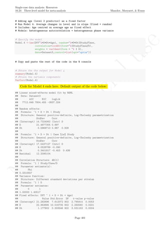


This document provides a tutorial on using software resources, mainly the R programming language, to analyze single-case experimental design data. It covers topics such as visual analysis techniques, calculation of nonoverlap indices, regression analyses, randomization tests, simulation modeling, and methods for integrating results across multiple studies. Step-by-step guidance is provided for using R and related packages to conduct these various quantitative analyses and visualize results. Relevant code is included in appendices. Aimed at applied researchers, the tutorial is a guide to computational methods for analyzing single-subject data.