The document provides an overview of statistics and its significance in data analytics, touching upon the fundamentals of statistical analysis, different types of data, and their applications in various fields. It discusses categorical and numerical data, including their characteristics, measurement levels, and appropriate statistical methods for analysis. Additionally, it includes practical examples and Python code snippets for data analysis techniques such as correlation, linear regression, and hypothesis testing.

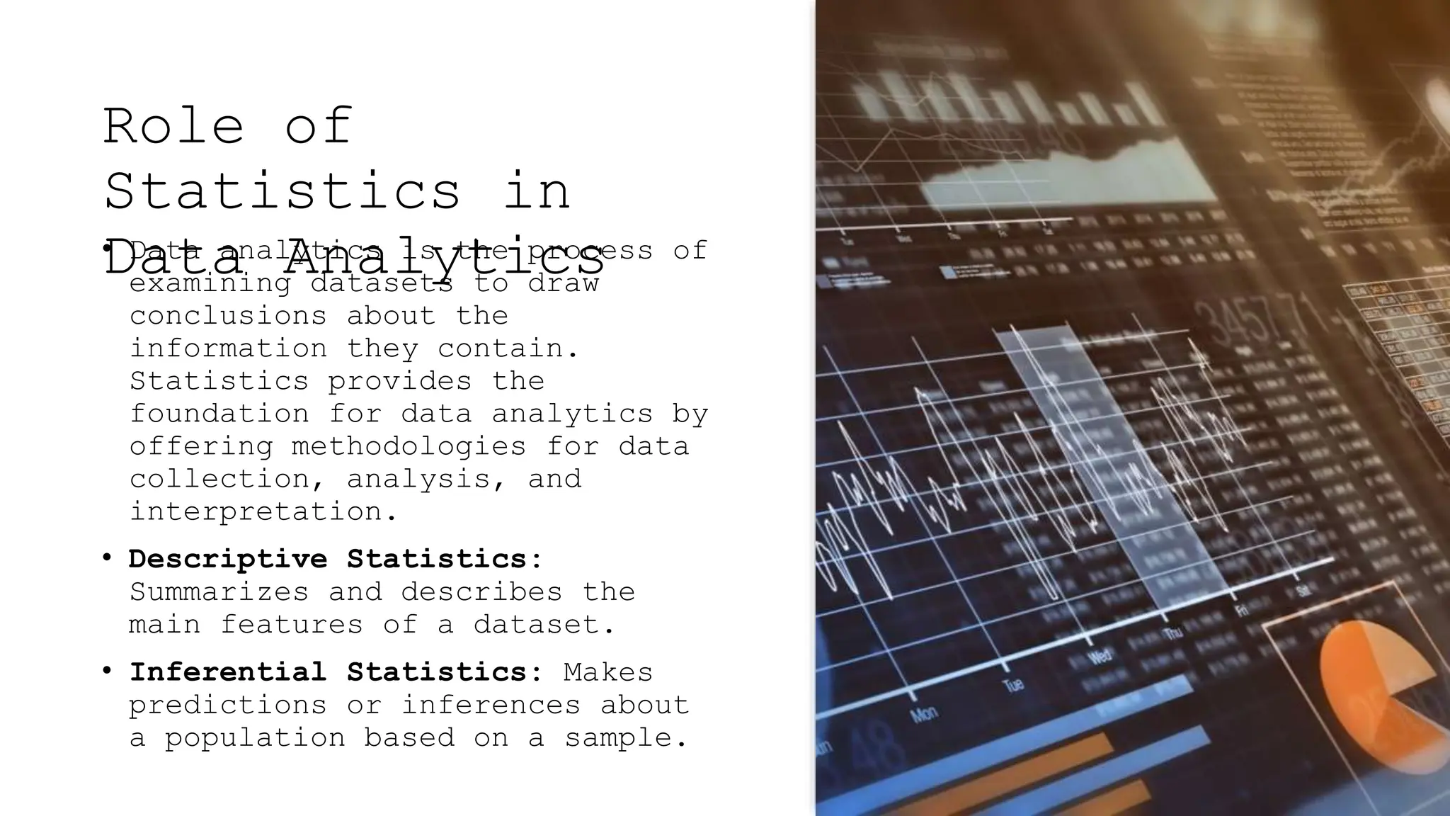
1. Statistics for Data
Analysis
Jeffhraim Balilla MBA,MoS

2. Lecture 1: Overview
of Statistics and
its Relevance in
Data Analytics
Today’s Plans:
• Understand the role of
statistics in data
analytics and the basics of
statistical analysis.
• Definition and importance
of statistics
• Applications of statistics
in various fields
• How statistics aids in
decision-making and
problem-solving

3. What is
Statistics?
• Statistics is a branch of
mathematics dealing with data
collection, analysis,
interpretation, and
presentation.
• Statistics involves the study
of methods for collecting,
analyzing, interpreting, and
presenting empirical data. It
provides tools for
understanding patterns,
trends, and relationships
within data. By transforming
raw data into meaningful
information, statistics helps
us to make evidence-based
decisions.

4. Applications of
Statistics
• Business: Market research,
quality control, financial
analysis.
• Healthcare: Epidemiology,
clinical trials, public health
studies.Government:
• Policy making, census data
analysis, economic planning.
• Academia and Research:
Hypothesis testing, experiment
design, survey analysis.

5. Role of
Statistics in
Data Analytics
• Data analytics is the process of
examining datasets to draw
conclusions about the
information they contain.
Statistics provides the
foundation for data analytics by
offering methodologies for data
collection, analysis, and
interpretation.
• Descriptive Statistics:
Summarizes and describes the
main features of a dataset.
• Inferential Statistics: Makes
predictions or inferences about
a population based on a sample.

6. Lecture 2: Types
of Data:
Categorical and
Numerical
• Data can be categorized into
different types, each with
unique characteristics and
applications. Understanding the
types of data is fundamental
for selecting appropriate
statistical methods and
analysis techniques.

7. Categorical Data
Categorical data, also known as
qualitative data, represents
characteristics or attributes that
can be grouped into categories.
Nominal Data: Categories with no
inherent order (e.g., gender,
ethnicity, colors).
Ordinal Data: Categories with a
meaningful order but no fixed
interval between them (e.g.,
rankings, education levels).

8. Some examples
• Frequency Counts and Mode (typical starting stats for
categ)
import pandas as pd
# Sample nominal data
data = {'Color': ['Red', 'Blue', 'Green',
'Blue', 'Red', 'Green', 'Red']}
df = pd.DataFrame(data)
# Frequency counts
frequency_counts = df['Color'].value_counts()
print(frequency_counts)
# Mode
mode = df['Color'].mode()
print(f'Mode: {mode[0]}')

9. Chi-Square
Test
The chi-square test is used to determine if there is a significant association between two nominal variables.
import pandas as pd
from scipy.stats import chi2_contingency
# Sample nominal data
data = {'Gender': ['Male', 'Female', 'Female', 'Male', 'Female', 'Male', 'Male'],
'Preference': ['Yes', 'No', 'Yes', 'Yes', 'No', 'No', 'Yes']}
df = pd.DataFrame(data)
# Contingency table
contingency_table = pd.crosstab(df['Gender'], df['Preference'])
print(contingency_table)
# Chi-square test
chi2, p, dof, ex = chi2_contingency(contingency_table)
print(f'Chi-square: {chi2}, p-value: {p}')

10. Median
and
Interqua
rtile
Range
(IQR)
import pandas as pd
# Sample ordinal data
data = {'Satisfaction': [3, 1,
4, 2, 5, 3, 4, 2, 1, 5]}
df = pd.DataFrame(data)
# Median
median =
df['Satisfaction'].median()
print(f'Median: {median}')
# Interquartile Range (IQR)
iqr =
df['Satisfaction'].quantile(0.
75) -
df['Satisfaction'].quantile(0.
25)
print(f'IQR: {iqr}')

11. Numerical Data
• Numerical data, also known as
quantitative data, represents
measurable quantities.
• Interval Data: Numeric data with
meaningful intervals between
values, but no true zero point
(e.g., temperature in Celsius).
• Ratio Data: Numeric data with
meaningful intervals and a true
zero point (e.g., height,
weight, age).

12. Key
Differences
• Measurement Level:
Categorical data is
measured using categories,
while numerical data is
measured using numbers.
• Statistical Analysis:
Categorical data is often
analyzed using frequency
counts and proportions,
while numerical data is
analyzed using measures of
central tendency and
variability.

13. Some examples
• Mean and Standard Deviation
import numpy as np
# Sample interval data (e.g.,
temperatures in Celsius)
temperatures = [23, 25, 22, 20, 26,
21, 24, 27, 23, 22]
# Mean
mean_temp = np.mean(temperatures)
print(f'Mean Temperature:
{mean_temp}')
# Standard Deviation
std_dev_temp = np.std(temperatures)
print(f'Standard Deviation of
Temperature: {std_dev_temp}')

14. Correlation and
Linear
Regression
• import numpy as np
• import matplotlib.pyplot
as plt
• from scipy.stats import
linregress
• # Sample interval data
(e.g., temperatures and
ice cream sales)
• temperatures = [23, 25,
22, 20, 26, 21, 24, 27,
23, 22]
• ice_cream_sales = [150,
160, 140, 130, 170, 135,
155, 180, 150, 140]
• # Correlation
• correlation =
np.corrcoef(temperatures,
ice_cream_sales)[0, 1]
• print(f'Correlation:
{correlation}')

15. Correlation and
Linear
Regression
• # Linear Regression
• slope, intercept, r_value,
p_value, std_err =
linregress(temperatures,
ice_cream_sales)
• print(f'Slope: {slope},
Intercept: {intercept}, R-
squared: {r_value**2}')
• # Plotting
• plt.scatter(temperatures,
ice_cream_sales, label='Data
points')
• plt.plot(temperatures,
np.array(temperatures)*slope +
intercept, color='red',
label='Regression line')
• plt.xlabel('Temperature
(Celsius)')
• plt.ylabel('Ice Cream Sales')
• plt.legend()
• plt.show()

16. Independent T-
Test (Typical
A/B Testing)
• import numpy as np
• from scipy.stats import ttest_ind
• # Sample ratio data (e.g., weights in kg
for two groups)
• group_a_weights = [70, 75, 80, 85, 90,
95, 100]
• group_b_weights = [60, 65, 70, 75, 80,
85, 90]
• # Independent T-Test
• t_stat, p_value =
ttest_ind(group_a_weights,
group_b_weights)
• print(f'T-statistic: {t_stat}, p-value:
{p_value}')

17. Geometric Mean
and Coefficient
of Variation
• import numpy as np
• from scipy.stats import gmean
• # Sample ratio data (e.g., heights in
centimeters)
• heights = [150, 160, 170, 180, 190, 200,
210]
• # Geometric Mean
• geom_mean_height = gmean(heights)
• print(f'Geometric Mean of Heights:
{geom_mean_height}')
• # Coefficient of Variation
• mean_height = np.mean(heights)
• std_dev_height = np.std(heights)
• coef_var_height = (std_dev_height /
mean_height) * 100
• print(f'Coefficient of Variation:
{coef_var_height}%')

18. Practice
(Identification)
• Identify the levels of
measurement for the provided
variables:
• Type of Pet
• Temperature in Fahrenheit
• Rank in a Competition (1st, 2nd,
3rd)
• Height of Students in Centimeters
• Customer Satisfaction Rating
(Very Unsatisfied, Unsatisfied,
Neutral, Satisfied, Very
Satisfied)
• IQ Score
• Age in Years
• Number of Siblings

19. Data
Analysis
Tree

20. End