Chapter 1_Lect_3 System Modeling_144875f87dacff21abd64f918872013c Copy.pdf
1.
ECO 381
Control Engineering
Spring2024/2025
Egyptian Academy for Engineering and
Advanced Technology
Cadets: 3rd Electrical
1
Electrical Engineering Department
Assoc. Prof./ Sameh Ghanem
samehghanem@eaeat-academy.edu.eg
2.
2
Course Outlines
Lecture No.Course description Notes
1 Introduction to control systems
2 Transfer function and block reduction systems
3 Mathematical model of electrical and mechanical systems Quiz 1
4 Transient response of control systems Assignment 1
5 Steady state response of control systems
6 Stability analysis by Routh’s criteria.
7 Control system analysis and design using Root Locus
8 Control system analysis and design using Root Locus Quiz 2
9 Compensation of control system (lead and lag compensator)
10 Control system analysis and design using frequency response (Bode plot) Assignment 2
11 Control system analysis and design using frequency response (Bode plot) Quiz 3
12 PID controller design
13 Revision Quiz 4
14 Final exam
Objectives
• Understand whymodeling is essential.
• Basic modeling process.
• Principle elements of Mechanical systems.
• Principle elements of Electrical systems.
• Transfer function.
5.
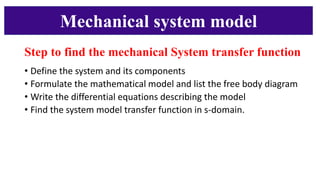
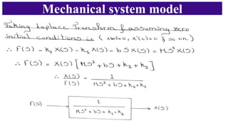
Mechanical system model
Stepto find the mechanical System transfer function
• Define the system and its components
• Formulate the mathematical model and list the free body diagram
• Write the differential equations describing the model
• Find the system model transfer function in s-domain.
1
2
3
4
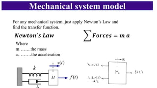
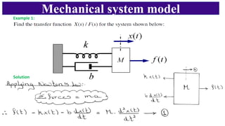
For any mechanicalsystem, just apply Newton’s Law and
find the transfer function.
𝑵𝒆𝒘𝒕𝒐𝒏′
𝒔 𝑳𝒂𝒘 𝑭𝒐𝒓𝒄𝒆𝒔 = 𝒎 𝒂
Where
m……..the mass
a………the acceleration
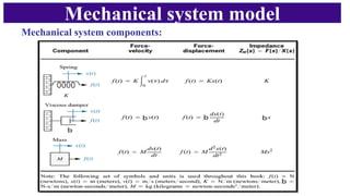
Mechanical system model
Mechanical system model
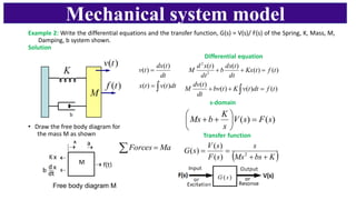
Example2: Write the differential equations and the transfer function, G(s) = V(s)/ F(s) of the Spring, K, Mass, M,
Damping, b system shown.
Solution
• Draw the free body diagram for
the mass M as shown
s-domain
)
(
)
( s
F
s
V
s
K
b
Ms =
+
+
)
(
)
(
)
(
)
(
2
2
t
f
t
Kx
dt
t
dx
b
dt
t
x
d
M =
+
+
Differential equation
Transfer function
( )
K
bs
Ms
s
s
F
s
V
s
G
+
+
=
= 2
)
(
)
(
)
(
Free body diagram M
= Ma
Forces
)
(
)
(
)
(
)
(
t
f
dt
t
v
K
t
bv
dt
t
dv
M =
+
+
=
=
dt
t
v
t
x
dt
t
dx
t
v
)
(
)
(
)
(
)
(
Mechanical system model
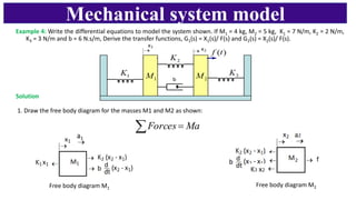
Example4: Write the differential equations to model the system shown. If M1 = 4 kg, M2 = 5 kg, K1 = 7 N/m, K2 = 2 N/m,
K3 = 3 N/m and b = 6 N.s/m, Derive the transfer functions, G1(s) = X1(s)/ F(s) and G2(s) = X2(s)/ F(s).
Solution
1. Draw the free body diagram for the masses M1 and M2 as shown:
Free body diagram M1
Free body diagram M2
= Ma
Forces
14.
Mechanical system model
Solution:
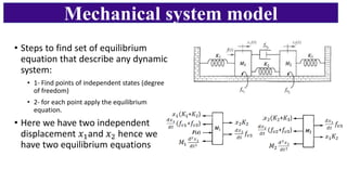
2.Write an equilibrium equation for each mass:
For the Mass M1
K2 [x2(t) – x1(t)] + b d/dt [x2(t) – x1(t)] – K1x1(t) - M1 d2/dt2 x1(t) = 0
Substitute the constant values, we get:
2 [x2(t) – x1(t)] + 6 d/dt [x2(t) – x1(t)] - 7 x1(t) – 4 d2/dt2 x1(t) = 0 (1)
For the Mass M2
f(t) - K3x2(t) - K2 [x2(t) – x1(t)] - b d/dt [x2(t) – x1(t)] – M2 d2/dt2 x2(t) = 0
5 d2/dt2 x2(t) + 2 [x2(t) – x1(t)] + 6 d/dt [x2(t) – x1(t)] + 3 x2(t) = f(t) (2)
• Collecting terms, the two simultaneous differential equations in x1(t) and x2(t), we
have:
4 d2/dt2 [x1(t)] + 6 d/dt [x1(t)] + 9 x1(t) - 6 d/dt [x2(t)] - 2 x2(t) = 0 (3)
- 6 d/dt [x1(t)] - 2 x1(t) + 5 d2/dt2 [x1(t) ]+ 6 d/dt [x2(t)] + 5 x2(t) = f(t) (4)
• Find the Laplace transform (3) and (4), we get:
(4s2 + 6s + 9) X1(s) – (6s + 2) X2(s) = 0 (5)
- (6s + 2) X1(s) + (5s2 + 6s + 5) X2(s) = F(s) (6)
• Eliminate X2(s) using (5) and (6) to get the transfer function G1(s) = X1(s)/ F(s).
• Eliminate X1(s) using (5) and (6) to get the transfer function G2(s) = X2(s)/ F(s).
15.
• Steps tofind set of equilibrium
equation that describe any dynamic
system:
• 1- Find points of independent states (degree
of freedom)
• 2- for each point apply the equilibrium
equation.
• Here we have two independent
displacement 𝑥1and 𝑥2 hence we
have two equilibrium equations
Mechanical system model
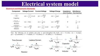
Resistor Inductor
Capacitor
Time DomainLaplace Domain
Component Voltage-Current Current-Voltage Voltage-Charge Impedance Admittance
Z(s)=V(s)/I(s) Y(s)=I(s)/V(s)
Electrical system model
Electrical and Electronic Elements
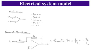
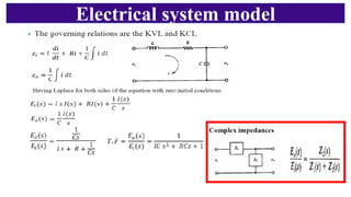
Electrical system model
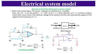
OperationalAmplifiers (Op Amps) in system control
• Refer to the shown figure, The closed – loop gain G is defined as G = C(s)/R(s)
Since r(t) = (V+ – V -) A, this yields V+ – V - = c/A = 0, (A ∞, I = 0) for ideal OP, so V+ = V– and this is called a
virtual short circuit means that whatever voltage at the positive terminal will automatically appears at the
negative terminal because A ∞.
( )
1
2
)
(
)
(
R
R
s
R
s
C
s
G −
=
=
Block diagram
( ) ( )
t
r
R
R
t
c
1
2
−
=
( )
( ) 1
2
)
(
Z
Z
s
R
s
C
s
G −
=
=
Inverting amplifier .
20.
Electrical system model
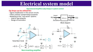
OperationalAmplifiers (Op Amps) in system control
Op Amps can be utilized for:
- Signal amplification in the sensor circuits
- Filters used for compensation purposes
- Modeling of the “real world” systems
- Lead or lag networks
- Design of controllers
Block diagram
( ) ( )
t
r
R
R
t
c
+
=
1
2
1 ( )
+
=
=
1
2
1
)
(
)
(
R
R
s
R
s
C
s
G
Non-inverting amplifier.
21.
Electrical system model
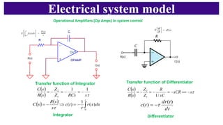
OperationalAmplifiers (Op Amps) in system control
Integrator
( )
( )
s
RCs
Z
Z
s
R
s
C 1
1
1
2
−
=
−
=
−
=
Transfer function of Integrator
( )
( )
s
sCR
sC
R
Z
Z
s
R
s
C
−
==
−
=
−
=
−
=
/
1
1
2
Transfer function of Differentiator
( ) ( )
−
=
−
=
t
dx
x
r
t
c
s
s
R
s
C
0
)
(
1
)
(
dt
t
dr
t
c
)
(
)
(
−
=
Integrator Differentiator
22.
Electrical system model
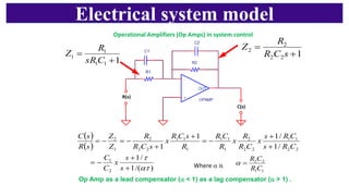
OperationalAmplifiers (Op Amps) in system control
1
1
1
1
1
+
=
C
sR
R
Z 1
2
2
2
2
+
=
s
C
R
R
Z
( )
( )
)
/(
1
/
1
/
1
/
1
1
1
2
1
2
2
1
1
2
2
2
1
1
1
1
1
1
2
2
2
1
2
+
+
−
=
+
+
−
=
+
+
−
=
−
=
s
s
x
C
C
C
R
s
C
R
s
x
C
R
R
x
R
C
R
R
s
C
R
x
s
C
R
R
Z
Z
s
R
s
C
1
1
2
2
C
R
C
R
=
Op Amp as a lead compensator ( < 1) as a lag compensator ( > 1) .
Where is
inverting ampifier
23.
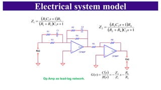
Electrical system model
()
( ) 1
1
1
3
1
3
1
1
1
+
+
+
=
s
C
R
R
R
s
C
R
Z
( )
( ) 1
1
2
4
2
4
2
2
2
+
+
+
=
s
C
R
R
R
s
C
R
Z
( )
( ) 5
6
1
2
)
(
R
R
x
Z
Z
s
R
s
C
s
G −
−
=
=
Op Amp as lead-lag network.
inverting amplifier
24.
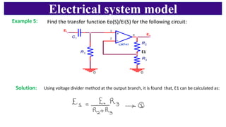
Electrical system model
Example5:
Solution:
Find the transfer function Eo(S)/Ei(S) for the following circuit:
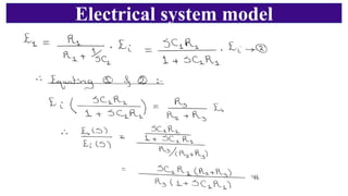
Using voltage divider method at the output branch, it is found that, E1 can be calculated as:
E1
Non-inverting amplifier
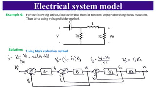
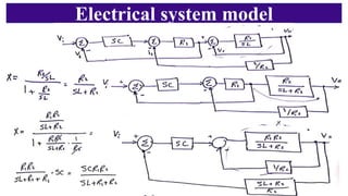
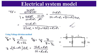
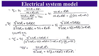
Electrical system model
+
-
ViVo
+
-
C L
R1 R2
For the following circuit, find the overall transfer function Vo(S)/Vi(S) using block reduction.
Then drive using voltage divider method.
Using block reduction method
Example 6:
Solution:
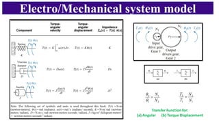
Transfer Function for:
(a)Angular (b) Torque Displacement
2
1
1
2
N
N
=
1
2
1
2
N
N
T
T
=
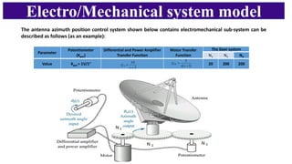
Electro/Mechanical system model
31.
Electro/Mechanical system model
Parameter
Potentiometer
(Kpot)
Differentialand Power Amplifier
Transfer Function
Motor Transfer
Function
The Geer system
N1 N2 N3
Value Kpot = 1V/1° 20 200 200
The antenna azimuth position control system shown below contains electromechanical sub-system can be
described as follows (as an example):
2
10
+
=
s
GA )
1
(
5
+
=
s
s
GM

![Mechanical system model
Solution:
2. Write an equilibrium equation for each mass:
For the Mass M1
K2 [x2(t) – x1(t)] + b d/dt [x2(t) – x1(t)] – K1x1(t) - M1 d2/dt2 x1(t) = 0
Substitute the constant values, we get:
2 [x2(t) – x1(t)] + 6 d/dt [x2(t) – x1(t)] - 7 x1(t) – 4 d2/dt2 x1(t) = 0 (1)
For the Mass M2
f(t) - K3x2(t) - K2 [x2(t) – x1(t)] - b d/dt [x2(t) – x1(t)] – M2 d2/dt2 x2(t) = 0
5 d2/dt2 x2(t) + 2 [x2(t) – x1(t)] + 6 d/dt [x2(t) – x1(t)] + 3 x2(t) = f(t) (2)
• Collecting terms, the two simultaneous differential equations in x1(t) and x2(t), we
have:
4 d2/dt2 [x1(t)] + 6 d/dt [x1(t)] + 9 x1(t) - 6 d/dt [x2(t)] - 2 x2(t) = 0 (3)
- 6 d/dt [x1(t)] - 2 x1(t) + 5 d2/dt2 [x1(t) ]+ 6 d/dt [x2(t)] + 5 x2(t) = f(t) (4)
• Find the Laplace transform (3) and (4), we get:
(4s2 + 6s + 9) X1(s) – (6s + 2) X2(s) = 0 (5)
- (6s + 2) X1(s) + (5s2 + 6s + 5) X2(s) = F(s) (6)
• Eliminate X2(s) using (5) and (6) to get the transfer function G1(s) = X1(s)/ F(s).
• Eliminate X1(s) using (5) and (6) to get the transfer function G2(s) = X2(s)/ F(s).](https://image.slidesharecdn.com/chapter1lect3systemmodeling144875f87dacff21abd64f918872013ccopy-250417094517-7376144f/85/Chapter-1_Lect_3-System-Modeling_144875f87dacff21abd64f918872013c-Copy-pdf-14-320.jpg)