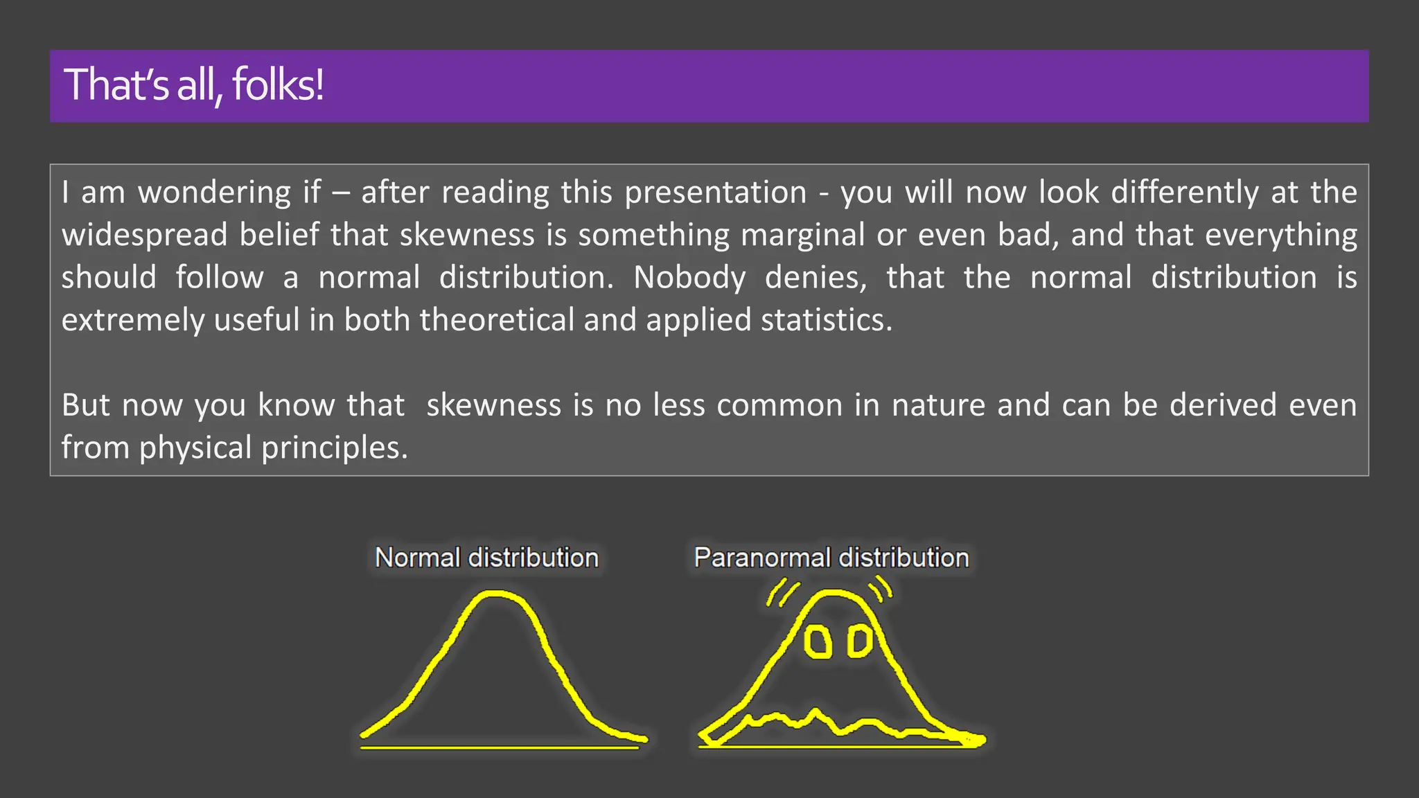
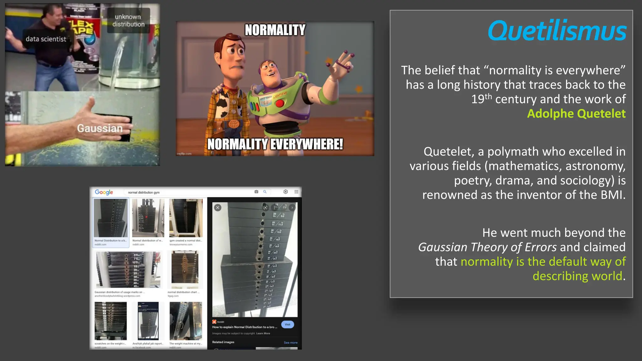
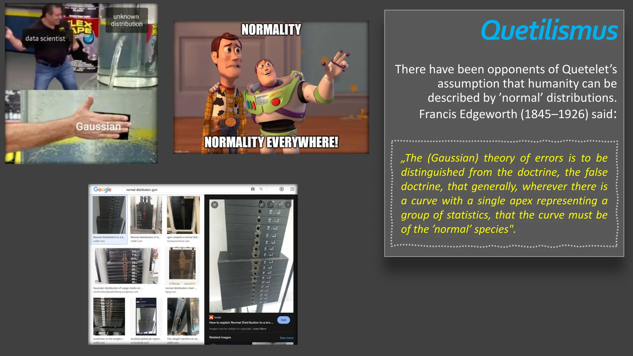
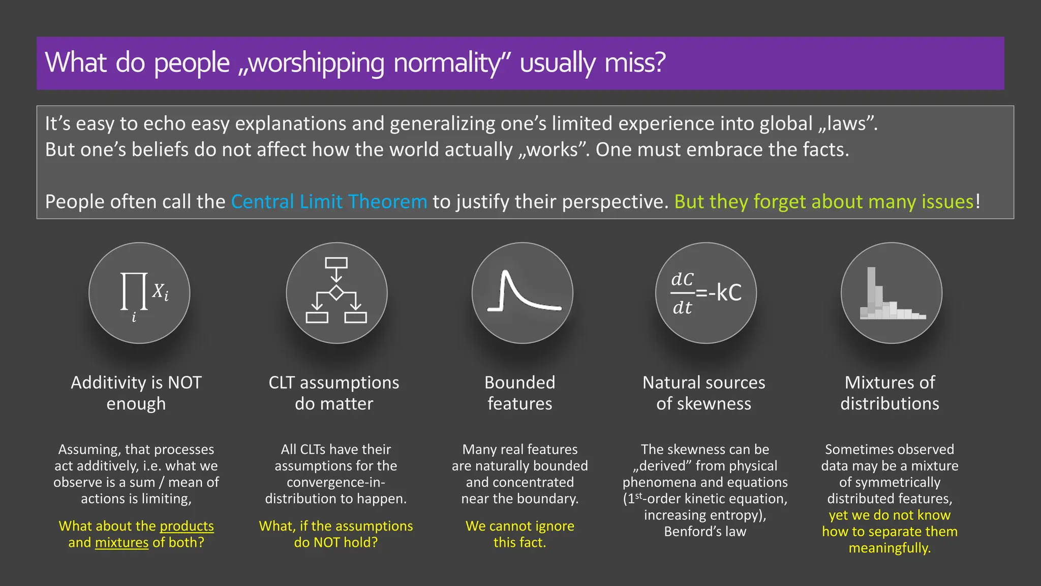
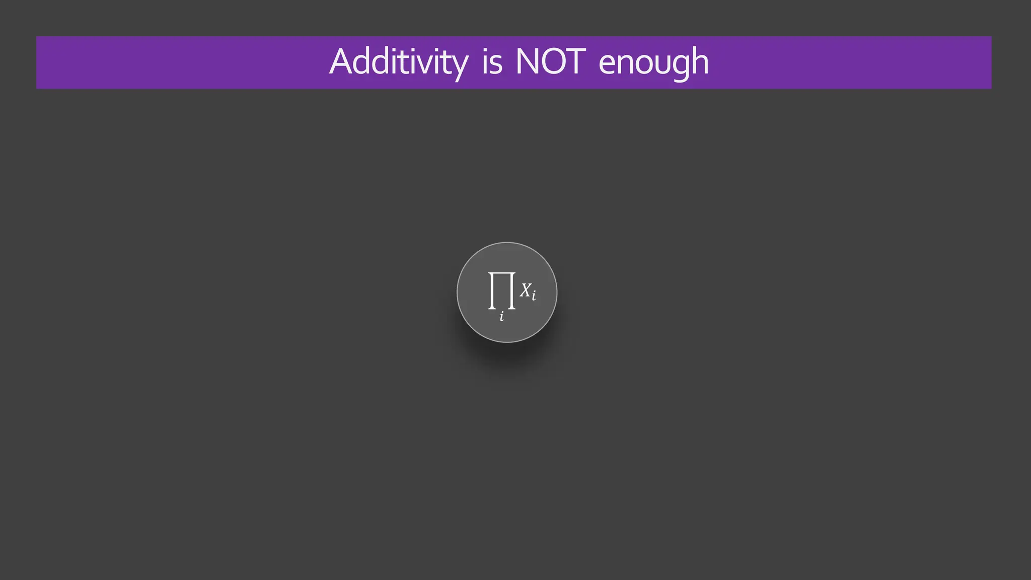
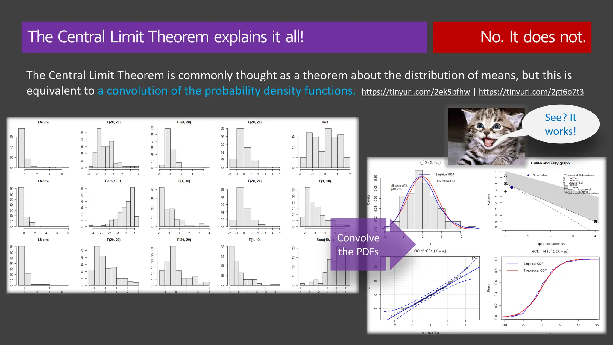
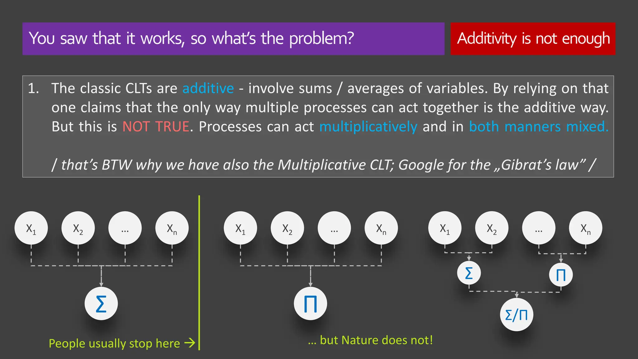
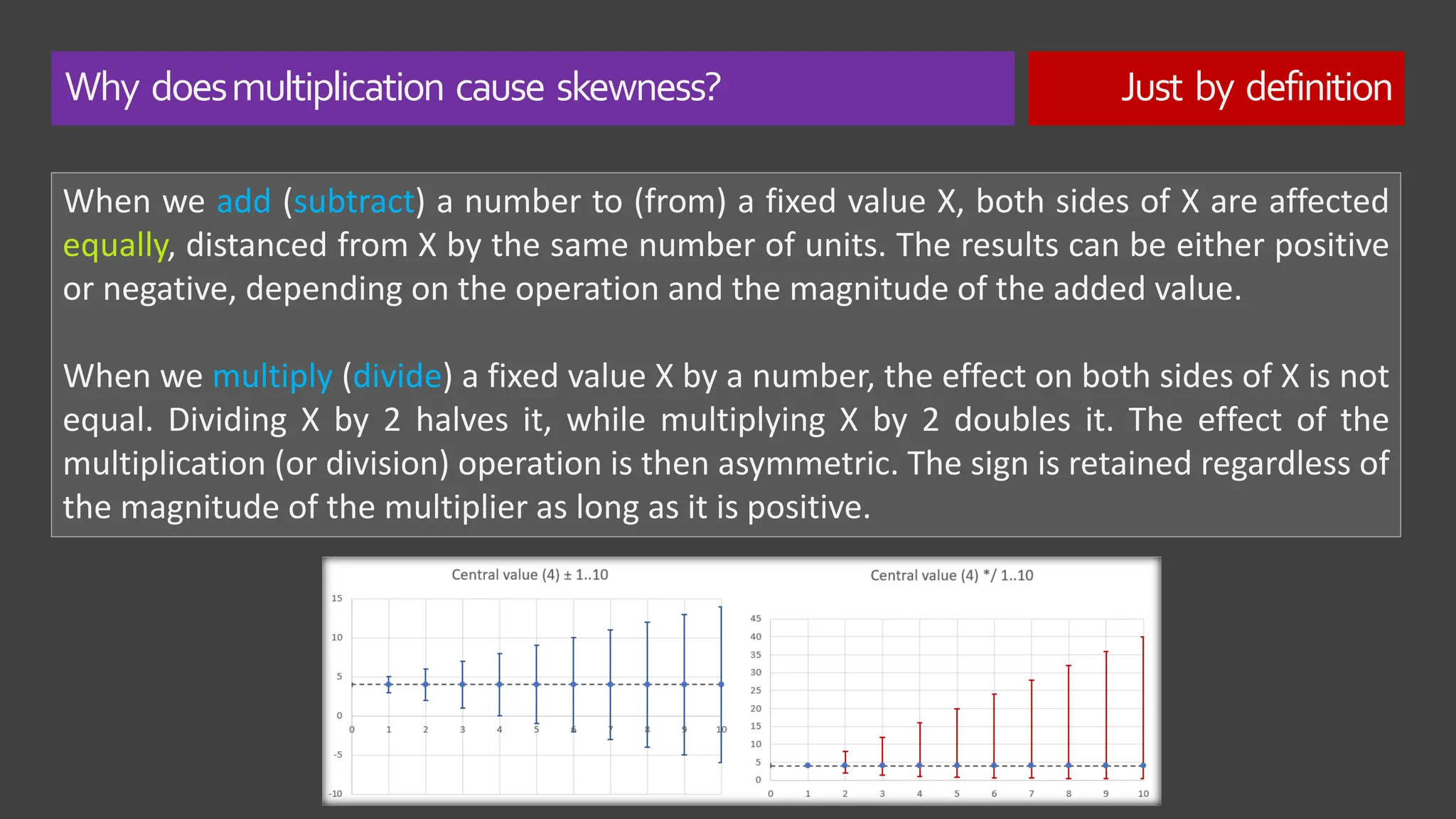
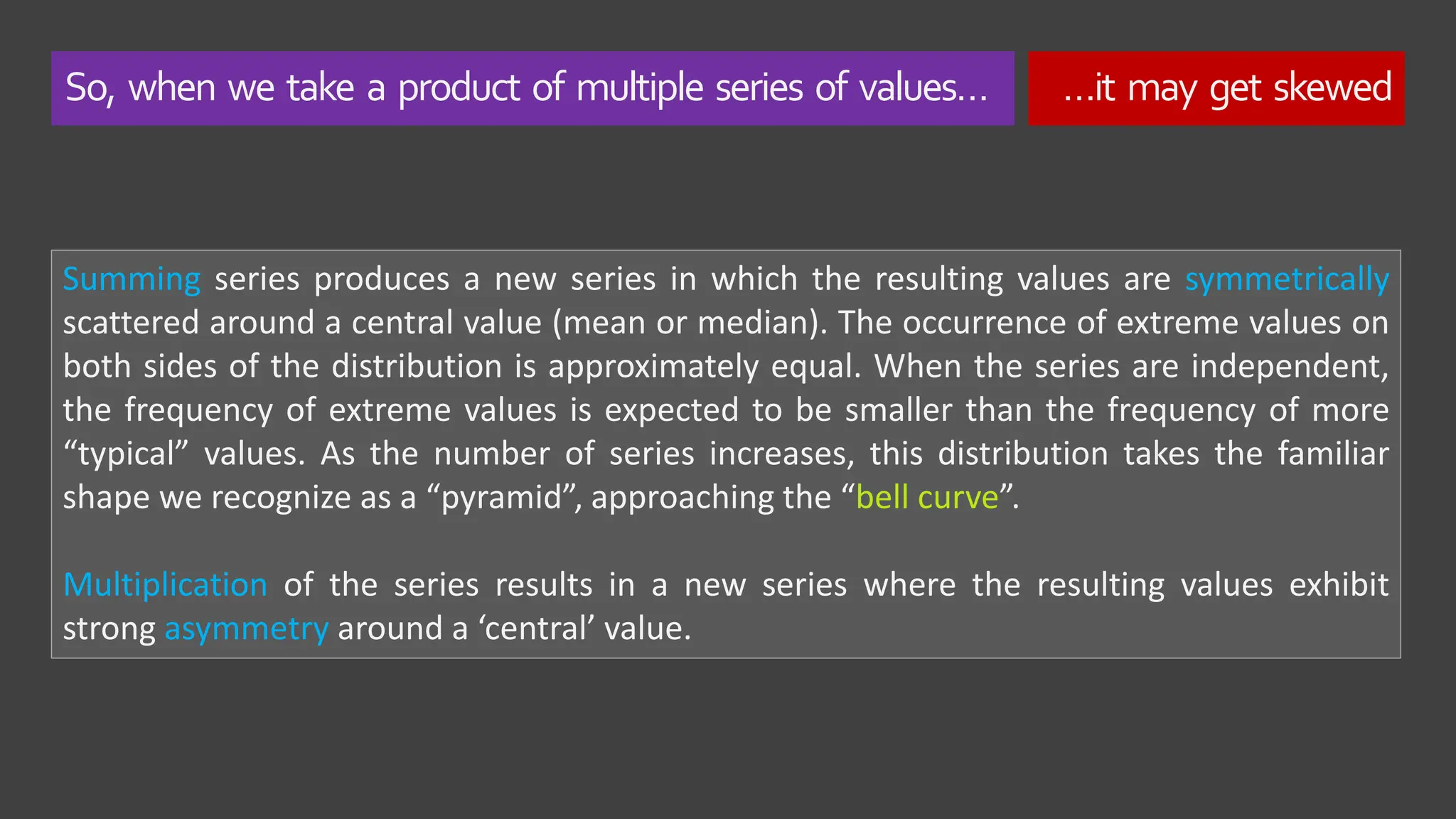
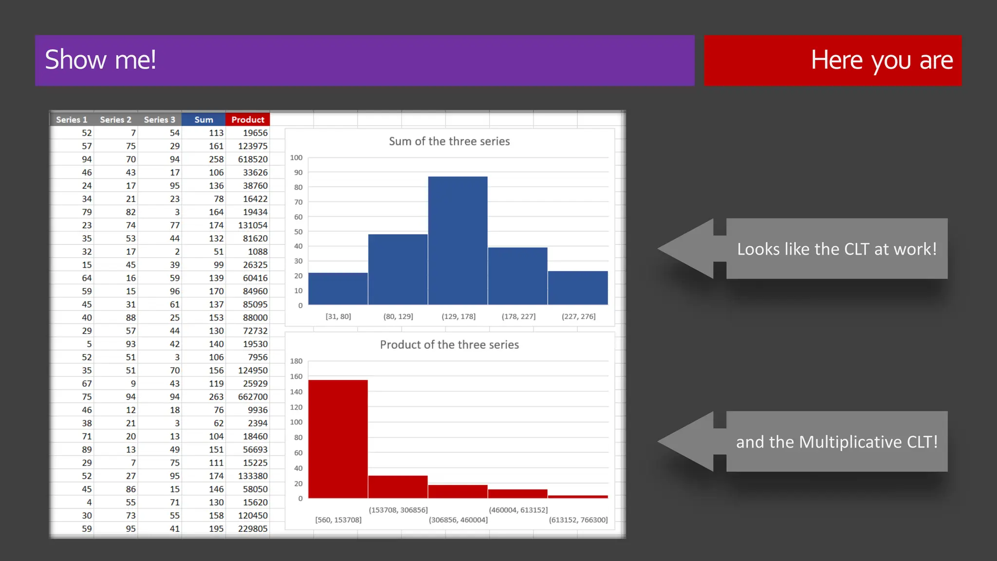
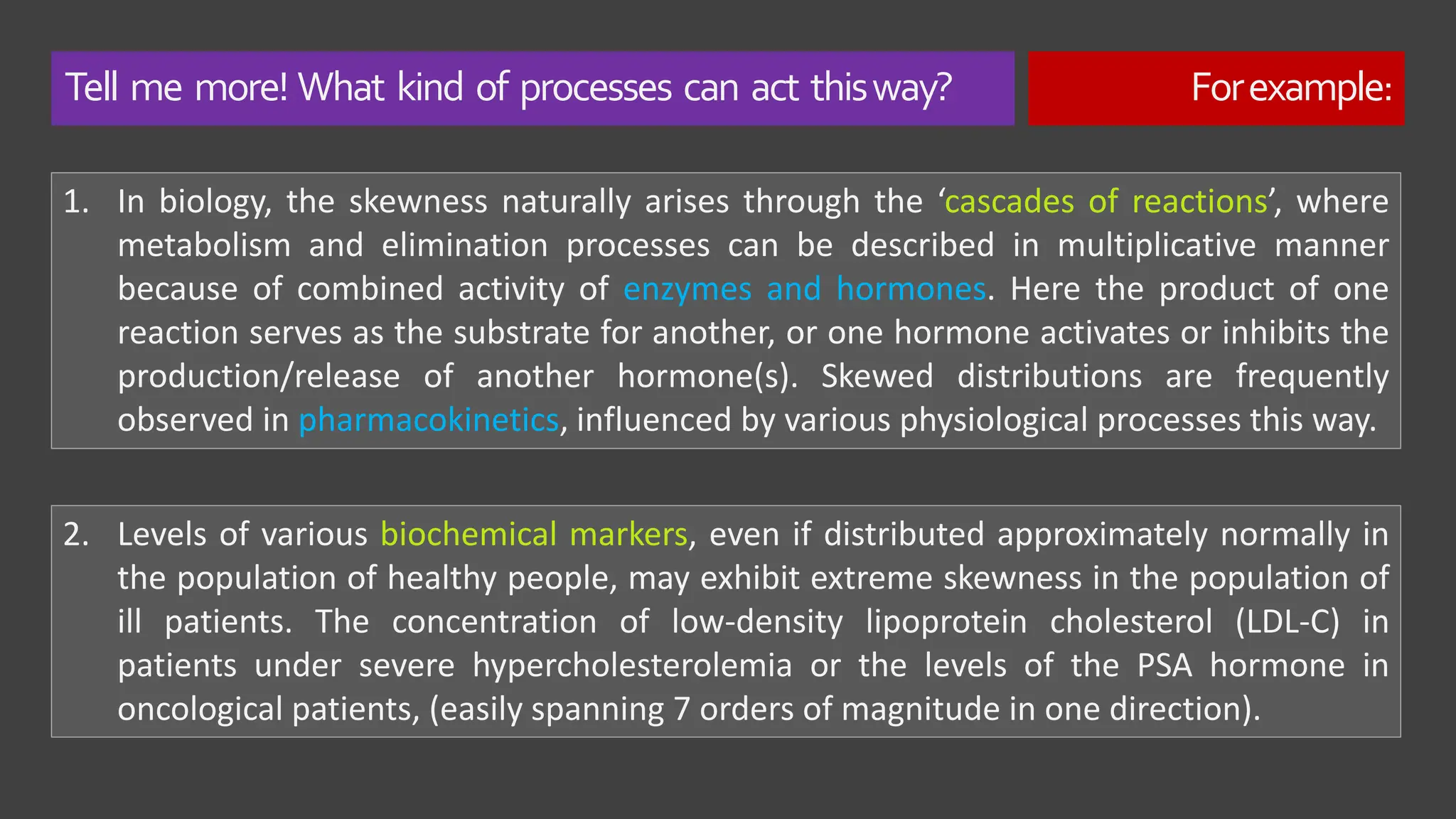
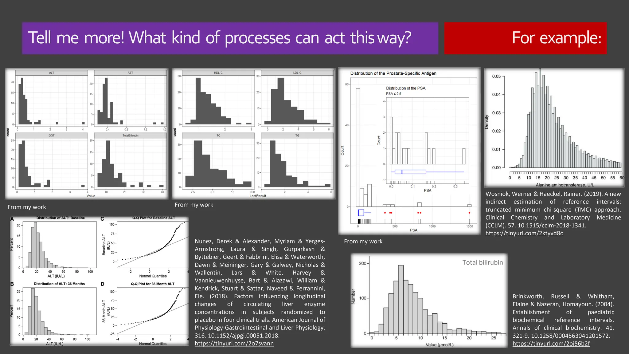
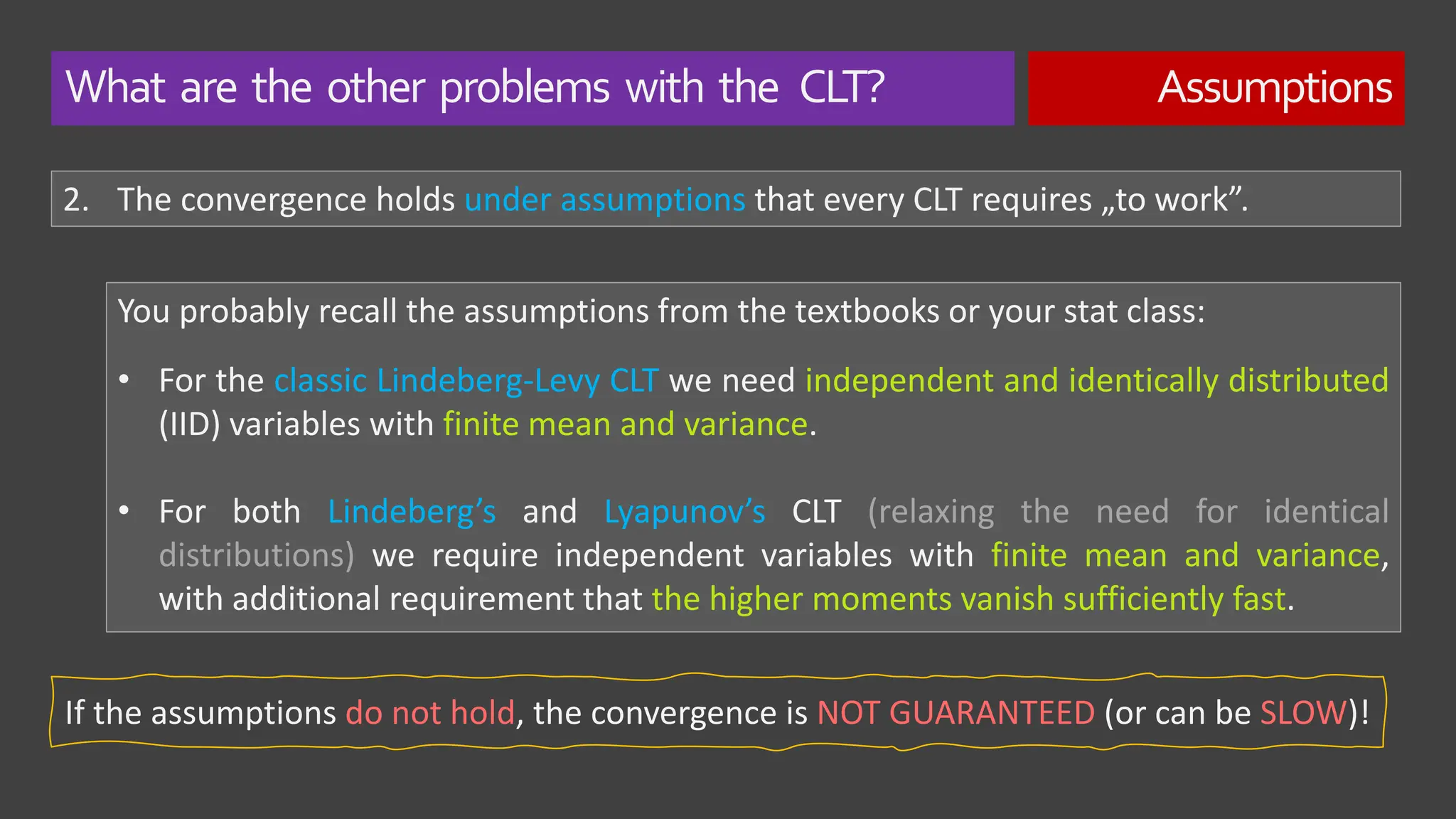
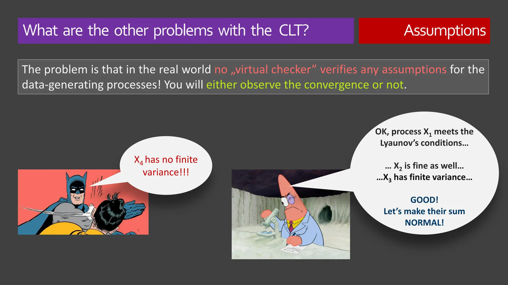
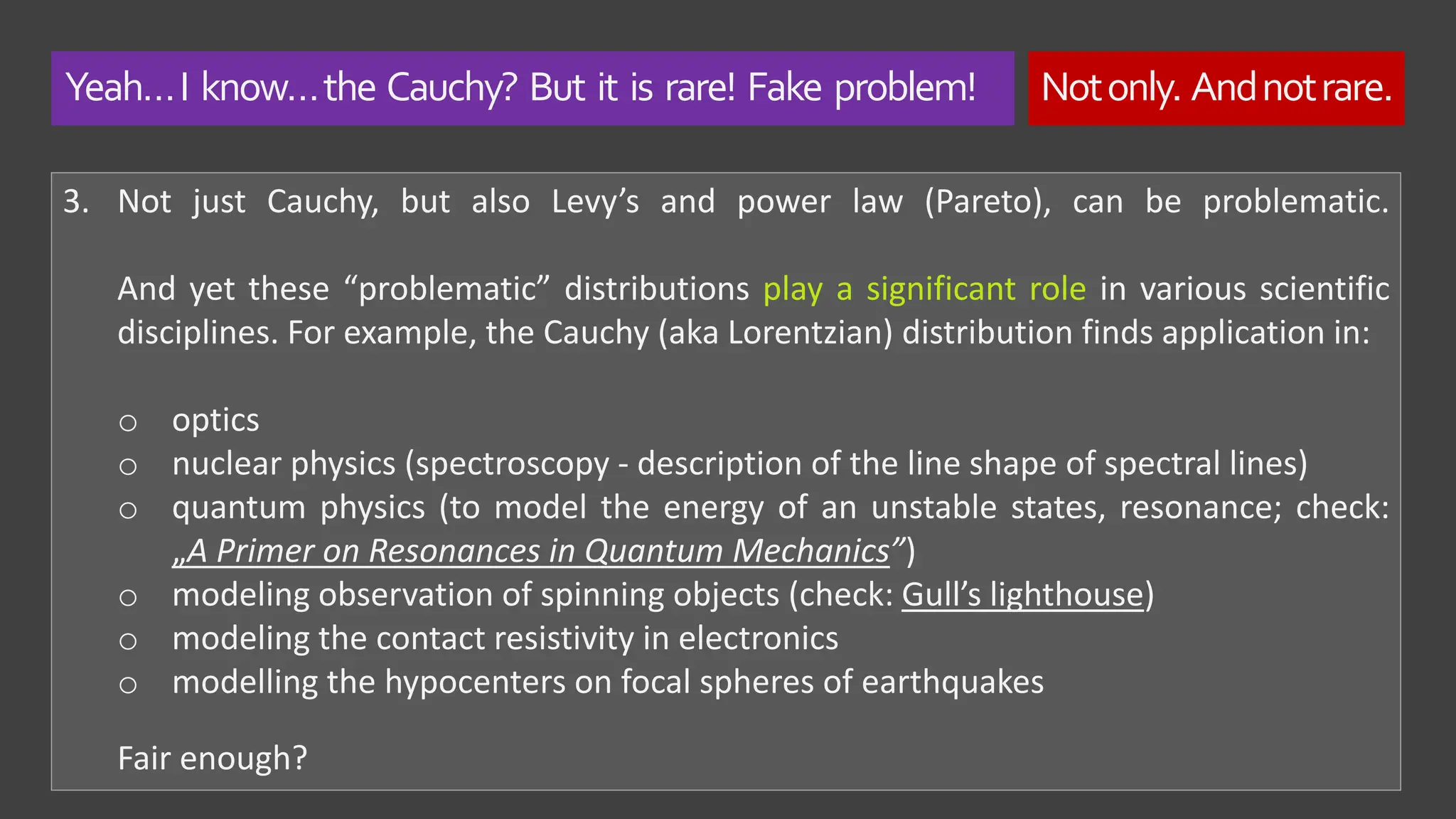
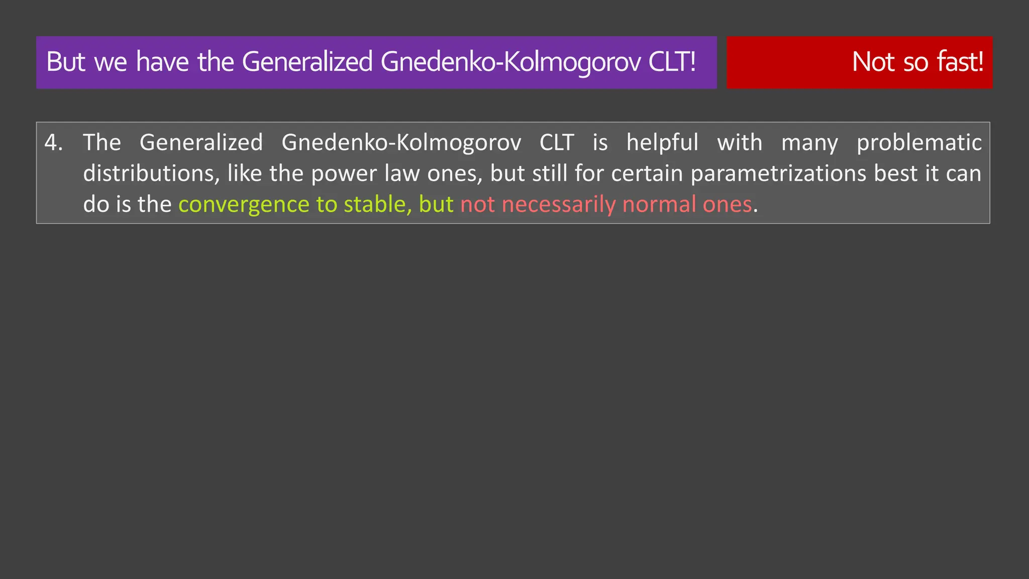
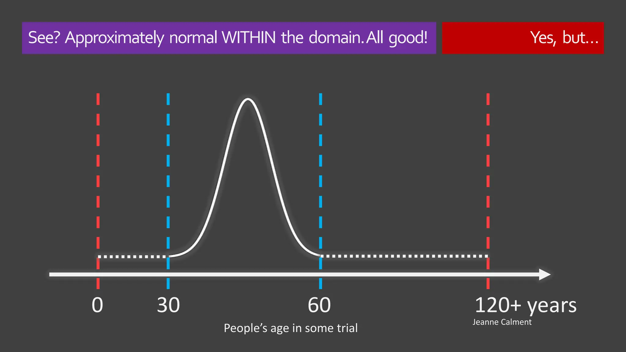
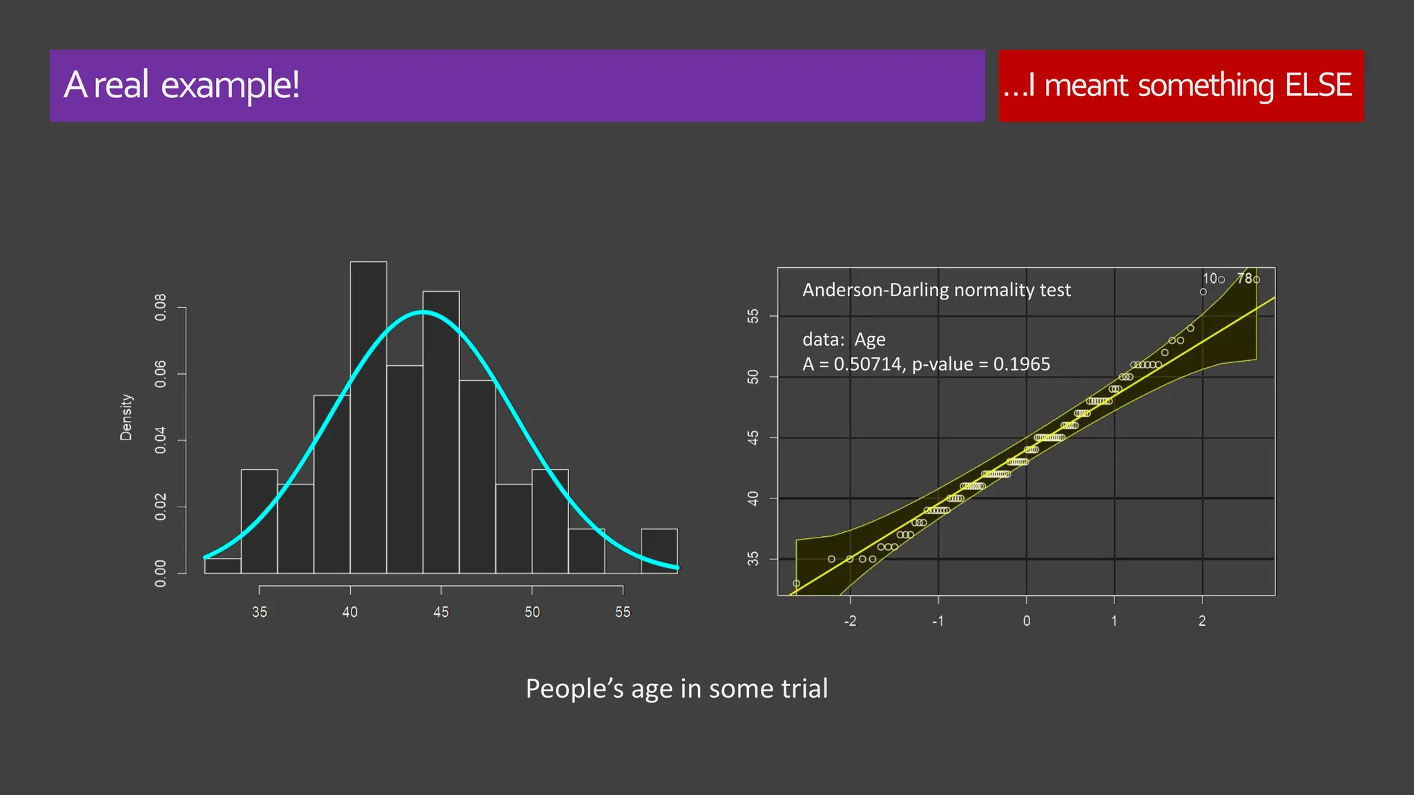
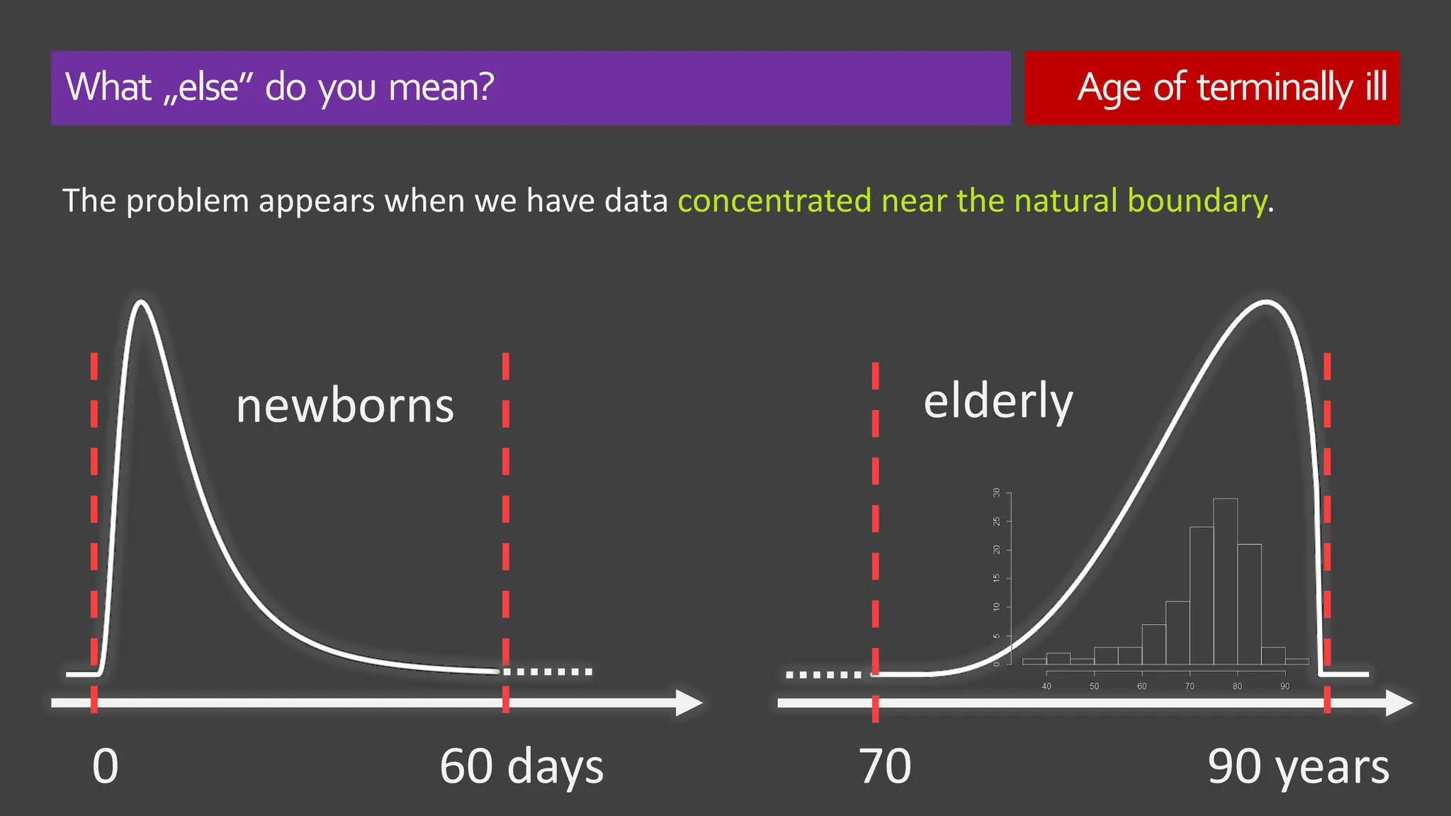
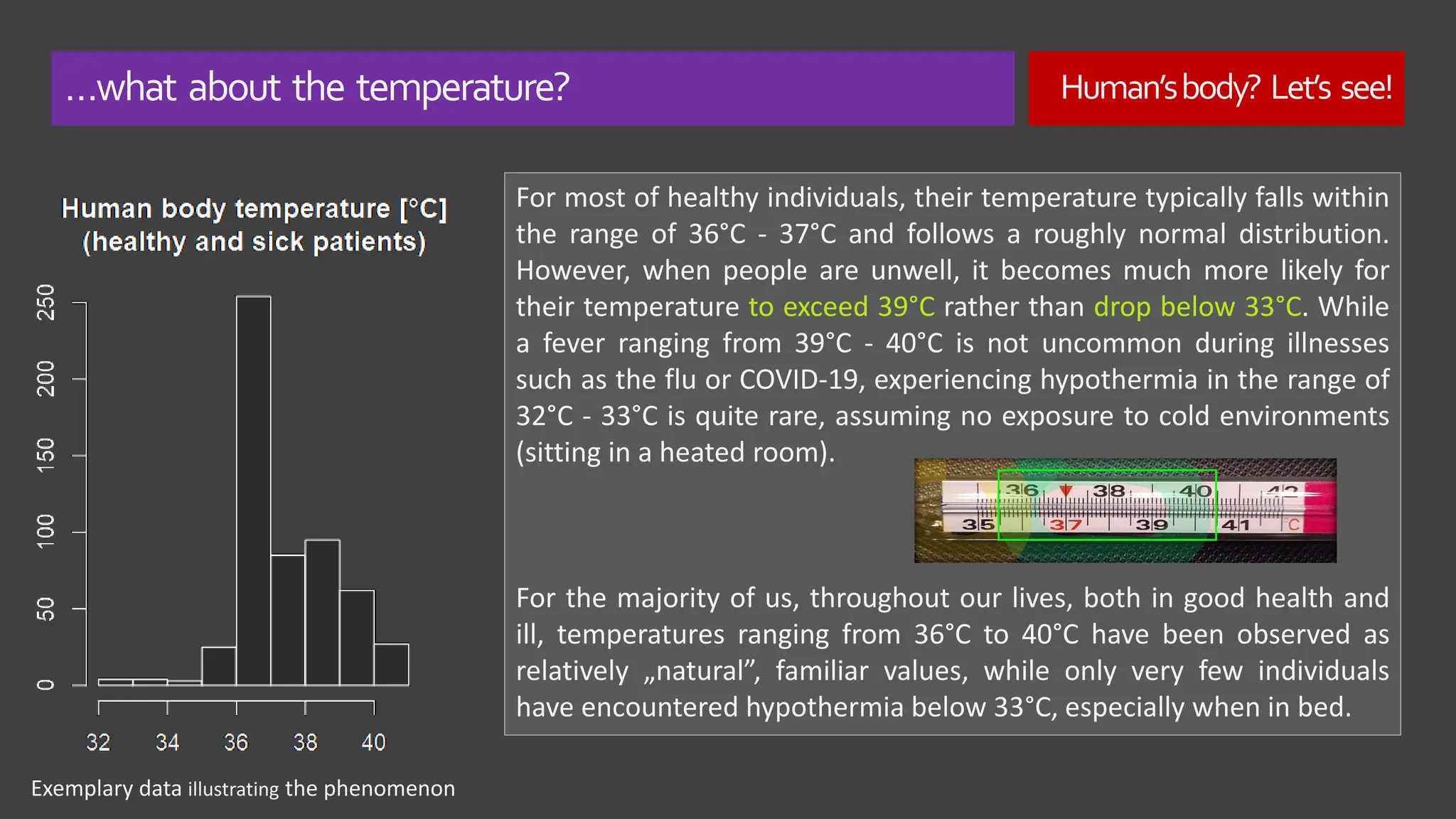
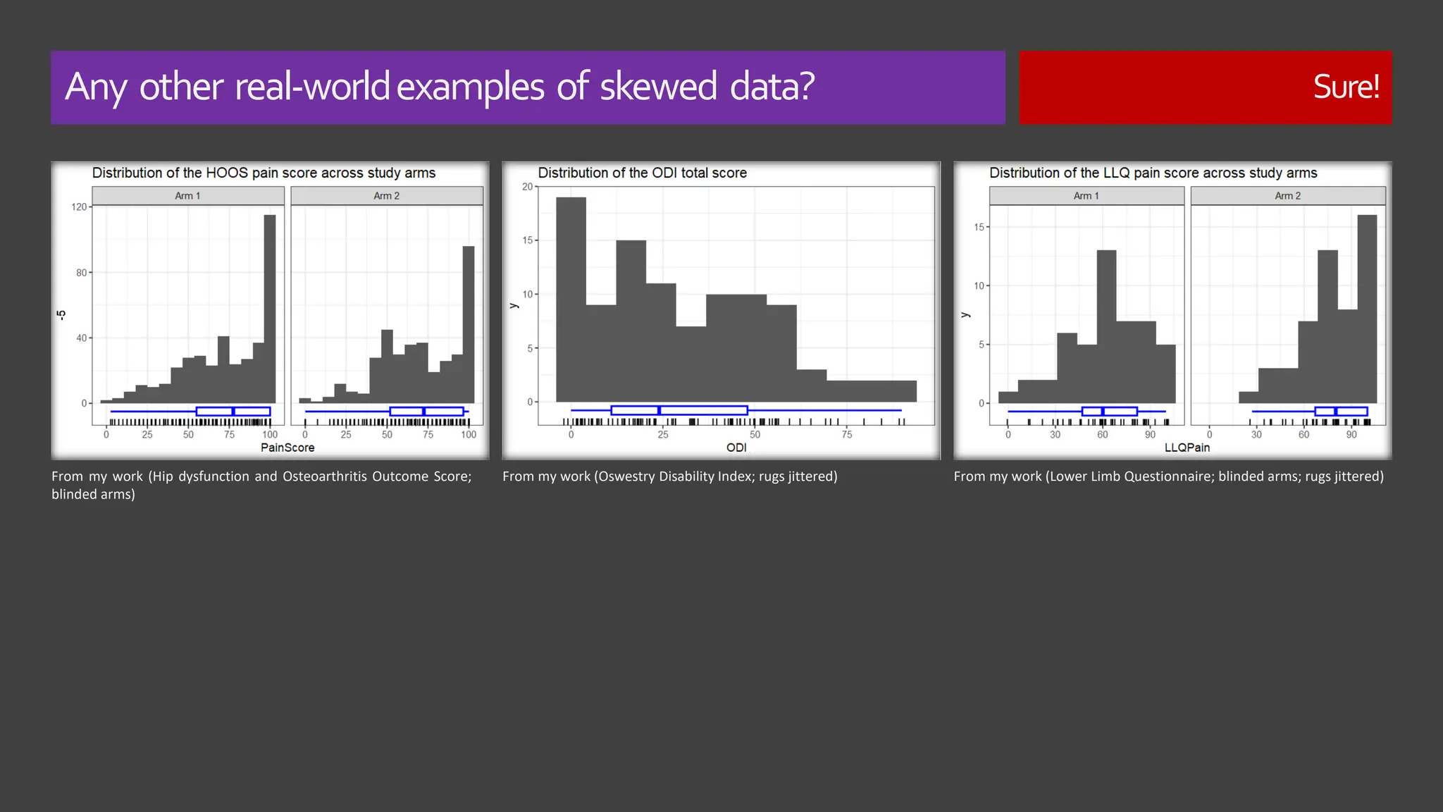
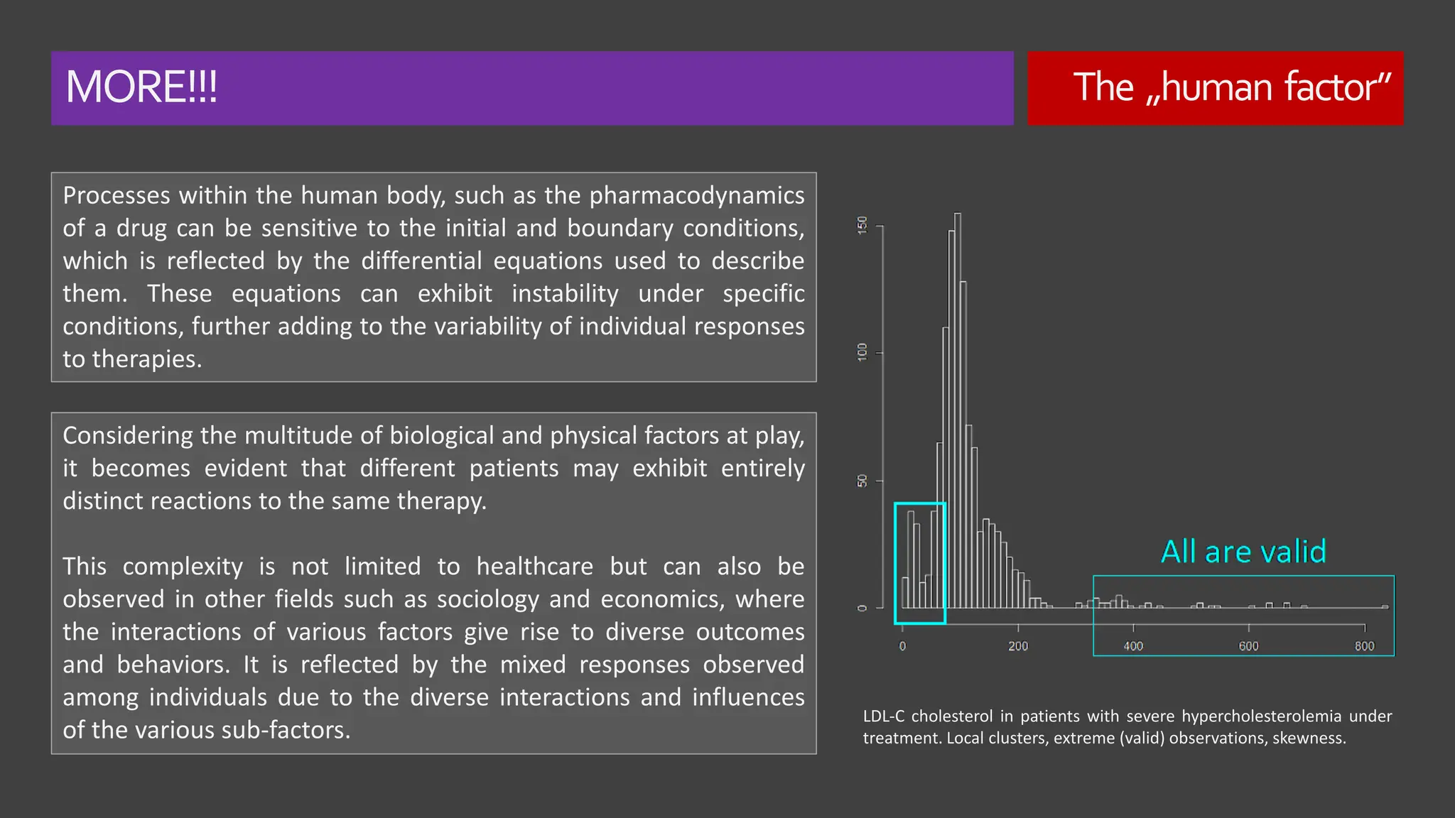
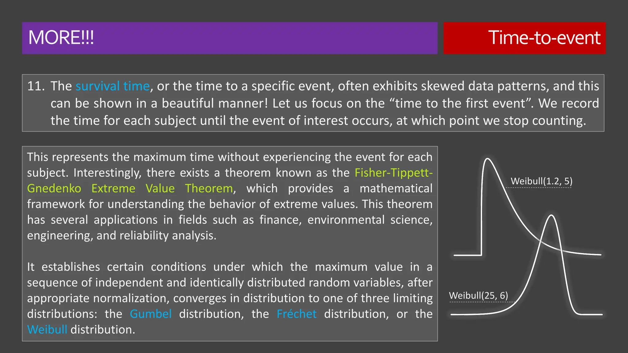
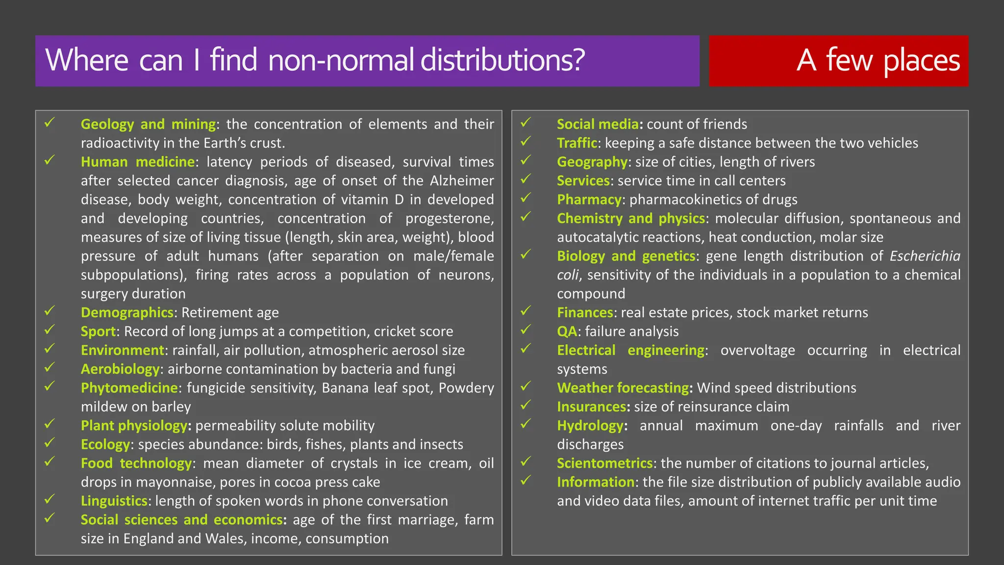
The document explores the concept of 'normality' in statistics, tracing its historical roots to Adolphe Quetelet and discussing the assumptions of the central limit theorem (CLT). It critiques the oversimplification of natural phenomena to normal distributions and highlights real-world examples of skewness and bounded features in data. Additionally, it examines the implications of multiplicative processes in various fields, emphasizing the need for rigorous consideration of CLT assumptions and their impact on data interpretation.

1. thecultofthe
normal distribution
inscience
Adrian Olszewski
and 2KMM CRO
The „challenging…” series in statistics with
in the Gaussian Distribution
we trust
challenging …
01.08.2023
Episode I

2. Quetilismus
The belief that “normality is everywhere”
has a long history that traces back to the
19th century and the work of
Adolphe Quetelet
Quetelet, a polymath who excelled in
various fields (mathematics, astronomy,
poetry, drama, and sociology) is
renowned as the inventor of the BMI.
He went much beyond the
Gaussian Theory of Errors and claimed
that normality is the default way of
describing world.

3. Quetilismus
There have been opponents of Quetelet’s
assumption that humanity can be
described by ’normal’ distributions.
Francis Edgeworth (1845–1926) said:
„The (Gaussian) theory of errors is to be
distinguished from the doctrine, the false
doctrine, that generally, wherever there is
a curve with a single apex representing a
group of statistics, that the curve must be
of the ’normal’ species".

4. It’s easy to echo easy explanations and generalizing one’s limited experience into global „laws”.
But one’s beliefs do not affect how the world actually „works”. One must embrace the facts.
People often call the Central Limit Theorem to justify their perspective. But they forget about many issues!
Additivity is NOT
enough
Assuming, that processes
act additively, i.e. what we
observe is a sum / mean of
actions is limiting,
What about the products
and mixtures of both?
CLT assumptions
do matter
All CLTs have their
assumptions for the
convergence-in-
distribution to happen.
What, if the assumptions
do NOT hold?
Bounded
features
Many real features
are naturally bounded
and concentrated
near the boundary.
We cannot ignore
this fact.
Natural sources
of skewness
The skewness can be
„derived” from physical
phenomena and equations
(1st-order kinetic equation,
increasing entropy),
Benford’s law
Mixtures of
distributions
Sometimes observed
data may be a mixture
of symmetrically
distributed features,
yet we do not know
how to separate them
meaningfully.
What do people „worshipping normality” usually miss?
ෑ
𝑖
𝑋𝑖
𝑑𝐶
𝑑𝑡
=-kC

5. ෑ
𝑖
𝑋𝑖
Additivity is NOT enough

6. The Central Limit Theorem explains it all! No. It does not.
Convolve
the PDFs
The Central Limit Theorem is commonly thought as a theorem about the distribution of means, but this is
equivalent to a convolution of the probability density functions. https://tinyurl.com/2ek5bfhw | https://tinyurl.com/2gt6o7t3
See? It
works!

7. You saw that it works, so what’s the problem? Additivity is not enough
1. The classic CLTs are additive - involve sums / averages of variables. By relying on that
one claims that the only way multiple processes can act together is the additive way.
But this is NOT TRUE. Processes can act multiplicatively and in both manners mixed.
/ that’s BTW why we have also the Multiplicative CLT; Google for the „Gibrat’s law” /
X1 X2 … Xn
Σ
X1 X2 … Xn
Π
X1 X2 … Xn
Σ Π
Σ/Π
… but Nature does not!
People usually stop here →

8. Why doesmultiplication cause skewness? Just by definition
When we add (subtract) a number to (from) a fixed value X, both sides of X are affected
equally, distanced from X by the same number of units. The results can be either positive
or negative, depending on the operation and the magnitude of the added value.
When we multiply (divide) a fixed value X by a number, the effect on both sides of X is not
equal. Dividing X by 2 halves it, while multiplying X by 2 doubles it. The effect of the
multiplication (or division) operation is then asymmetric. The sign is retained regardless of
the magnitude of the multiplier as long as it is positive.

9. So, when we take a product of multiple series of values… …it may get skewed
Summing series produces a new series in which the resulting values are symmetrically
scattered around a central value (mean or median). The occurrence of extreme values on
both sides of the distribution is approximately equal. When the series are independent,
the frequency of extreme values is expected to be smaller than the frequency of more
“typical” values. As the number of series increases, this distribution takes the familiar
shape we recognize as a “pyramid”, approaching the “bell curve”.
Multiplication of the series results in a new series where the resulting values exhibit
strong asymmetry around a ‘central’ value.

10. Show me! Here you are
Looks like the CLT at work!
and the Multiplicative CLT!

11. Tell me more! What kind of processes can act thisway? Forexample:
1. In biology, the skewness naturally arises through the ‘cascades of reactions’, where
metabolism and elimination processes can be described in multiplicative manner
because of combined activity of enzymes and hormones. Here the product of one
reaction serves as the substrate for another, or one hormone activates or inhibits the
production/release of another hormone(s). Skewed distributions are frequently
observed in pharmacokinetics, influenced by various physiological processes this way.
2. Levels of various biochemical markers, even if distributed approximately normally in
the population of healthy people, may exhibit extreme skewness in the population of
ill patients. The concentration of low-density lipoprotein cholesterol (LDL-C) in
patients under severe hypercholesterolemia or the levels of the PSA hormone in
oncological patients, (easily spanning 7 orders of magnitude in one direction).

12. Tell me more! What kind of processes can act thisway? For example:
Wosniok, Werner & Haeckel, Rainer. (2019). A new
indirect estimation of reference intervals:
truncated minimum chi-square (TMC) approach.
Clinical Chemistry and Laboratory Medicine
(CCLM). 57. 10.1515/cclm-2018-1341.
https://tinyurl.com/2ktyvd8c
Nunez, Derek & Alexander, Myriam & Yerges-
Armstrong, Laura & Singh, Gurparkash &
Byttebier, Geert & Fabbrini, Elisa & Waterworth,
Dawn & Meininger, Gary & Galwey, Nicholas &
Wallentin, Lars & White, Harvey &
Vannieuwenhuyse, Bart & Alazawi, William &
Kendrick, Stuart & Sattar, Naveed & Ferrannini,
Ele. (2018). Factors influencing longitudinal
changes of circulating liver enzyme
concentrations in subjects randomized to
placebo in four clinical trials. American Journal of
Physiology-Gastrointestinal and Liver Physiology.
316. 10.1152/ajpgi.00051.2018.
https://tinyurl.com/2o7svann
From my work
From my work
Brinkworth, Russell & Whitham,
Elaine & Nazeran, Homayoun. (2004).
Establishment of paediatric
biochemical reference intervals.
Annals of clinical biochemistry. 41.
321-9. 10.1258/0004563041201572.
https://tinyurl.com/2oj56b2f
From my work
Total bilirubin

13. BTW, can you show me the Multiplicative CLT at work? Sure!
Multiplied
Checked vs. normal after log-transformation ↗
Checked directly vs. log-normal →

14. CLT assumptions DO matter
ONE DOES NOT SIMPLY
IGNORE THE ASSUMPTIONS

15. What are the other problems with the CLT? Assumptions
2. The convergence holds under assumptions that every CLT requires „to work”.
You probably recall the assumptions from the textbooks or your stat class:
• For the classic Lindeberg-Levy CLT we need independent and identically distributed
(IID) variables with finite mean and variance.
• For both Lindeberg’s and Lyapunov’s CLT (relaxing the need for identical
distributions) we require independent variables with finite mean and variance,
with additional requirement that the higher moments vanish sufficiently fast.
If the assumptions do not hold, the convergence is NOT GUARANTEED (or can be SLOW)!

16. What are the other problems with the CLT? Assumptions
The problem is that in the real world no „virtual checker” verifies any assumptions for the
data-generating processes! You will either observe the convergence or not.
X4 has no finite
variance!!!
OK, process X1 meets the
Lyaunov’s conditions…
… X2 is fine as well…
…X3 has finite variance…
GOOD!
Let’s make their sum
NORMAL!

17. Yeah…I know…the Cauchy? But it is rare! Fake problem! Notonly. Andnotrare.
3. Not just Cauchy, but also Levy’s and power law (Pareto), can be problematic.
And yet these “problematic” distributions play a significant role in various scientific
disciplines. For example, the Cauchy (aka Lorentzian) distribution finds application in:
o optics
o nuclear physics (spectroscopy - description of the line shape of spectral lines)
o quantum physics (to model the energy of an unstable states, resonance; check:
„A Primer on Resonances in Quantum Mechanics”)
o modeling observation of spinning objects (check: Gull’s lighthouse)
o modeling the contact resistivity in electronics
o modelling the hypocenters on focal spheres of earthquakes
Fair enough?

18. But we have the Generalized Gnedenko-Kolmogorov CLT! Not so fast!
4. The Generalized Gnedenko-Kolmogorov CLT is helpful with many problematic
distributions, like the power law ones, but still for certain parametrizations best it can
do is the convergence to stable, but not necessarily normal ones.

19. Can you disappoint me even more? Sure ☺
Let’s do a completely free-ride,
employing the Lyapunov CLT. We define
5 types of symmetric & left/right
skewed distributions :
Uniform (min(1..10), max(1..10))
Beta (1..10, 1..10)
Gamma(1..10, 1..10)
logNormal(0.1..2, 0.1..2)
F(1..20, 1..20)
5 distributions were sampled with
replacement, centered, scaled, and
summed up. Parameters of these
distributions were sampled as well from
the listed ranges. The sampling was
repeated 20 times using different seeds.
The results contain both the histogram
with kernel estimator of the empirical
density, theoretical density of the
normal distribution (with parameters
estimated from the sample), Quantile-
Quantile plot, estimators of skewness
(should be 0) and Excess-Kurtosis
(should be 0) followed by the Shapiro-
Wilk test of non-normality.
The CLT did a great job, didn’t it!?

20. OK. Got the message… Fair enough? ☺
Oh no, I forgot to ONLY scale the variables 

21. Bounded features do exist in nature

22. What does it mean? Is this common inreal world? It’s very common
5. Lots of real physical phenomena result in naturally truncated (or bounded) variables:
o Truncated at one side (e.g. positive only): temperature (in Kelvin’s degrees),
weight, height, all dimensions and also distance, area, volume, speed (scalar),
time to some event, age, concentration (including all biochemical markers,
hormones, enzyme activity), frequency, amplitude, etc…
o Truncated at both sides: age (0-120 Jeanne Calment), adult’s weight (10kg-600kg Manuel Uribe)
And the normal distribution means the data can take any real value (also negative).
But that’s not a big problem. We could find the normal distribution describing the
data sufficiently well somewhere in the middle of the domain range.

23. See? Approximately normal WITHIN the domain.All good! Yes, but…
0 30 60 120+ years
People’s age in some trial
Jeanne Calment

24. Areal example! …I meant something ELSE
Anderson-Darling normality test
data: Age
A = 0.50714, p-value = 0.1965
People’s age in some trial

25. What „else” do you mean? Age of terminally ill
0 60 days
newborns
70 90 years
elderly
The problem appears when we have data concentrated near the natural boundary.

26. …what about the temperature? Human’sbody? Let’s see!
For most of healthy individuals, their temperature typically falls within
the range of 36°C - 37°C and follows a roughly normal distribution.
However, when people are unwell, it becomes much more likely for
their temperature to exceed 39°C rather than drop below 33°C. While
a fever ranging from 39°C - 40°C is not uncommon during illnesses
such as the flu or COVID-19, experiencing hypothermia in the range of
32°C - 33°C is quite rare, assuming no exposure to cold environments
(sitting in a heated room).
For the majority of us, throughout our lives, both in good health and
ill, temperatures ranging from 36°C to 40°C have been observed as
relatively „natural”, familiar values, while only very few individuals
have encountered hypothermia below 33°C, especially when in bed.
Exemplary data illustrating the phenomenon

27. Any other real-worldexamples of skewed data? Sure!
From my work (Hip dysfunction and Osteoarthritis Outcome Score;
blinded arms)
From my work (Oswestry Disability Index; rugs jittered) From my work (Lower Limb Questionnaire; blinded arms; rugs jittered)

28. Naturalsourcesofskewness
𝑑𝐶
𝑑𝑡
=-kC

29. Are there any other sources of skewness? Yes.Holdon.
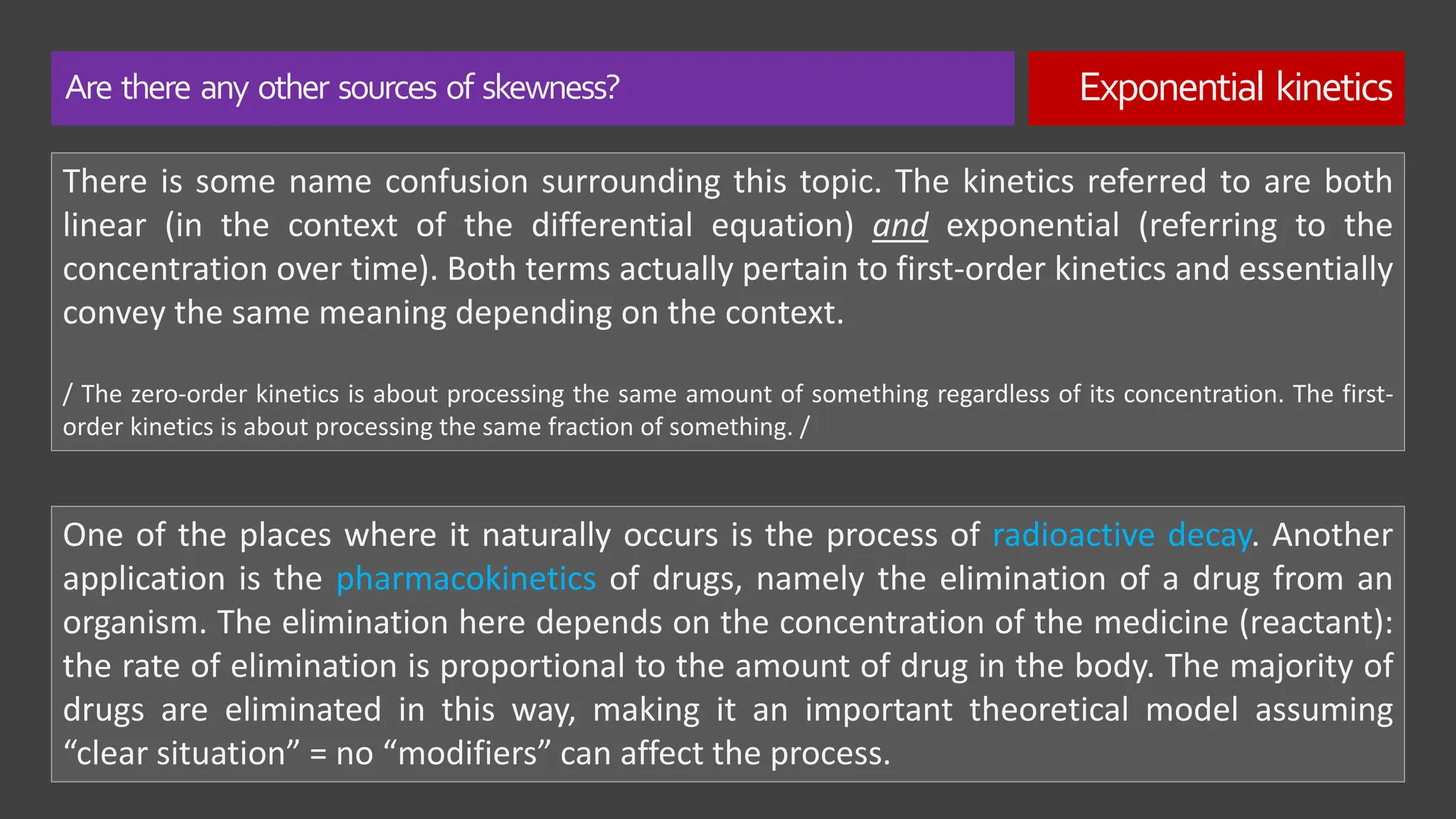
6. Exponential kinetics is a term describing a process, in which the rate of creating
(concentrating) or losing some substance or property is proportional to the remaining
amount of the substance. A constant proportion (not amount!) of something is
processed per unit time. Or differently - the greater the amount of something, the
faster the process.
𝑑𝐶
𝑑𝑡
= −kC [1]
Because of the exponential form of the solution to the above equation:
The process is called “mono-exponential rate process” and represents exponential
decay or concentration over time.
𝐶 = 𝐶0𝑒−𝑘𝑡 [2]

30. Are there any other sources of skewness? Exponential kinetics
There is some name confusion surrounding this topic. The kinetics referred to are both
linear (in the context of the differential equation) and exponential (referring to the
concentration over time). Both terms actually pertain to first-order kinetics and essentially
convey the same meaning depending on the context.
/ The zero-order kinetics is about processing the same amount of something regardless of its concentration. The first-
order kinetics is about processing the same fraction of something. /
One of the places where it naturally occurs is the process of radioactive decay. Another
application is the pharmacokinetics of drugs, namely the elimination of a drug from an
organism. The elimination here depends on the concentration of the medicine (reactant):
the rate of elimination is proportional to the amount of drug in the body. The majority of
drugs are eliminated in this way, making it an important theoretical model assuming
“clear situation” = no “modifiers” can affect the process.

31. Are there any other sources of skewness? Exponential kinetics
While k = const is reasonable for the radioactive decay (allowing us to calculate the half-
life: t½≈0.693/k), the elimination of drugs may strongly depend on many factors:
interactions with other drugs and human factor (described earlier sum-product of many
factors). In this case, the constant “k” may vary. And then the equation [1] turns into a
stochastic differential equation:
𝑑 𝑋
𝑑𝑡
= −(𝜇𝑘 + 𝜎𝑘𝜂(𝑡))[𝑋] [3]
where μk is the mean reaction rate and σk is the magnitude of the stochastic fluctuation.
The function η(t) describes the time-dependency of the random fluctuations (with
amplitude 1), which we here assume to be independent and identically normally
distributed. Fluctuations of η(t) will result in fluctuations of the solution for the equation
[3], which creates a random variable. Now HOLD ON!

32. Are there any other sources of skewness? Exponential kinetics
The equation that describes the temporal evolution of the PDF of this variable is the
Fokker–Planck equation. It turns out, that the solution of the Fokker-Planck equation
derived from the equation [3] is the PDF of the log-normal distribution!
Briefly, the first-order kinetic model with
randomly fluctuating sink/concentration rate is
a potential source of the log-normality in
nature. Isn’t this beautiful😍?
Think how widespread is this mechanism in
physics, chemistry, biology!

33. Where can I read more about this phenomenon? Here:
• Shen M., Russek-Cohen E. & Slud E. V. (2016):Checking distributional assumptions for pharmacokinetic
summary statistics based onsimulations with compartmental models, Journal of Biopharmaceutical
Statistics, DOI:10.1080/10543406.2016.1222535,
https://www.math.umd.edu/~slud/myr.html/PharmStat/JBSpaper2016.pdf
• https://en.wikipedia.org/wiki/Fokker%E2%80%93Planck_equation
• Andersson, A. Mechanisms for log normal concentration distributions in the environment. Sci Rep 11,
16418 (2021). https://doi.org/10.1038/s41598-021-96010-6, https://www.nature.com/articles/s41598-
021-96010-6

34. I want more! Multi-agent systems
7. What if I told you that similar mechanisms are much more widespread in kinetics
theory in social sciences and economics? The above-mentioned Fokker-Planck-type
equations naturally link with the theory of multi-agent systems, used to describe
human activities and economic phenomena.
Let’s consider a certain specific hallmark of the population of agents. The hallmark is
measured in terms of some positive value “w”. The agents have the objective to reach a
target fixed value of “w” by repeated upgrading. This corresponds to microscopic
interactions. The upgrade of the actual value towards the target is different, depending
on the actual state of the agents, it’s dynamic. This leads to the same problem and a
similar solution to the described in the previous section!
Gualandi S., Toscani G., Human behavior and lognormal distribution. A kinetic description, Mathematical
Models and Methods in Applied Sciences 2019 29:04, 717-753, https://arxiv.org/abs/1809.01365

35. MORE!!! Increasing entropy
8. Another way to infer log-normality from fundamental laws is to refer to entropy.
Fluctuations in open-system processes (exchanging both energy and matter with its
surroundings) in their evolution toward more probable states yield multiplicative
variations about the mean. The non-linear dispersion of thermodynamic states, i.e.
matter and energy defined by chemical potentials, underlies the skewness.
Details can be found in the following article, where the authors call the log-normal
distribution the “Natural Distribution”, coming from physical processes with
conserved positive quantities:
Grönholm T, Annila A. Natural distribution. Math Biosci. 2007;210(2):659-667.
doi:10.1016/j.mbs.2007.07.004, https://www.mv.helsinki.fi/home/aannila/arto/naturaldistribution.pdf

36. MORE!!! The Benford’s Law
9. Benford’s Law is a fascinating phenomenon that exemplifies the presence of skewness
in real-world datasets. It observes that in various collections of numbers – such as
mathematical tables, real-life data, or their combinations – the leading significant
digits do not exhibit a uniform distribution as expected, but instead display a strong
skewness towards the smaller digits. Benford’s Law states that the significant digits in
many datasets follow a log-normal distribution.
This law has numerous applications, including fraud
detection, criminal investigations, social media analysis,
genome data analysis, financial investigations, and
macroeconomic data analysis, among others. It is
important to note that there are also significant counter-
applications of Benford’s Law, such as its use in analyzing
election data under specific conditions.
Distribution of first digits (in %, red bars)
in the population of the 237 countries of
the world as of July 2010. Black dots
indicate the distribution predicted by
Benford’s law. (source Wikipedia)

37. MORE!!! The Benford’s Law
• Berger, A., Hill, T.P. Benford’s Law Strikes Back: No Simple Explanation in Sight for
Mathematical Gem. Math Intelligencer 33, 85–91 (2011).
https://doi.org/10.1007/s00283-010-9182-3,
https://digitalcommons.calpoly.edu/cgi/viewcontent.cgi?referer=https://en.wikipedia
.org/&httpsredir=1&article=1074&context=rgp_rsr
• Miller, S. (2015). Benford's Law: Theory and Applications.
https://www.researchgate.net/publication/280157559_Benford%27s_Law_Theory_a
nd_Applications
• Gonsalves R. A., Benford’s Law — A Simple Explanation,
https://towardsdatascience.com/benfords-law-a-simple-explanation-341e17abbe75
Another illustration of the
Benford's law
(source Wikipedia)

38. MORE!!! The „human factor”
10. The individual “human factor” introduces a significant level of unpredictability and
leads to diverse responses to treatment among patients. When analyzing data from
patients collectively, we often observe a wide range of patterns, including multiple
modes, strong skewness, and extreme (valid!) outliers.
The complexity of the “human factor” arises from a multitude of interconnected sub-factors. Thousands of chemical
reactions occur within our bodies every second, and any disruptions or failures in these reactions can have an impact.
Furthermore, numerous environmental conditions such as temperature, humidity, air pressure, and pollution can
influence our physiological responses.
Personal habits, including smoking and drinking, dietary choices, hydration status, medications and their interactions,
surgical procedures, illnesses, infections, allergies, deficiencies, and overdosing of drugs all contribute to the intricate
web of factors affecting our health. Additionally, our DNA and its mutations, which can be caused by factors like
radiation and mutagens present in our environment (such as carcinogenic substances in food and water), have a
significant influence. Hormonal and enzymatic activity, stress levels, lifestyle (ranging from sedentary to highly active /
extreme), familial burdens, and even the placebo / nocebo effects add further complexity.

39. MORE!!! The „human factor”
Processes within the human body, such as the pharmacodynamics
of a drug can be sensitive to the initial and boundary conditions,
which is reflected by the differential equations used to describe
them. These equations can exhibit instability under specific
conditions, further adding to the variability of individual responses
to therapies.
LDL-C cholesterol in patients with severe hypercholesterolemia under
treatment. Local clusters, extreme (valid) observations, skewness.
Considering the multitude of biological and physical factors at play,
it becomes evident that different patients may exhibit entirely
distinct reactions to the same therapy.
This complexity is not limited to healthcare but can also be
observed in other fields such as sociology and economics, where
the interactions of various factors give rise to diverse outcomes
and behaviors. It is reflected by the mixed responses observed
among individuals due to the diverse interactions and influences
of the various sub-factors.

40. MORE!!! Time-to-event
11. The survival time, or the time to a specific event, often exhibits skewed data patterns, and this
can be shown in a beautiful manner! Let us focus on the “time to the first event”. We record
the time for each subject until the event of interest occurs, at which point we stop counting.
This represents the maximum time without experiencing the event for each
subject. Interestingly, there exists a theorem known as the Fisher-Tippett-
Gnedenko Extreme Value Theorem, which provides a mathematical
framework for understanding the behavior of extreme values. This theorem
has several applications in fields such as finance, environmental science,
engineering, and reliability analysis.
It establishes certain conditions under which the maximum value in a
sequence of independent and identically distributed random variables, after
appropriate normalization, converges in distribution to one of three limiting
distributions: the Gumbel distribution, the Fréchet distribution, or the
Weibull distribution.
Weibull(1.2, 5)
Weibull(25, 6)

41. MORE!!! Time-to-event
The Fisher-Tippett-Gnedenko Extreme Value Theorem does not claim that the normalized
maximum values eventually converge in distribution, BUT if they do, the limiting
distribution is either of the three mentioned above.
/ By the way, when the shape parameter of the Weibull distribution is set to 3, it closely resembles the normal
distribution /
This does not end the list! Exponential, gamma, log-normal, and log-logistic distributions
are other (potentially) skewed distributions commonly used in the time-to-event analysis
as well.

42. Mixturesofdistributions

43. What about the mixtures of distributions? They existandmatter
12. Mixtures of distributions can naturally form skewness. A typical example is a mixture of (approximate)
normal distributions with some mean-variance relationship, typically – the larger the mean the larger
the variance. In some cases, mixtures can be effectively separated during the analysis. If analysts have
prior domain knowledge suggesting the presence of a discriminatory categorical factor, they can
include this factor as a covariate in their model. By doing so, the mixture can be divided into
approximately symmetric and homogeneous groups.
This provides an explanation for the emergence of a virtual skewness in the data, which can occur when
certain factors that could potentially differentiate groups are overlooked. Frequently, we may not even be
aware that such factors exist, leading to the treatment of inseparable mixtures as a single entity.
We will observe such case on the next slide.

44. What about the mixtures of distributions? They existandmatter
Sikaris, Kenneth A.. "Separating disease and health for indirect
reference intervals" Journal of Laboratory Medicine, vol. 45, no.
2, 2021, pp. 55-68. https://doi.org/10.1515/labmed-2020-0157
https://tinyurl.com/2g47qps8
When you know the
separation factor
When you do NOT know
the separation factor
There are three samples sampled from the normal distributions of different location and spread form. The three
distributions were mixed (not summed!) and form a skewed one on the right. With no prior knowledge about the
„components” and the separating factor(s), in nature we will observe just a skewed distribution.

45. Someplaceswithnatural presence ofskewness

46. Where can I find non-normaldistributions? A few places
✓ Geology and mining: the concentration of elements and their
radioactivity in the Earth’s crust.
✓ Human medicine: latency periods of diseased, survival times
after selected cancer diagnosis, age of onset of the Alzheimer
disease, body weight, concentration of vitamin D in developed
and developing countries, concentration of progesterone,
measures of size of living tissue (length, skin area, weight), blood
pressure of adult humans (after separation on male/female
subpopulations), firing rates across a population of neurons,
surgery duration
✓ Demographics: Retirement age
✓ Sport: Record of long jumps at a competition, cricket score
✓ Environment: rainfall, air pollution, atmospheric aerosol size
✓ Aerobiology: airborne contamination by bacteria and fungi
✓ Phytomedicine: fungicide sensitivity, Banana leaf spot, Powdery
mildew on barley
✓ Plant physiology: permeability solute mobility
✓ Ecology: species abundance: birds, fishes, plants and insects
✓ Food technology: mean diameter of crystals in ice cream, oil
drops in mayonnaise, pores in cocoa press cake
✓ Linguistics: length of spoken words in phone conversation
✓ Social sciences and economics: age of the first marriage, farm
size in England and Wales, income, consumption
✓ Social media: count of friends
✓ Traffic: keeping a safe distance between the two vehicles
✓ Geography: size of cities, length of rivers
✓ Services: service time in call centers
✓ Pharmacy: pharmacokinetics of drugs
✓ Chemistry and physics: molecular diffusion, spontaneous and
autocatalytic reactions, heat conduction, molar size
✓ Biology and genetics: gene length distribution of Escherichia
coli, sensitivity of the individuals in a population to a chemical
compound
✓ Finances: real estate prices, stock market returns
✓ QA: failure analysis
✓ Electrical engineering: overvoltage occurring in electrical
systems
✓ Weather forecasting: Wind speed distributions
✓ Insurances: size of reinsurance claim
✓ Hydrology: annual maximum one-day rainfalls and river
discharges
✓ Scientometrics: the number of citations to journal articles,
✓ Information: the file size distribution of publicly available audio
and video data files, amount of internet traffic per unit time

47. Literature

48. Where can I read more? A few proposals
Geology and mining
Singer D. A., The lognormal distribution of metal resources in mineral deposits, Ore Geology Reviews, Volume 55, 2013, Pages 80-86, ISSN 0169-
1368, https://doi.org/10.1016/j.oregeorev.2013.04.009, https://www.sciencedirect.com/science/article/pii/S0169136813001133
Biology and biophysics
Furusawa C, Suzuki T, Kashiwagi A, Yomo T, Kaneko K. Ubiquity of log-normal distributions in intra-cellular reaction dynamics. Biophysics
(Nagoya-shi). 2005 Apr 21;1:25-31. doi: 10.2142/biophysics.1.25. PMID: 27857550; PMCID: PMC5036630.
https://www.ncbi.nlm.nih.gov/pmc/articles/PMC5036630/
D.Fraga, K.Stock, M.Aryal, et al., Bacterial arginine kinases have a highly skewed distribution within the proteobacteria, Comparative
Biochemistry and Physiology, (2019), Part B, https://doi.org/10.1016/j.cbpb.2019.04.001,
https://www.sciencedirect.com/science/article/abs/pii/S1096495919300831?via%3Dihub
Epidemiology
Saltzman BE. Lognormal model for determining dose-response curves from epidemiological data and for health risk assessment [published
correction appears in Appl Occup Environ Hyg 2001 Oct;16(10):991]. Appl Occup Environ Hyg. 2001;16(7):745-754.
doi:10.1080/10473220121485, https://pubmed.ncbi.nlm.nih.gov/11458922/
Stock market
I. Antoniou, Vi.V Ivanov, Va.V Ivanov, P.V Zrelov, On the log-normal distribution of stock market data, Physica A: Statistical Mechanics and its
Applications, Volume 331, Issues 3–4, 2004,Pages 617-638, ISSN 0378-4371, https://doi.org/10.1016/j.physa.2003.09.034

49. Where can I read more? A few proposals
Pharmaceutical industry
Meiyu Shen, Estelle Russek-Cohen & Eric V. Slud (2016): Checking distributional assumptions for pharmacokinetic summary statistics based
onsimulations with compartmental models, Journal of Biopharmaceutical Statistics, DOI:10.1080/10543406.2016.1222535
Lacey LF, Keene ON, Pritchard JF, Bye A. Common noncompartmental pharmacokinetic variables: are they normally or log-normally distributed?.
J Biopharm Stat. 1997;7(1):171-178. doi:10.1080/10543409708835177
Clinical biochemistry and laboratory diagnostics
Feldman M, Dickson B. Plasma Electrolyte Distributions in Humans-Normal or Skewed?. Am J Med Sci. 2017;354(5):453-457.
doi:10.1016/j.amjms.2017.07.012, https://pubmed.ncbi.nlm.nih.gov/29173354/
Campbell D J, Hull E.W., Does serum cholesterol distribution have a log- normal component?
Kletzky OA, Nakamura RM, Thorneycroft IH, Mishell DR Jr. Log normal distribution of gonadotropins and ovarian steroid values in the normal
menstrual cycle. Am J Obstet Gynecol. 1975;121(5):688-694. doi:10.1016/0002-9378(75)90474-3
Distler W, Stollenwerk U, Morgenstern J, Albrecht H. Log normal distribution of ovarian and placental steroid values in early human pregnancy.
Arch Gynecol. 1978;226(3):217-225. doi:10.1007/BF02108902

50. Where can I read more? A few proposals
Ecology & Environment
Ogana, F. & Danladi W. (2018). Comparison of Gamma, Lognormal and Weibull Functions for Characterising Tree Diameters in Natural Forest.
Cho, H., Bowman, K. P., & North, G. R. (2004). A Comparison of Gamma and Lognormal Distributions for Characterizing Satellite Rain Rates from
the Tropical Rainfall Measuring Mission, Journal of Applied Meteorology, 43(11), 1586-1597. Retrieved Jun 29, 2022, from
https://journals.ametsoc.org/view/journals/apme/43/11/jam2165.1.xml
Jaci, Ross Joseph, "The gamma distribution as an alternative to the lognormal distribution in environmental applications" (2000). UNLV
Retrospective Theses & Dissertations. 1206. http://dx.doi.org/10.25669/z0ze-k42y ,
https://digitalscholarship.unlv.edu/cgi/viewcontent.cgi?article=2205&context=rtds
Sociology
Yook, S. H., & Kim, Y. (2020). Origin of the log-normal popularity distribution of trending memes in social networks. Physical Review E, 101(1),
[012312]. https://doi.org/10.1103/PhysRevE.101.012312
Physics
Grönholm T, Annila A. Natural distribution. Math Biosci. 2007;210(2):659-667. doi:10.1016/j.mbs.2007.07.004,
https://www.mv.helsinki.fi/home/aannila/arto/naturaldistribution.pdf

51. Where can I read more? A few proposals
Interdisciplinary
Andersson, A. Mechanisms for log normal concentration distributions in the environment. Sci Rep 11, 16418 (2021).
https://doi.org/10.1038/s41598-021-96010-6, https://www.nature.com/articles/s41598-021-96010-6
Limpert E., Stahel W. A., Abbt M., Log-normal Distributions across the Sciences: Keys and Clues: On the charms of statistics, and how mechanical
models resembling gambling machines offer a link to a handy way to characterize log-normal distributions, which can provide deeper insight
into variability and probability—normal or log-normal: That is the question, BioScience, Volume 51, Issue 5, May 2001, Pages 341–352,
https://doi.org/10.1641/0006-3568(2001)051[0341:LNDATS]2.0.CO;2 , https://stat.ethz.ch/~stahel/lognormal/bioscience.pdf
Gonsalves R. A., Benford’s Law — A Simple Explanation, https://towardsdatascience.com/benfords-law-a-simple-explanation-341e17abbe75

52. That’sall,folks!
I am wondering if – after reading this presentation - you will now look differently at the
widespread belief that skewness is something marginal or even bad, and that everything
should follow a normal distribution. Nobody denies, that the normal distribution is
extremely useful in both theoretical and applied statistics.
But now you know that skewness is no less common in nature and can be derived even
from physical principles.

53. Adrian Olszewski
clinical biostatistician at 2KMM CRO
https://www.2kmm.pl
https://www.linkedin.com/in/adrianolszewski/
Visit our blog at:
https://www.2kmm.pl/blog/