Download to read offline


![6
BETA DISTRIBUTION
Copyright © 2020, DexLab Solutions Corporation
BETA DISTIBUTION
In probability theory and statistics, the beta distribution is a family of continuous probability distributions defined on the interval [0, 1] parameterized by two positive shape
parameters, denoted by α and β, that appear as exponents of the random variable and control the shape of the distribution.
The beta distribution has been applied to model the behaviour of random variables limited to intervals of finite length in a wide variety of disciplines.
Probability Density Function for Beta Distribution
The probability density function (PDF) of the beta distribution, for 0 ≤ x ≤ 1, and shape parameters α, β > 0, is a power function of the variable x and of its reflection (1 − x) as
follows:
𝒇 𝒙; 𝜶, 𝜷 = 𝑪𝒐𝒏𝒔𝒕𝒂𝒏𝒕. 𝒙 𝜶−𝟏(𝟏 − 𝒙) 𝜷−𝟏
=
𝒙 𝜶−𝟏(𝟏 − 𝒙) 𝜷−𝟏
𝟎
𝟏
𝒖 𝜶−𝟏(𝟏 − 𝒖) 𝜷−𝟏 𝒅𝒖
=
Ґ(𝜶 + 𝜷)
Ґ 𝜶 Ґ(𝜷)
𝒙 𝜶−𝟏(𝟏 − 𝒙) 𝜷−𝟏=
𝟏
𝑩(𝜶, 𝜷)
𝒙 𝜶−𝟏(𝟏 − 𝒙) 𝜷−𝟏
Where Γ(z) is the gamma function. The beta function, B, =+is a normalization constant to ensure
that the total probability integrates to 1. In the above equations x is a realization—an observed
value that actually occurred—of a random process X.
This definition includes both ends x = 0 and x = 1, which is consistent with the definitions for other
continuous distributions supported on a bounded interval which are special cases of the beta
distribution, for example the arcsine distribution, and consistent with several authors, like
N. L. Johnson and S. Kotz. However, the inclusion of x = 0 and x = 1 does not work for α, β < 1;
accordingly, several other authors, including W. Feller, choose to exclude the ends x = 0 and
x = 1, (so that the two ends are not actually part of the domain of the density function) and
consider instead 0 < x < 1. Several authors, including N. L. Johnson and S. Kotz, use the
symbols p and q (instead of α and β) for the shape parameters of the beta distribution,
reminiscent of the symbols are traditionally used for the parameters of the Bernoulli distribution,
because the beta distribution approaches the Bernoulli distribution in the limit when both
shape parameters α and β approach the value of zero.
In the following, a random variable X beta-distributed with parameters α and β will be denoted by:
𝑋~𝐵𝑒𝑡𝑎(𝛼, 𝛽)
Other notations for beta-distributed random variables used in the statistical literature are 𝑋 − 𝐵𝑒 𝛼, 𝛽 𝑎𝑛𝑑 𝑋~𝛽 𝛼,𝛽.
Moment Generating Function for Beta Distribution
The moment generating function 𝑀 𝑋 of X is given by: 𝑀 𝑋 𝑡 = 1 + 𝑘=1
∞
𝑟=0
𝑘−1 𝛼+𝑟
𝛼+𝛽+𝑟
𝑡 𝑘
𝑘!
From the definition of a moment generating function: 𝑀 𝑋 𝑡 = 𝐸 𝑒 𝑡𝑥 = 0
1
𝑒 𝑡𝑥 𝑓𝑋(𝑥) . 𝑑𝑥
So: 𝑀 𝑋 𝑡 =
1
𝐵 𝛼,𝛽 0
1
𝑒 𝑡𝑥 𝑥 𝛼−1 1 − 𝑥 𝛽−1 𝑑𝑥 =
1
𝐵 𝛼,𝛽 0
1
𝑘=0
∞ 𝑡𝑥 𝑘
𝑘!
𝑥 𝛼−1 1 − 𝑥 𝛽−1 𝑑𝑥
=
𝑘=1
∞
𝑡 𝑘
𝑘!
𝐵 𝛼 + 𝐾, 𝛽
𝐵 𝛼, 𝛽
=
𝐵(𝛼, 𝛽)𝑡0
𝐵 𝛼, 𝛽 0!
+
𝑘=1
∞
𝑡 𝑘
𝑘!
𝐵 𝛼 + 𝑘, 𝛽
𝐵 𝛼, 𝛽
= 1 +
𝑘=1
∞
𝛤(∞) 𝑟=0
𝑘
(𝛼 + 𝑟)
𝛤(𝛼)
.
𝛤 𝛼 + 𝛽
𝛤 𝛼 + 𝛽 𝑟=0
𝑘
𝛼 + 𝛽 + 𝑟
𝑡 𝑘
𝑘!
= 1 +
𝑘=1
∞
𝑟=0
𝑘−1 𝛼 + 𝑟
𝛼 + 𝛽 + 𝑟
𝑡 𝑘
𝑘!](https://image.slidesharecdn.com/dexlabbasicsofstatisticalinferencepartiitypesofsamplingdistribution24062020v1reviewed-200708095944/75/Statistical-Inference-Part-II-Types-of-Sampling-Distribution-6-2048.jpg)


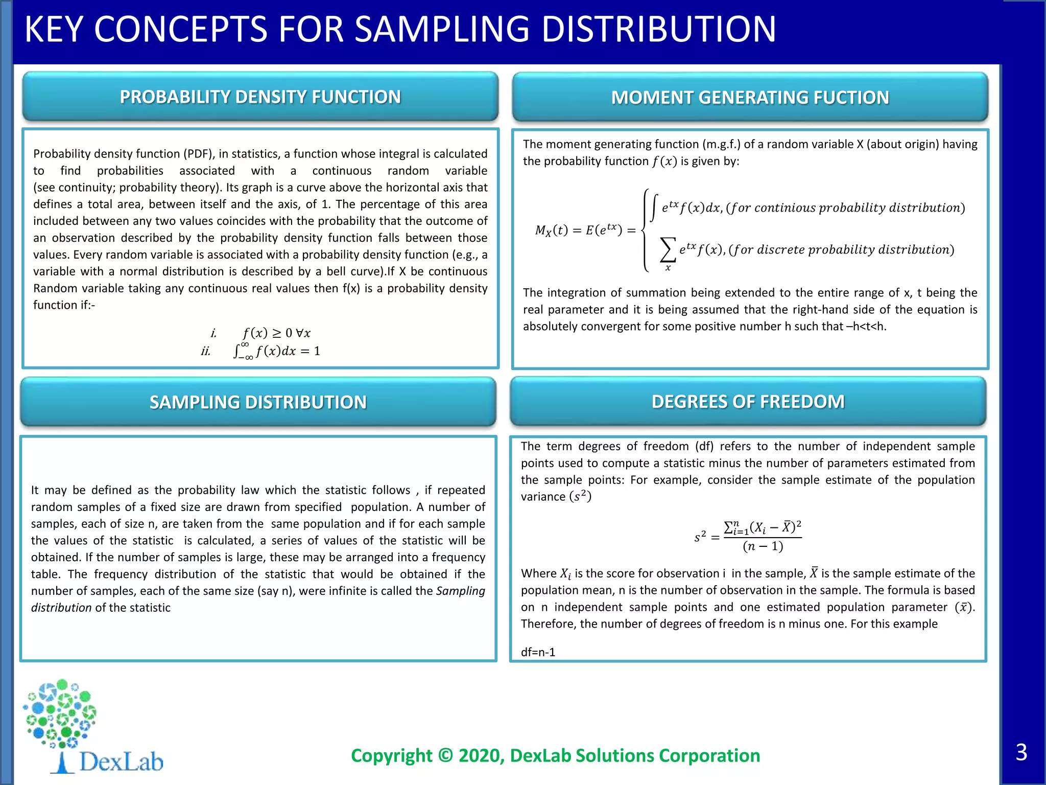
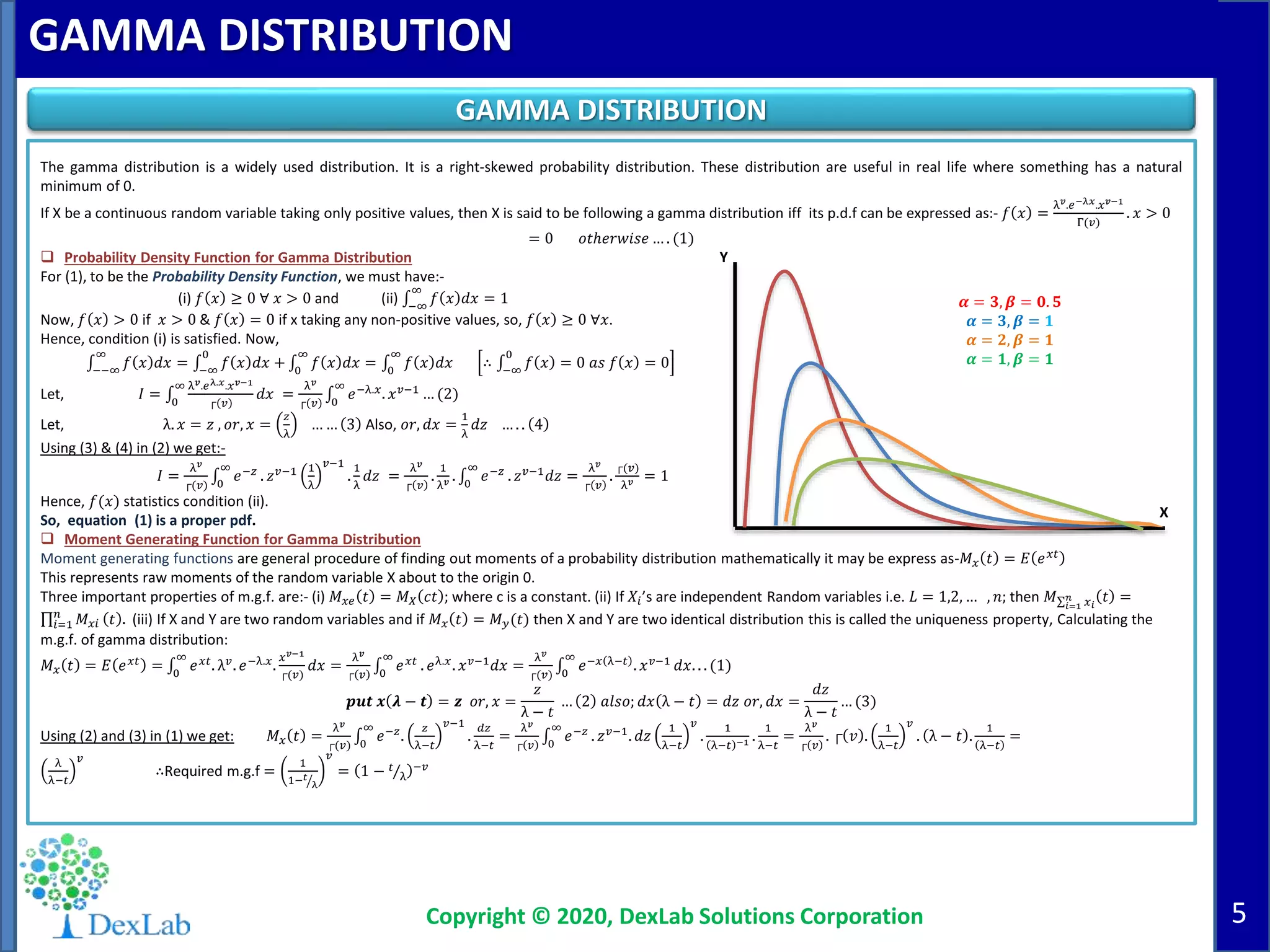
The document provides a comprehensive overview of statistical inference, covering topics such as probability density functions, moment generating functions, sampling distributions, and the gamma and beta distributions. It explains key concepts such as degrees of freedom, chi-square, and exponential distributions, with formulas for probability density functions and moment generating functions for each distribution. Additionally, it emphasizes the practical applications of these statistical concepts in various fields.


![Introduction-to-Probability-Distributions [Autosaved].pptx](https://cdn.slidesharecdn.com/ss_thumbnails/introduction-to-probability-distributionsautosaved-250401053355-25ab20ce-thumbnail.jpg?width=640&height=640&fit=bounds)


