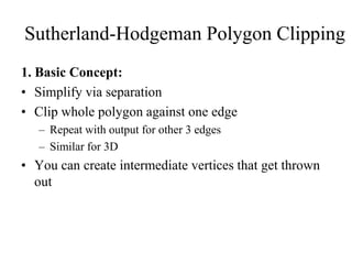
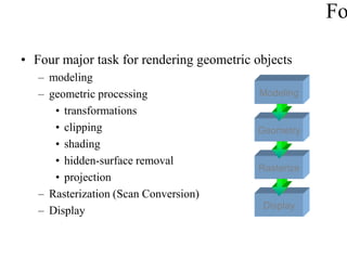
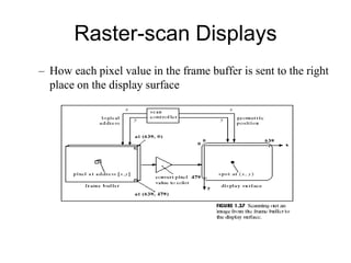
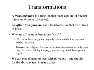
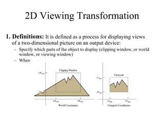
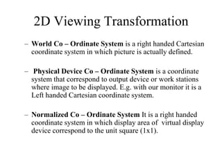
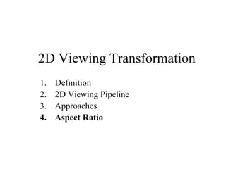
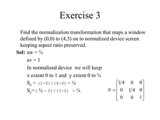
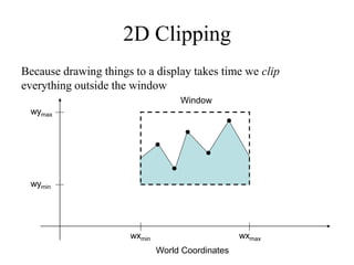
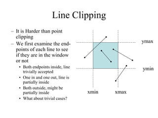
The document provides an overview of graphics systems and their components. It discusses four major tasks for rendering geometric objects: modeling, geometric processing, rasterization, and hidden surface removal. It also outlines the major sections which discuss input devices, hard-copy devices, video display devices, and graphics workstations.

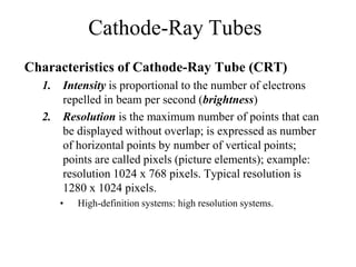
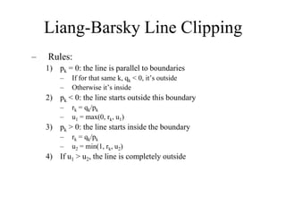
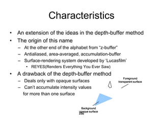
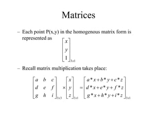
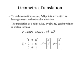
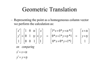
![Matrices
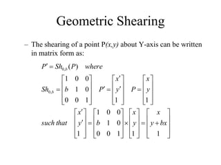
• Definition: A matrix is an n X m array of scalars, arranged
conceptually in n rows and m columns, where n and m are
positive integers. We use A, B, and C to denote matrices.
• If n = m, we say the matrix is a square matrix.
• We often refer to a matrix with the notation
A = [a(i,j)], where a(i,j) denotes the scalar in the ith row and
the jth column
• Note that the text uses the typical mathematical notation where
the i and j are subscripts. We'll use this alternative form as it is
easier to type and it is more familiar to computer scientists.](https://image.slidesharecdn.com/cgppts-mincompressed-230513065920-de3d2908/85/CGppts-min_compressed-pdf-81-320.jpg)
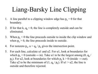
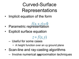
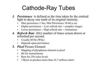
![Matrices
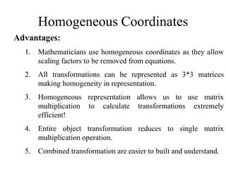
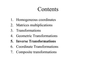
• Scalar-matrix multiplication:
A = [ a(i,j)]
• Matrix-matrix addition: A and B are both n X m
C = A + B = [a(i,j) + b(i,j)]
• Matrix-matrix multiplication: A is n X r and B is r X m
r
C = AB = [c(i,j)] where c(i,j) = a(i,k) b(k,j)
k=1](https://image.slidesharecdn.com/cgppts-mincompressed-230513065920-de3d2908/85/CGppts-min_compressed-pdf-82-320.jpg)
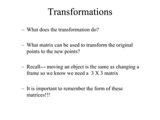

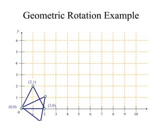
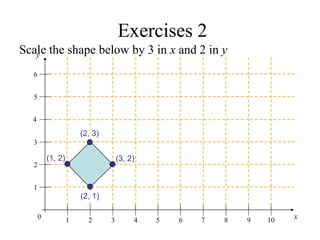
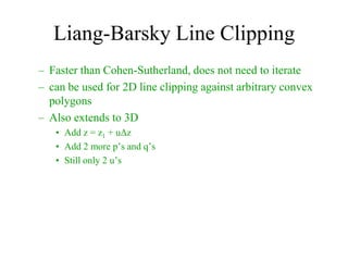
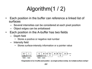
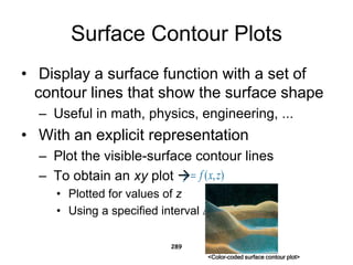
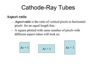
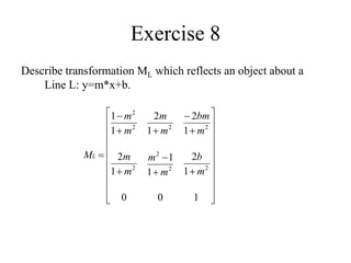
![Exercise 6
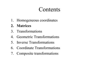
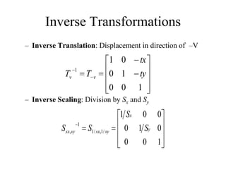
Rotate a triangle ABC A(0,0), B(1,1), C(5,2) by 450
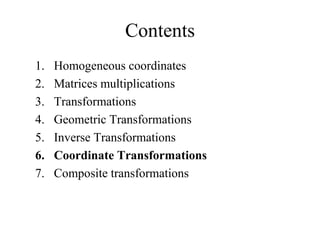
1. About origin (0,0)
2. About P(-1,-1)
1
0
0
0
2
2
2
2
0
2
2
2
2
45
R
1
0
0
1
2
2
2
2
2
1
2
2
2
2
)
1
,
1
(
,
45
R
1
1
1
2
1
0
5
1
0
]
[ABC](https://image.slidesharecdn.com/cgppts-mincompressed-230513065920-de3d2908/85/CGppts-min_compressed-pdf-137-320.jpg)
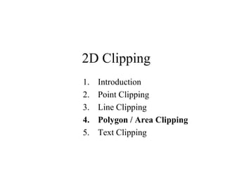
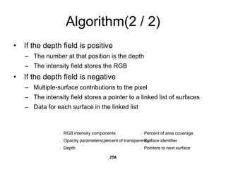
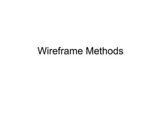
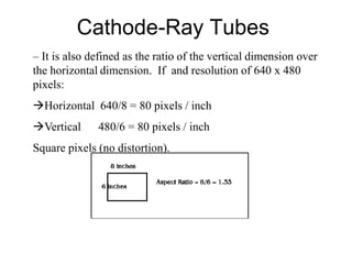
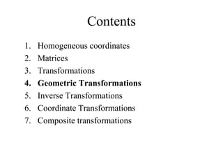
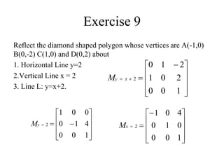
![Exercise 7
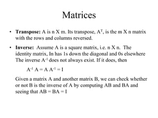
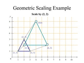
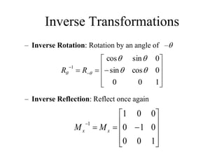
Magnify a triangle ABC A(0,0), B(1,1), C(5,2) twice keeping
point C(5,2) as fixed.
1
0
0
2
2
0
5
0
2
)
2
,
5
(
,
2
,
2
S
1
1
1
2
0
2
5
3
5
]
[ C
B
A
1
1
1
2
1
0
5
1
0
]
[ABC](https://image.slidesharecdn.com/cgppts-mincompressed-230513065920-de3d2908/85/CGppts-min_compressed-pdf-138-320.jpg)
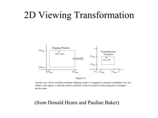

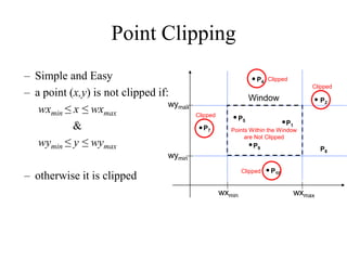
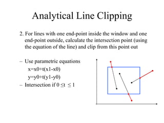
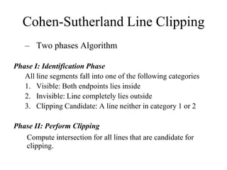
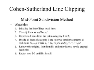
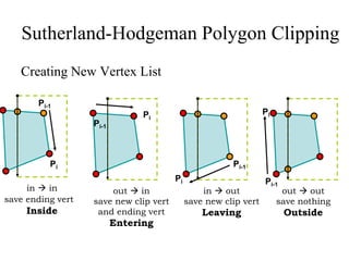
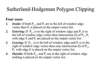
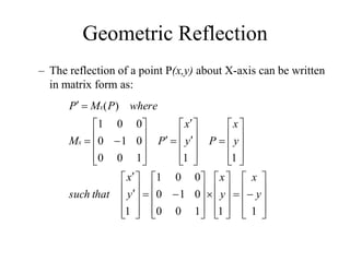
![Cohen-Sutherland Line Clipping
Every end-point is labelled with the appropriate region code
wymax
wymin
wxmin wxmax
Window
P3 [0001]
P6 [0000]
P5 [0000]
P7 [0001]
P10 [0100]
P9 [0000]
P4 [1000]
P8 [0010]
P12 [0010]
P11 [1010]
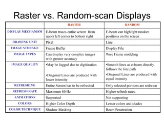
P13 [0101] P14 [0110]](https://image.slidesharecdn.com/cgppts-mincompressed-230513065920-de3d2908/85/CGppts-min_compressed-pdf-194-320.jpg)
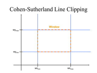
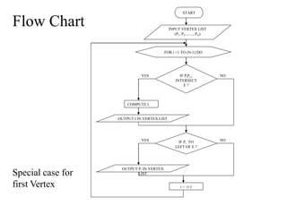
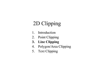
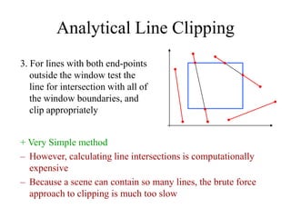
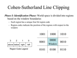
![Cohen-Sutherland Line Clipping
Visible Lines: Lines completely contained within the window
boundaries have region code [0000] for both end-points so are
not clipped
wymax
wymin
wxmin wxmax
Window
P3 [0001]
P6 [0000]
P5 [0000]
P7 [0001]
P10 [0100]
P9 [0000]
P4 [1000]
P8 [0010]
P12 [0010]
P11 [1010]
P13 [0101] P14 [0110]](https://image.slidesharecdn.com/cgppts-mincompressed-230513065920-de3d2908/85/CGppts-min_compressed-pdf-195-320.jpg)
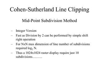
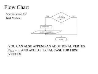
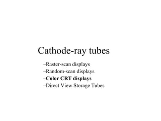
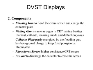
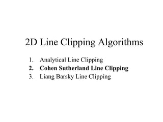
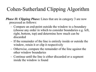
![Cohen-Sutherland Line Clipping
Invisible Lines: Any line with a common set bit in the region
codes of both end-points can be clipped completely
– The AND operation can efficiently check this
– Non Zero means Invisible
wymax
wymin
wxmin wxmax
Window
P3 [0001]
P6 [0000]
P5 [0000]
P7 [0001]
P10 [0100]
P9 [0000]
P4 [1000]
P8 [0010]
P12 [0010]
P11 [1010]
P13 [0101] P14 [0110]](https://image.slidesharecdn.com/cgppts-mincompressed-230513065920-de3d2908/85/CGppts-min_compressed-pdf-196-320.jpg)
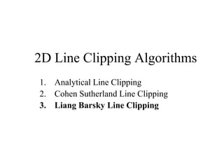
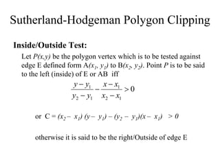
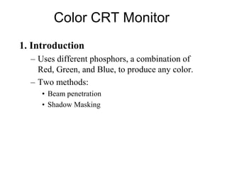
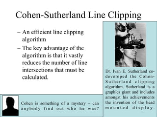
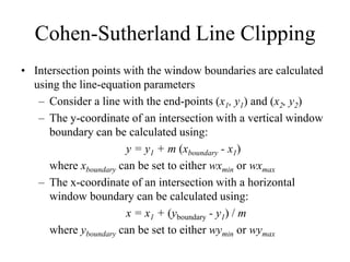
![Cohen-Sutherland Line Clipping
Clipping Candidates: Lines that cannot be identified as
completely inside or outside the window may or may not cross
the window interior. These lines are processed in Phase II.
– If AND operation result in 0 the line is candidate for clipping
wymax
wymin
wxmin wxmax
Window
P3 [0001]
P6 [0000]
P5 [0000]
P7 [0001]
P10 [0100]
P9 [0000]
P4 [1000]
P8 [0010]
P12 [0010]
P11 [1010]
P13 [0101] P14 [0110]](https://image.slidesharecdn.com/cgppts-mincompressed-230513065920-de3d2908/85/CGppts-min_compressed-pdf-197-320.jpg)
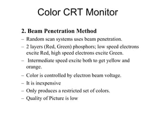
![Cohen-Sutherland Line Clipping
Example1: Consider the line P9 to P10 below
– Start at P10
– From the region codes
of the two end-points we
know the line doesn’t
cross the left or right
boundary
– Calculate the intersection
of the line with the bottom boundary
to generate point P10’
– The line P9 to P10’ is completely inside the window so is
retained
wymax
wymin
wxmin wxmax
Window
P10 [0100]
P9 [0000]
P10’ [0000]
P9 [0000]](https://image.slidesharecdn.com/cgppts-mincompressed-230513065920-de3d2908/85/CGppts-min_compressed-pdf-201-320.jpg)
![Cohen-Sutherland Line Clipping
Example 2: Consider the line P3 to P4 below
– Start at P4
– From the region codes
of the two end-points
we know the line
crosses the left
boundary so calculate
the intersection point to
generate P4’
– The line P3 to P4’ is completely outside the window so is
clipped
wymax
wymin
wxmin wxmax
Window
P4’ [1001]
P3 [0001]
P4 [1000]
P3 [0001]](https://image.slidesharecdn.com/cgppts-mincompressed-230513065920-de3d2908/85/CGppts-min_compressed-pdf-202-320.jpg)
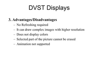
![Cohen-Sutherland Line Clipping
Example 3: Consider the line P7 to P8 below
– Start at P7
– From the two region
codes of the two
end-points we know
the line crosses the
left boundary so
calculate the
intersection point to
generate P7’
wymax
wymin
wxmin wxmax
Window
P7’ [0000]
P7 [0001] P8 [0010]
P8’ [0000]](https://image.slidesharecdn.com/cgppts-mincompressed-230513065920-de3d2908/85/CGppts-min_compressed-pdf-203-320.jpg)
![Cohen-Sutherland Line Clipping
Example 4: Consider the line P7’ to P8
– Start at P8
– Calculate the
intersection with the
right boundary to
generate P8’
– P7’ to P8’ is inside
the window so is
retained
wymax
wymin
wxmin wxmax
Window
P7’ [0000]
P7 [0001] P8 [0010]
P8’ [0000]](https://image.slidesharecdn.com/cgppts-mincompressed-230513065920-de3d2908/85/CGppts-min_compressed-pdf-204-320.jpg)