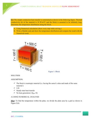
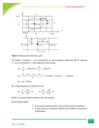
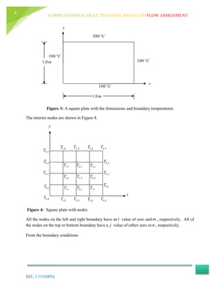
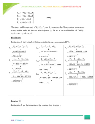
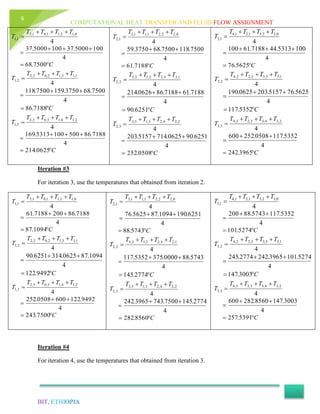
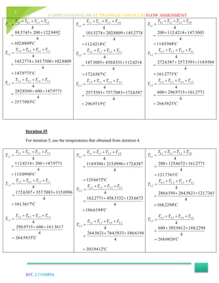
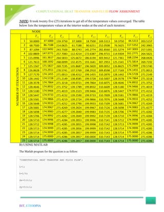
This document provides details of an assignment to determine the temperature distribution in a block using numerical analysis and MATLAB. It describes the block geometry, assumptions made, and steps taken to solve the problem using a numerical technique called the Gauss-Seidel method. The block is divided into a grid and the heat conduction equation is applied to each node to iteratively calculate the temperature at each point. The process is repeated over several iterations until the temperatures converge to a steady solution.

1. COMPUTATIONAL HEAT TRANSFER AND FLUID FLOW ASSIGNMENT
BIT, ETHIOPIA
1
BAHIRDAR UNIVERSITY
BAHIRDAR INSTITUTE OF TECHNOLOGY
FACULITY OF MECHANICAL AND INDUSTRIAL ENGINEERING
DEP’T (OF): MECHANICAL ENGINEERING
STREAM: THERMAL ENGINEERING
COMPUTATIONAL HEAT TRANSFER AND FLUID FLOW INDIVIDUAL
ASSIGNMENT
BY: LIJALEM TSIHAYE
ID.NO: 0800985
SECTION: D
SUBMITTED TO: MULUKEN .T (PhD Candi...)
Submission Date: 6/3/2012 E.C.

2. COMPUTATIONAL HEAT TRANSFER AND FLUID FLOW ASSIGNMENT
BIT, ETHIOPIA
2
Q1) The simple conduction heat transfer is constrained as shown in the following figure. Thermal
conductivity (k) of the material is 10 W/m*C and the block is assumed to be infinitely long.
Determine the temperature distribution along the block.
A. Using Numerical calculation (show every step while solving )
B. Write a Matlab code and show the temperature distribution and compare the result with the
Numerical result.
Figure 1: Block
SOLUTION
ASSUMPTION:
 The block is isentropic material (i.e. having the same k value and made of the same
material )
 2-D
 Steady state heat transfer
 No heat generation ( Qgen=0)
A.USING NUMERICAL ANALYSIS
Hint: To find the temperature within the plate, we divide the plate area by a grid as shown in
Figure 2(4).

3. COMPUTATIONAL HEAT TRANSFER AND FLUID FLOW ASSIGNMENT
BIT, ETHIOPIA
3
Figure 2: Plate area divided into a grid
The length L along the x axis is divided into m equal segments, while the width W along the
y axis is divided into n equal segments, hence giving
m
L
x  ……..Eqn (1)
n
W
y  ………Eqn (2)
5,4,3,2,1;4,3,2,1,
4
1,1,,1,1
, 



ji
TTTT
T
jijijiji
ji ………….Eqn (3)
myx 25.0
Re-writing Equations (1) and (2) we have
4
25.0
0.1



x
L
m
,
4
25.0
0.1



y
W
n
NOTE: Use Gauss-Seidel method to solve the problem
Gauss-Seidel method:
 Is an iterative method used to solve a linear system of equations.
 Is also known as Liebmann method or the method of successive
displacement.
tT
rT
x
y
),( ji ),1( ji 
)1,( ji
),1( ji 
)1,( ji
)0,0(
)0,(m
),0( n
bT
lT ),( ji
x
y
xy

4. COMPUTATIONAL HEAT TRANSFER AND FLUID FLOW ASSIGNMENT
BIT, ETHIOPIA
4
Figure 3: A square plate with the dimensions and boundary temperatures
The interior nodes are shown in Figure 4.
Figure 4: Square plate with nodes
All the nodes on the left and right boundary have ani value of zero and m , respectively. All of
the nodes on the top or bottom boundary have a j value of either zero or n , respectively.
From the boundary conditions
x
y
0,0T
0,1T 0,2T 0,3T 0,4T
1,0T
2,0T
3,0T
4,0T
1,1T 1,2T 1,3T 1,4T
2,1T 2,2T 2,3T
2,4T
3,1T 3,2T 3,3T
3,4T
4,1T 4,2T 4,3T 4,4T
C100
C100
C500
C100
m0.1
m0.1
x
y

5. COMPUTATIONAL HEAT TRANSFER AND FLUID FLOW ASSIGNMENT
BIT, ETHIOPIA
5











3,2,1,500
3,2,1,100
4,3,2,1,100
4,3,2,1,100
4,
0,
,4
,0
iT
iT
jT
jT
i
i
j
j
(***)
The corner nodal temperature of 0,44,44,0 ,, TTT and 0,0T are not needed. Now to get the temperature
at the interior nodes we have to write Equation (3) for all of the combinations of i and j ,
1,...,1;1,....,1  njmi .
Iteration #1
For iteration 1, start with all of the interior nodes having a temperature of C0 .
4
0,12,11,01,2
1,1
TTTT
T


4
10001000 

C 0000.50
4
1,13,12,02,2
2,1
TTTT
T


4
00.5001000 

C 5000.37
4
2,14,13,03,2
3,1
TTTT
T


4
5000.375001000 

C 3750.159
4
0,22,21,11,3
1,2
TTTT
T


4
10000000.500 

C 5000.37
4
1,23,22,12,3
2,2
TTTT
T


C


7500.18
4
5000.3705000.370
4
2,24,23,13,3
3,2
TTTT
T


4
7500.185003750.1590 

C 5313.169
4
0,32,31,21,4
1,3
TTTT
T


4
10005000.37100 

C 3750.59
4
1,33,32,22,4
2,3
TTTT
T


4
3750.5907500.18100 

C 5313.44
4
2,34,33,23,4
3,3
TTTT
T


4
5313.445005313.169100 

C 5157.203
Iteration #2
For iteration 2, use the temperatures that obtained from iteration 1.

6. COMPUTATIONAL HEAT TRANSFER AND FLUID FLOW ASSIGNMENT
BIT, ETHIOPIA
6
Iteration #3
For iteration 3, use the temperatures that obtained from iteration 2.
4
0,12,11,01,2
1,1
TTTT
T


4
7188.862007188.61 

C 1094.87
4
1,13,12,02,2
2,1
TTTT
T


C


9492.122
4
1094.870625.3146251.90
4
2,14,13,03,2
3,1
TTTT
T


4
9492.1226000508.252 

C 7500.243
4
0,22,21,11,3
1,2
TTTT
T


4
6251.1901094.875625.76 

C 5743.88
4
1,23,22,12,3
2,2
TTTT
T


C


2774.145
4
5743.880000.3755352.117
4
2,24,23,13,3
3,2
TTTT
T


4
2774.1457500.7433965.242 

C 8560.282
4
0,32,31,21,4
1,3
TTTT
T


4
5352.1175743.88200 

C 5274.101
4
1,33,32,22,4
2,3
TTTT
T


C


3003.147
4
5274.1013965.2422774.245
4
2,34,33,23,4
3,3
TTTT
T


4
3003.1478560.282600 

C 5391.257
Iteration #4
For iteration 4, use the temperatures that obtained from iteration 3.
4
0,12,11,01,2
1,1
TTTT
T


4
1005000.371005000.37 

C 7500.68
4
1,13,12,02,2
2,1
TTTT
T


C


7188.86
4
7500.683750.1597500.118
4
2,14,13,03,2
3,1
TTTT
T


4
7188.865001005313.169 

C 0625.214
4
0,22,21,11,3
1,2
TTTT
T


4
7500.1187500.683750.59 

C 7188.61
4
1,23,22,12,3
2,2
TTTT
T


C


6251.90
4
7188.617188.860626.214
4
2,24,23,13,3
3,2
TTTT
T


4
6251.900625.7145157.203 

C 0508.252
4
0,32,31,21,4
1,3
TTTT
T


4
1005313.447188.61100 

C 5625.76
4
1,33,32,22,4
2,3
TTTT
T


C


5352.117
4
5625.765157.2030625.190
4
2,34,33,23,4
3,3
TTTT
T


4
5352.1170508.252600 

C 3965.242

7. COMPUTATIONAL HEAT TRANSFER AND FLUID FLOW ASSIGNMENT
BIT, ETHIOPIA
7
Iteration #5
For iteration 5, use the temperatures that obtained from iteration 4.
4
0,12,11,01,2
1,1
TTTT
T


4
9492.1222005743.88 

C 8809.102
4
1,13,12,02,2
2,1
TTTT
T


C


9771.147
4
8809.1027500.3432774.145
4
2,14,13,03,2
3,1
TTTT
T


4
9771.1476008560.282 

C 7083.257
4
0,22,21,11,3
1,2
TTTT
T


4
2774.1458809.2025274.101 

C 4214.112
4
1,23,22,12,3
2,2
TTTT
T


C


6387.172
4
4214.1128331.4303003.147
4
2,24,23,13,3
3,2
TTTT
T


4
6387.1727083.7575391.257 

C 9715.296
4
0,32,31,21,4
1,3
TTTT
T


4
3003.1474214.112200 

C 9304.114
4
1,33,32,22,4
2,3
TTTT
T


C


2771.161
4
9304.1145391.2576387.272
4
2,34,33,23,4
3,3
TTTT
T


4
2771.1619715.296600 

C 5621.264
4
0,12,11,01,2
1,1
TTTT
T


4
9771.1472004214.112 

C 0996.115
4
1,13,12,02,2
2,1
TTTT
T


C


3617.161
4
0996.1157083.3576387.172
4
2,14,13,03,2
3,1
TTTT
T


4
3617.1616009715.296 

C 5833.264
4
0,22,21,11,3
1,2
TTTT
T


4
6387.1720996.2159304.114 

C 6672.125
4
1,23,22,12,3
2,2
TTTT
T


C


6194.186
4
6672.1253332.4582771.162
4
2,24,23,13,3
3,2
TTTT
T


4
6194.1865833.7645621.264 

C 9412.303
4
0,32,31,21,4
1,3
TTTT
T


4
2771.1616672.125200 

C 7361.121
4
1,33,32,22,4
2,3
TTTT
T


C


2294.168
4
7361.1215621.2646194.286
4
2,34,33,23,4
3,3
TTTT
T


4
2294.1689412.303600 

C 0426.268

8. COMPUTATIONAL HEAT TRANSFER AND FLUID FLOW ASSIGNMENT
BIT, ETHIOPIA
8
NOTE: It took twenty five (25) iterations to get all of the temperature values converged. The table
below lists the temperature values at the interior nodes at the end of each iteration:
B) USING MATLAB
The Matlab program for the question is as follow:
‘COMPUTATIOAL HEAT TRANSFER AND FLUID FLOW’;
L=1;
h=L/4;
dx=0:h:L;
dy=0:h:L;
NODE
NUMBEROFITERATIONS
1,1T 2,1T 3,1T 1,2T 2,2T 3,2T 1,3T 2,3T 3,3T
1 50.0000 37.5000 159.3750 37.5000 18.7500 169.5313 59.3750 44.5313 203.5157
2 68.7500 86.7188 214.0625 61.7188 90.6251 252.0508 76.5625 117.5352 242.3965
3 87.1094 122.9492 243.7500 88.5743 145.2774 282.8560 101.5274 147.3003 257.5391
4 102.8809 147.9771 257.7083 112.4214 172.6387 296.9715 114.9304 161.2771 264.5621
5 115.0996 161.3617 264.5833 125.6672 186.6194 303.9412 121.7361 168.2294 268.0426
6 121.7613 168.1692 268.0099 132.4575 193.1641 307.2953 125.1541 171.5814 269.7192
7 125.1567 171.5827 269.7195 135.8687 196.5820 309.0052 126.8625 173.2909 270.5740
8 126.8628 173.2911 270.5741 137.5769 198.2910 309.8598 127.7169 174.1455 271.0013
9 127.7170 174.1455 271.0013 138.4312 199.1455 310.2870 128.1442 174.5728 271.2149
10 128.1442 174.5728 271.2149 138.8585 199.5728 310.5007 128.3578 174.7864 271.3218
11 128.3578 174.7864 271.3218 139.0721 199.7864 310.6075 128.4646 174.8932 271.3752
12 128.4646 174.8932 271.3752 139.1789 199.8932 310.6609 128.5180 174.9466 271.4019
13 128.5180 174.9466 271.4019 139.2323 199.9466 310.6876 128.5447 174.9733 271.4152
14 128.5447 174.9733 271.4152 139.2590 199.9733 310.7009 128.5581 174.9866 271.4219
15 128.5581 174.9866 271.4219 139.2724 199.9866 310.7076 128.5648 174.9933 271.4252
16 128.5648 174.9933 271.4252 139.2790 199.9933 310.7109 128.5681 174.9967 271.4269
17 128.5681 174.9967 271.4269 139.2824 199.9967 310.7126 128.5698 174.9983 271.4277
18 128.5698 174.9983 271.4277 139.2840 199.9983 310.7135 128.5706 174.9992 271.4282
19 128.5706 174.9992 271.4282 139.2849 199.9992 310.7139 128.5710 174.9996 271.4284
20 128.5710 174.9996 271.4284 139.2853 199.9996 310.7141 128.5712 174.9998 271.4285
21 128.5712 174.9998 271.4285 139.2855 199.9998 310.7142 128.5713 174.9999 271.4285
22 128.5713 174.9999 271.4285 139.2856 199.9999 310.7142 128.5714 174.9999 271.4285
23 128.5714 174.9999 271.4285 139.2857 199.9999 310.7143 128.5714 175.0000 271.4286
24 128.5714 175.0000 271.4286 139.2857 200.0000 310.7143 128.5714 175.0000 271.4286
25 128.5714 175.0000 271.4286 139.2857 200.0000 310.7143 128.5714 175.0000 271.4286

9. COMPUTATIONAL HEAT TRANSFER AND FLUID FLOW ASSIGNMENT
BIT, ETHIOPIA
9
T=zeros(length(dx),length(dy));
T(:,1)=100;
T(:,end)=100;
T(end,:)=100;
T(1,:)=500;
for k=1:25;
for i=2:length(dx)-1;
for j=2:length(dy)-1;
T(i,j)=0.25*[T(i-1,j)+T(i+1,j)+T(i,j-1)+T(i,j+1)];
end
end
end
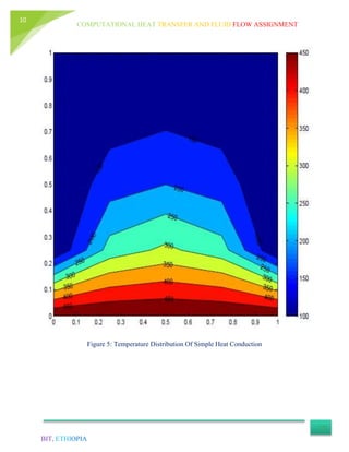
contourf(dx,dy,T,'ShowText','on')
colormap jet
T
T =
500.0000 500.0000 500.0000 500.0000 500.0000
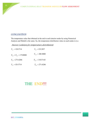
100.0000 271.4286 310.7143 271.4286 100.0000
100.0000 175.0000 200.0000 175.0000 100.0000
100.0000 128.5714 139.2857 128.5714 100.0000
100.0000 100.0000 100.0000 100.0000 100.0000

10. COMPUTATIONAL HEAT TRANSFER AND FLUID FLOW ASSIGNMENT
BIT, ETHIOPIA
10
Figure 5: Temperature Distribution Of Simple Heat Conduction

11. COMPUTATIONAL HEAT TRANSFER AND FLUID FLOW ASSIGNMENT
BIT, ETHIOPIA
11
CONCLUSTION
The temperature value that obtained at the end in each interior nodes by using Numerical
Analysis and Matlab is the same. So, the temperature distribution value on each nodes is (i.e.
Answer (solution for temperature distribution)
128.57141,1 T 2857.1391,2 T
0000.1752,32,1  TT
0000.2002,2 T
4286.2713,1 T 7143.3103,2 T
4286.2713,3 T
THE END!!!
5714.1281,3 T

12. COMPUTATIONAL HEAT TRANSFER AND FLUID FLOW ASSIGNMENT
BIT, ETHIOPIA
12