Downloaded 257 times
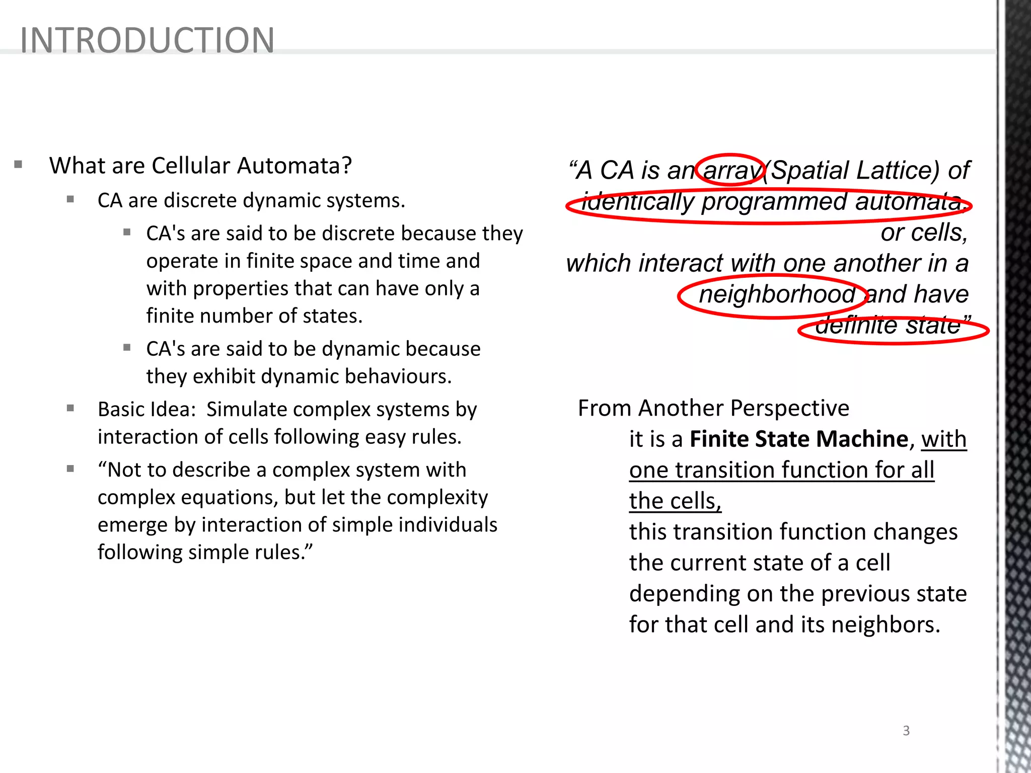
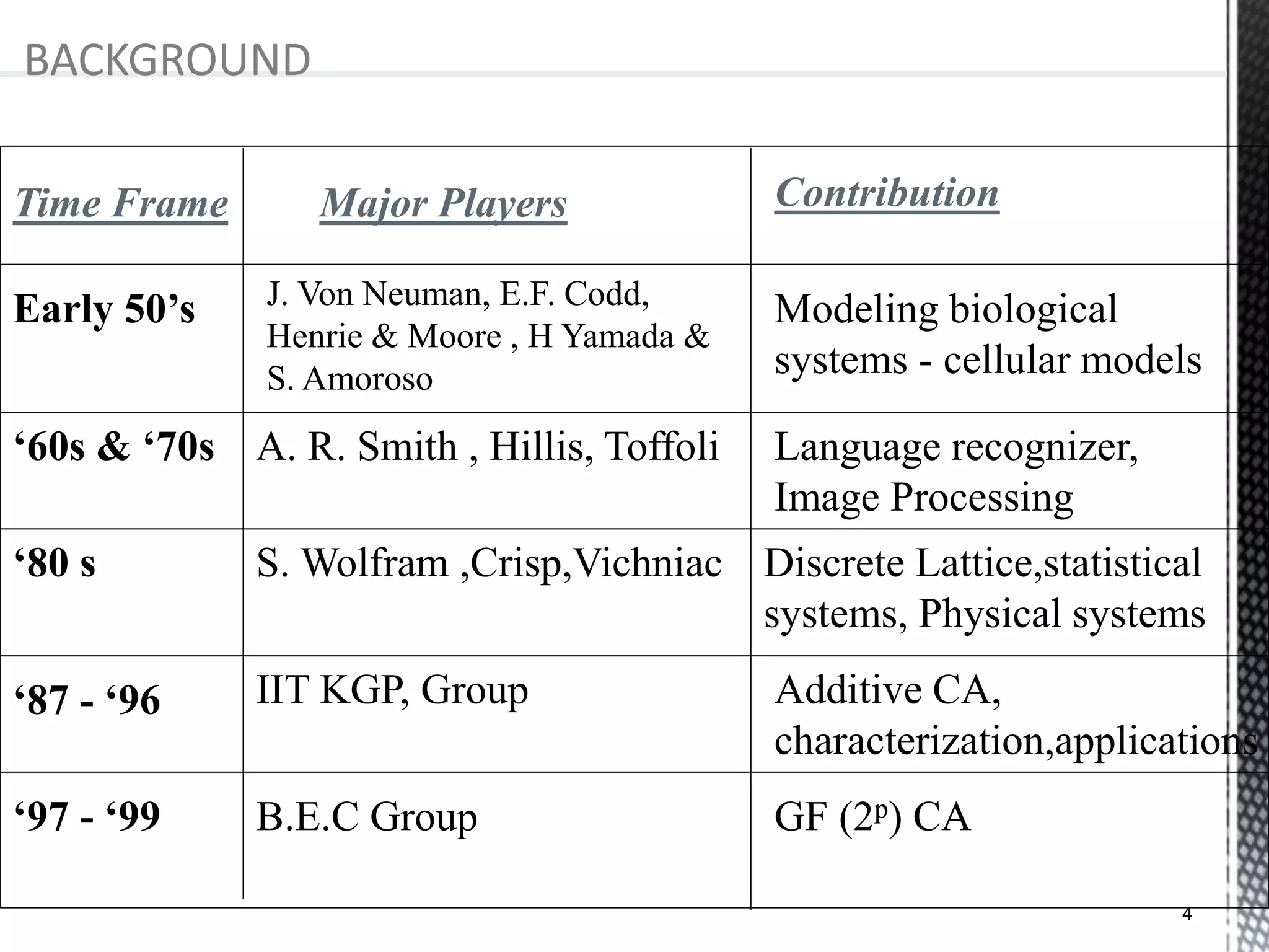
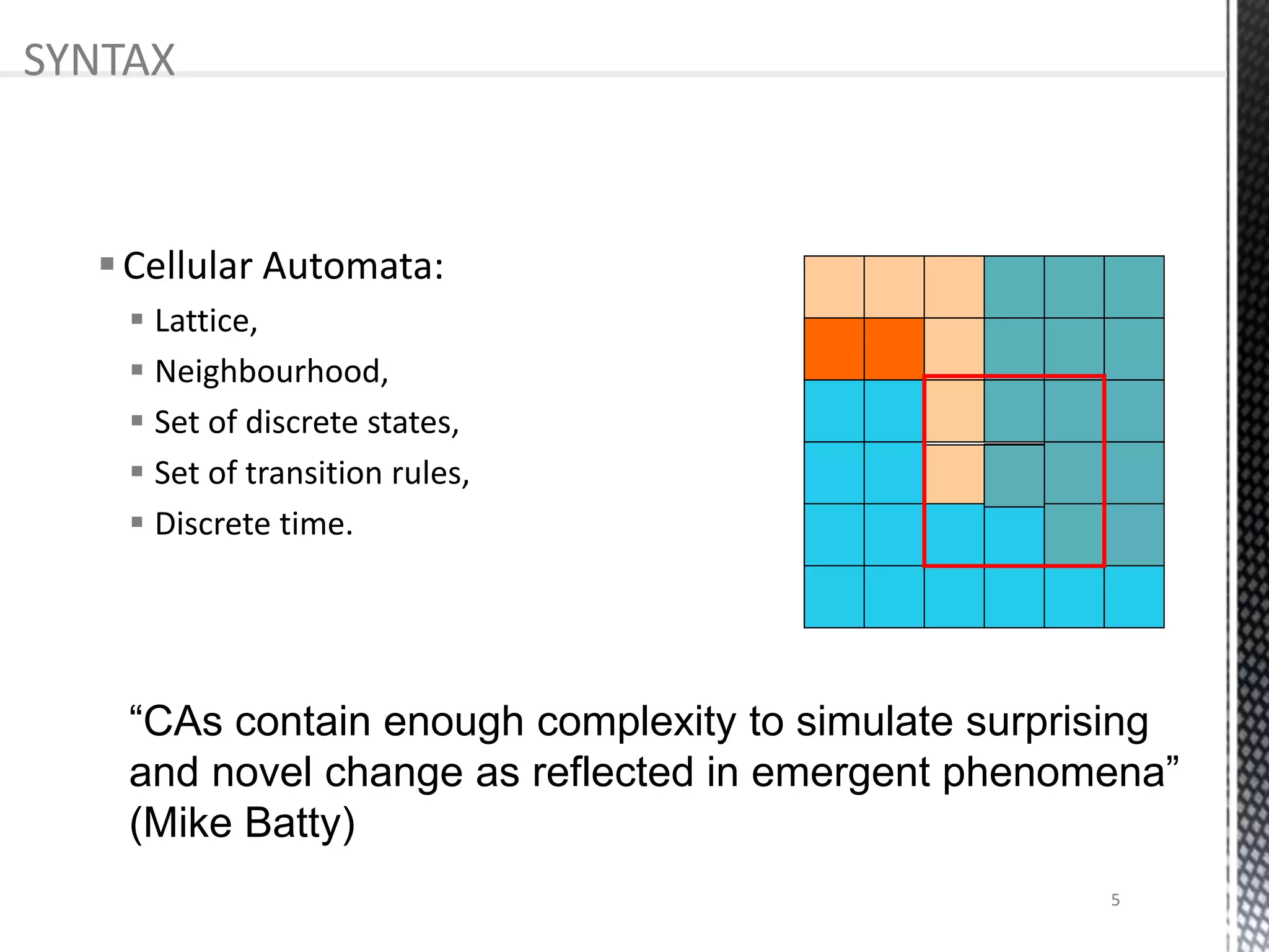
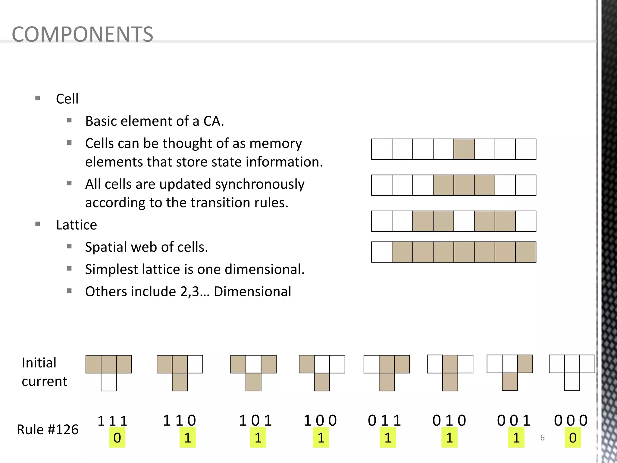
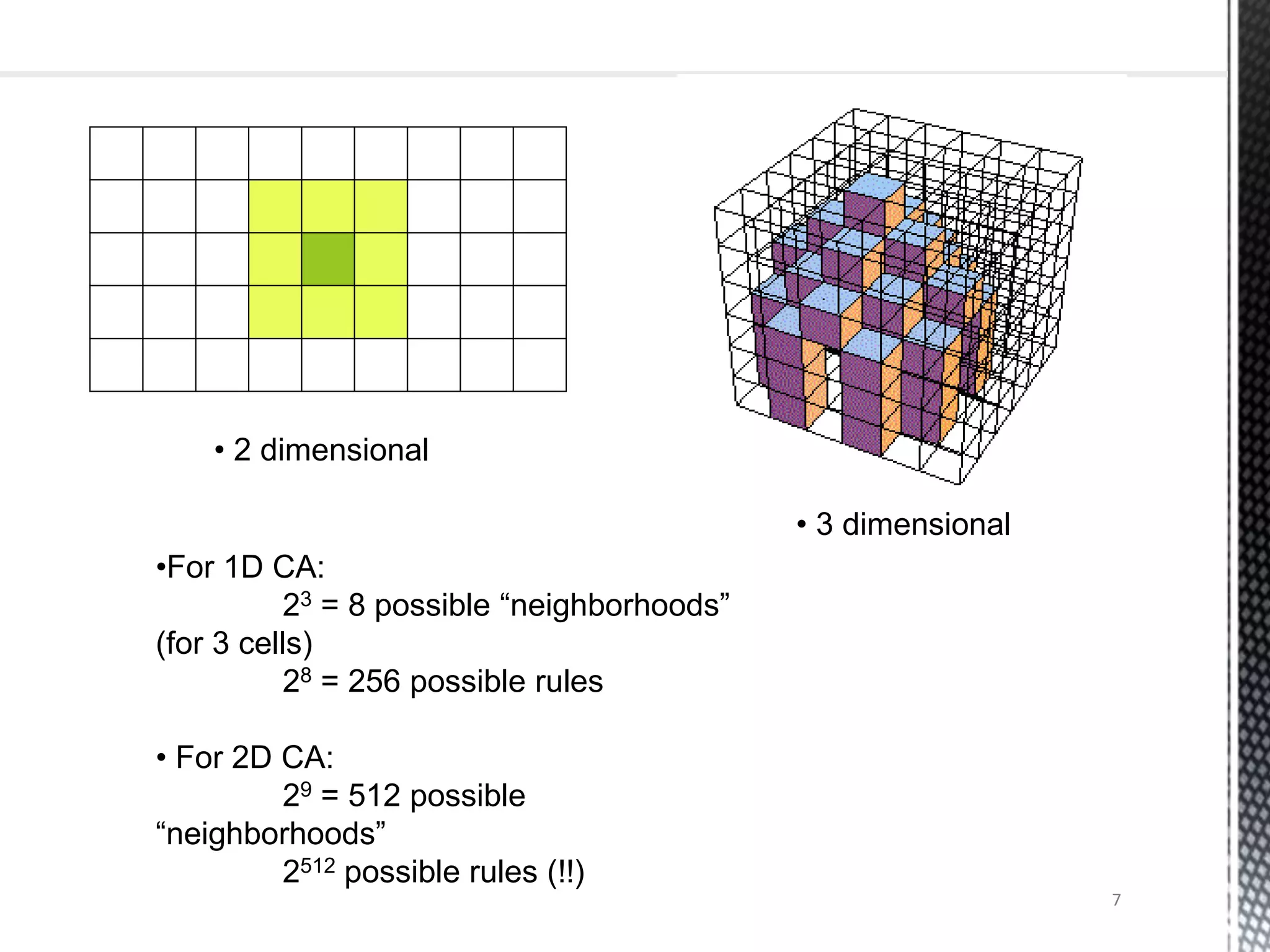
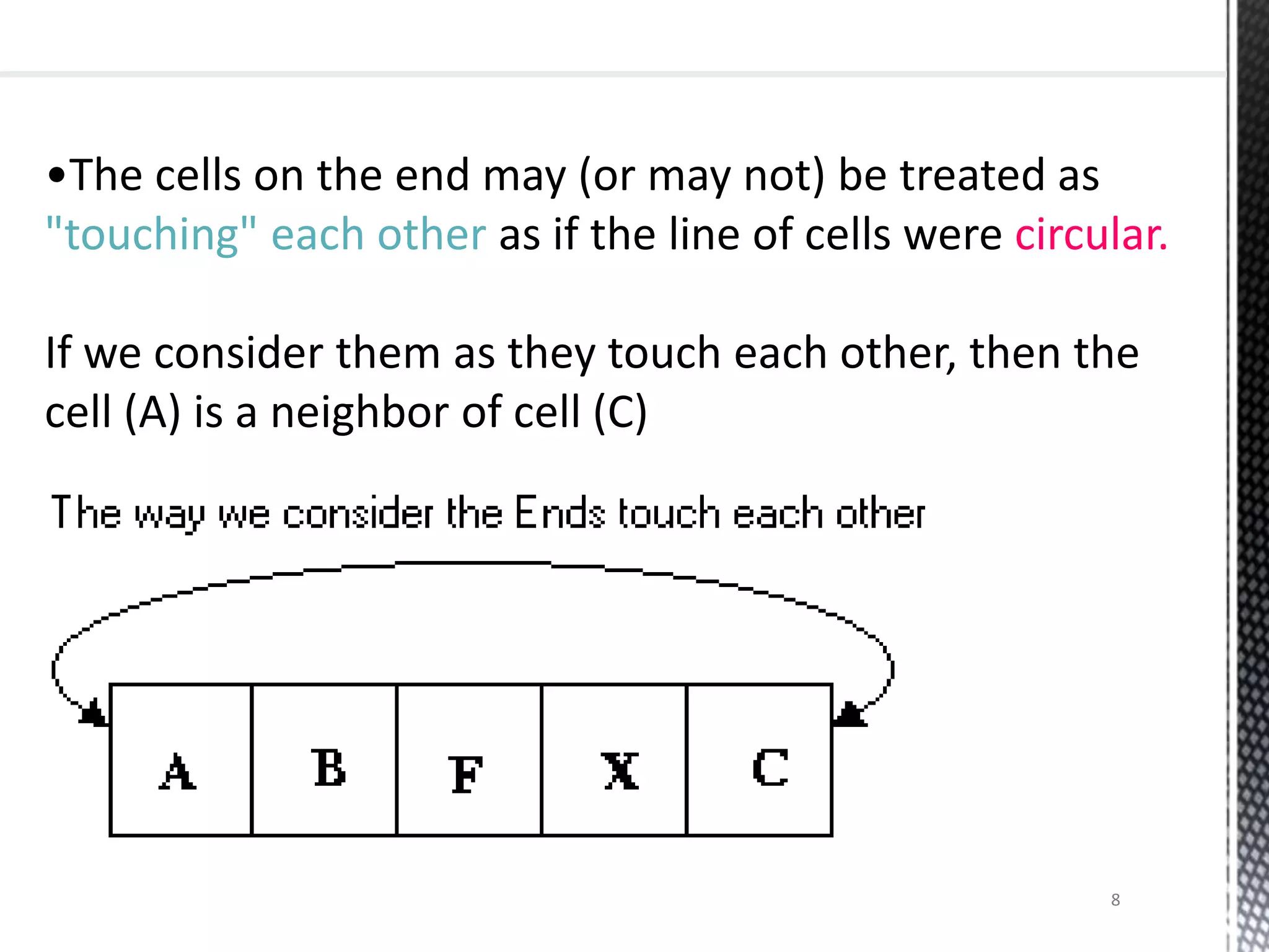
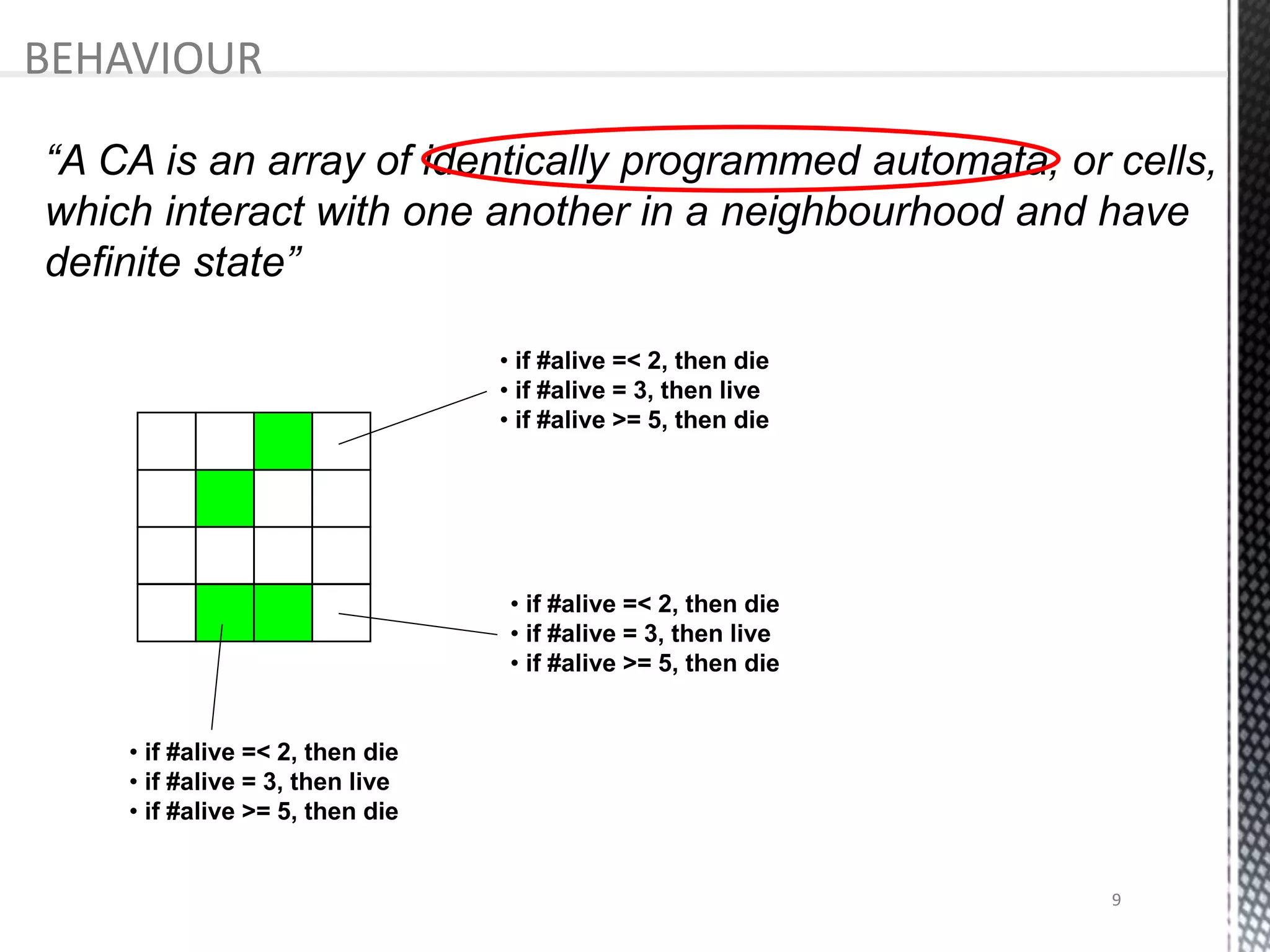
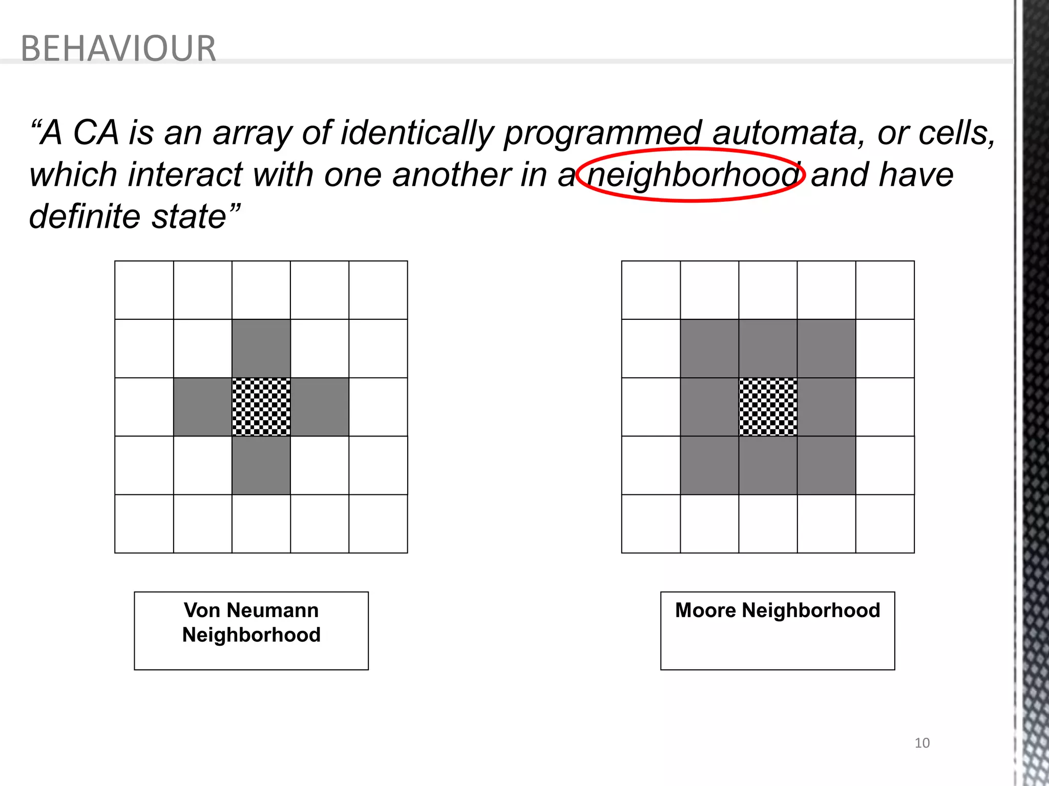
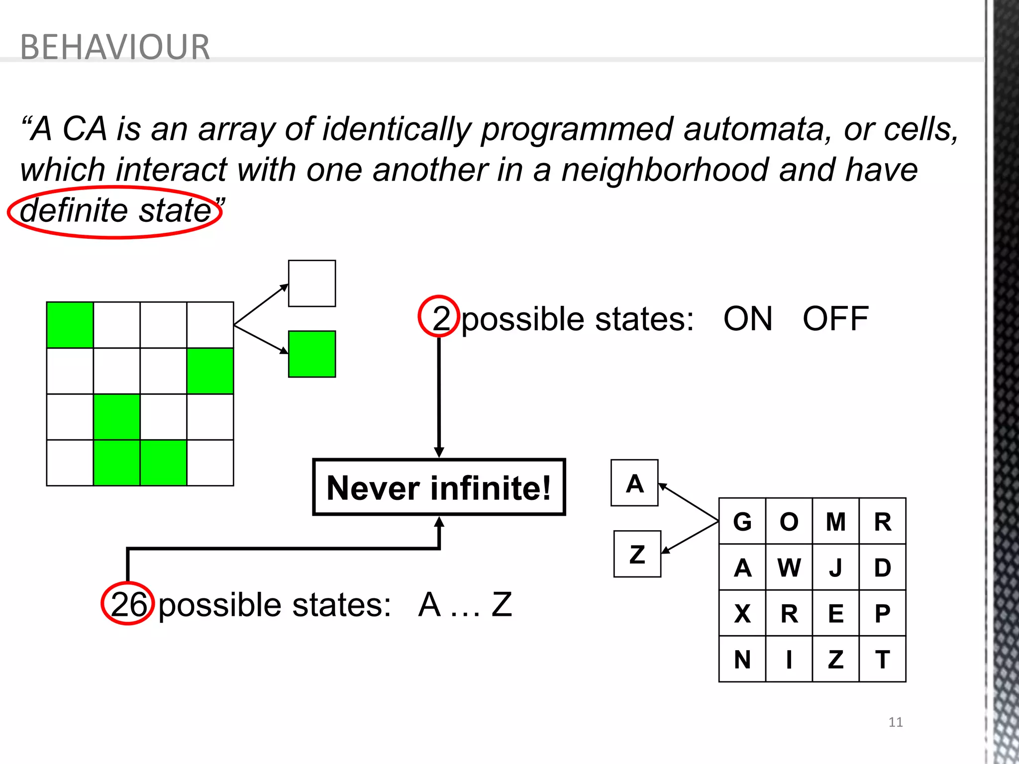
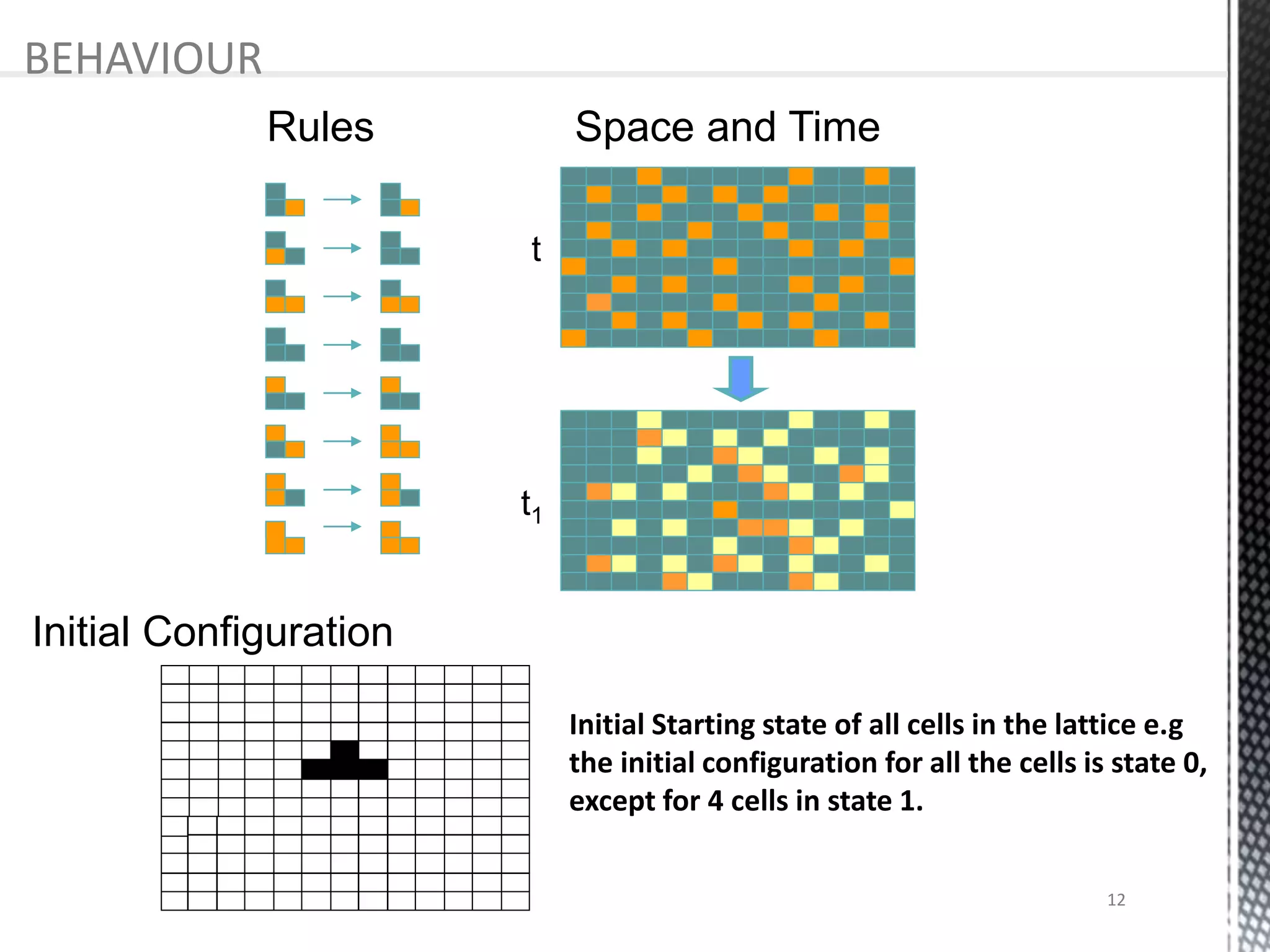
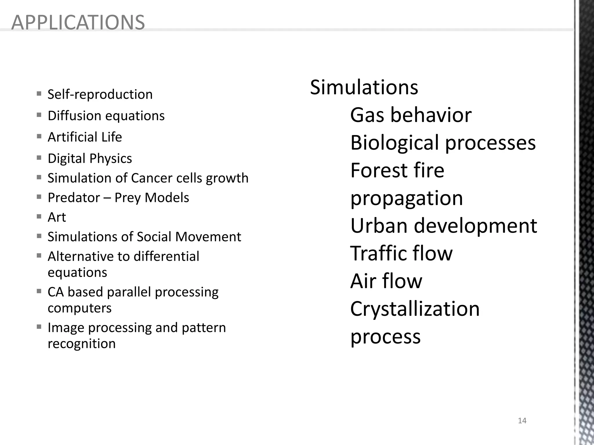
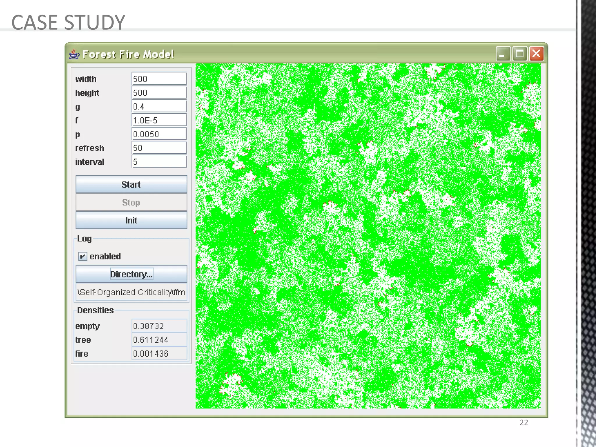
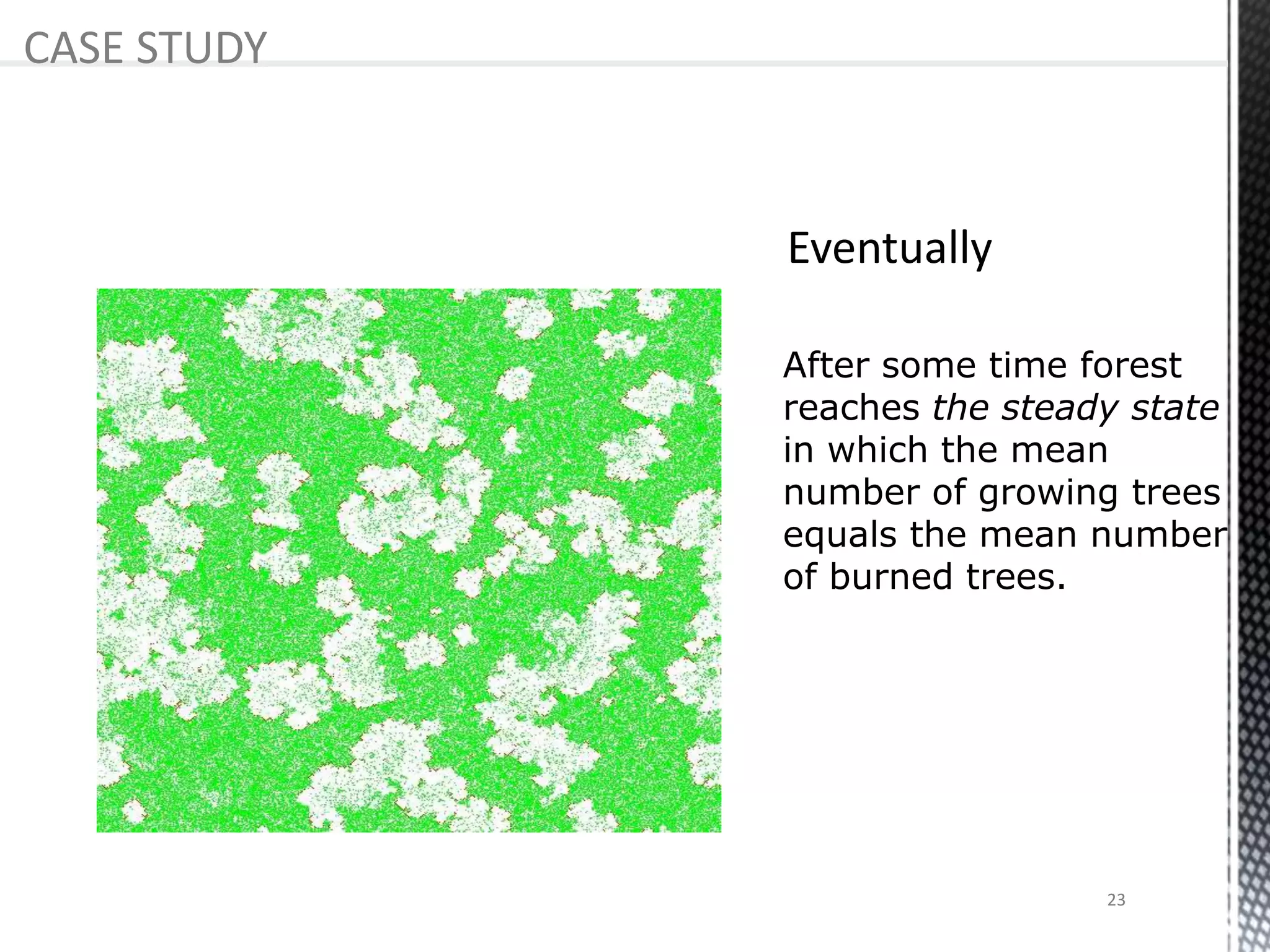
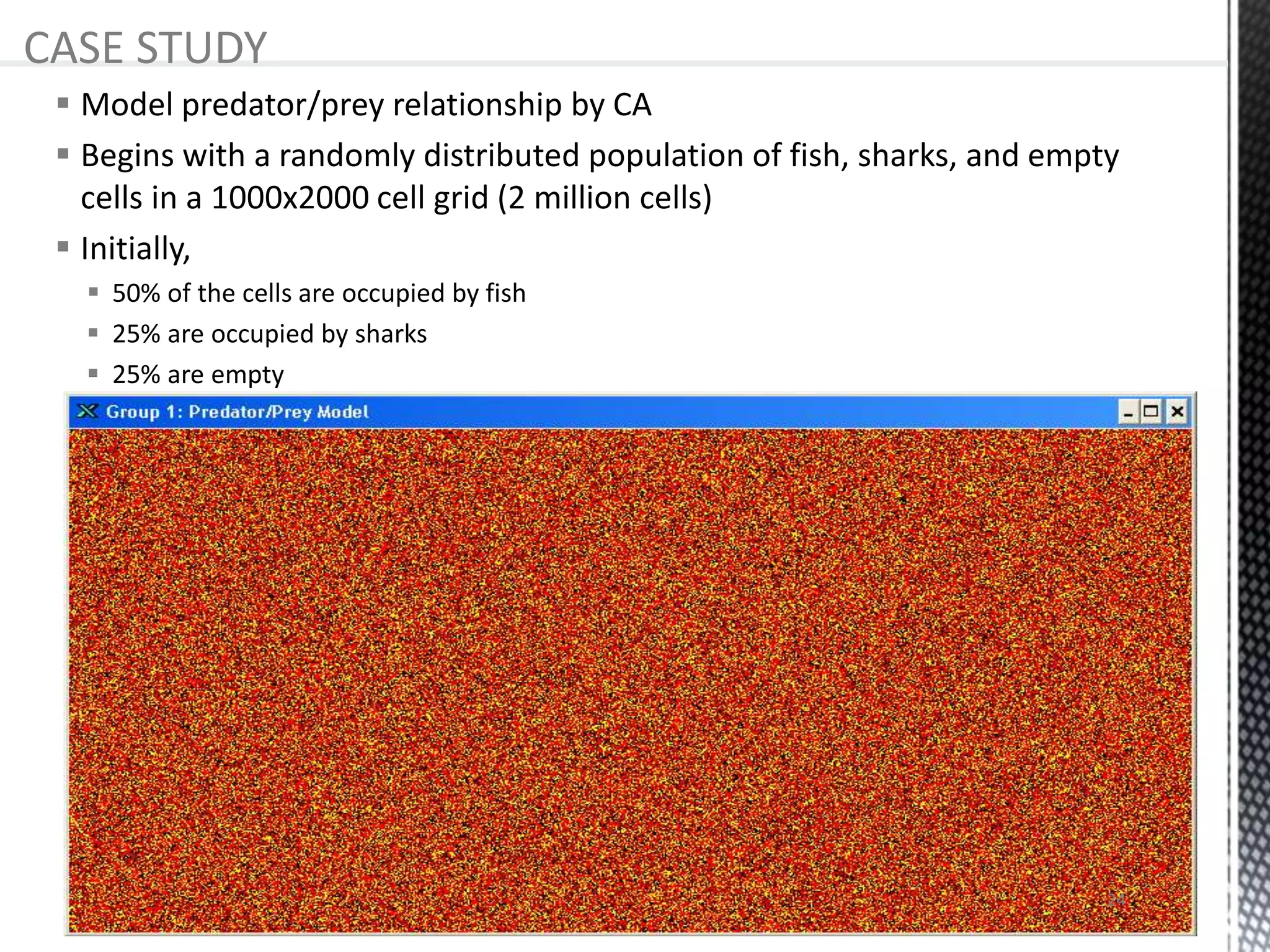
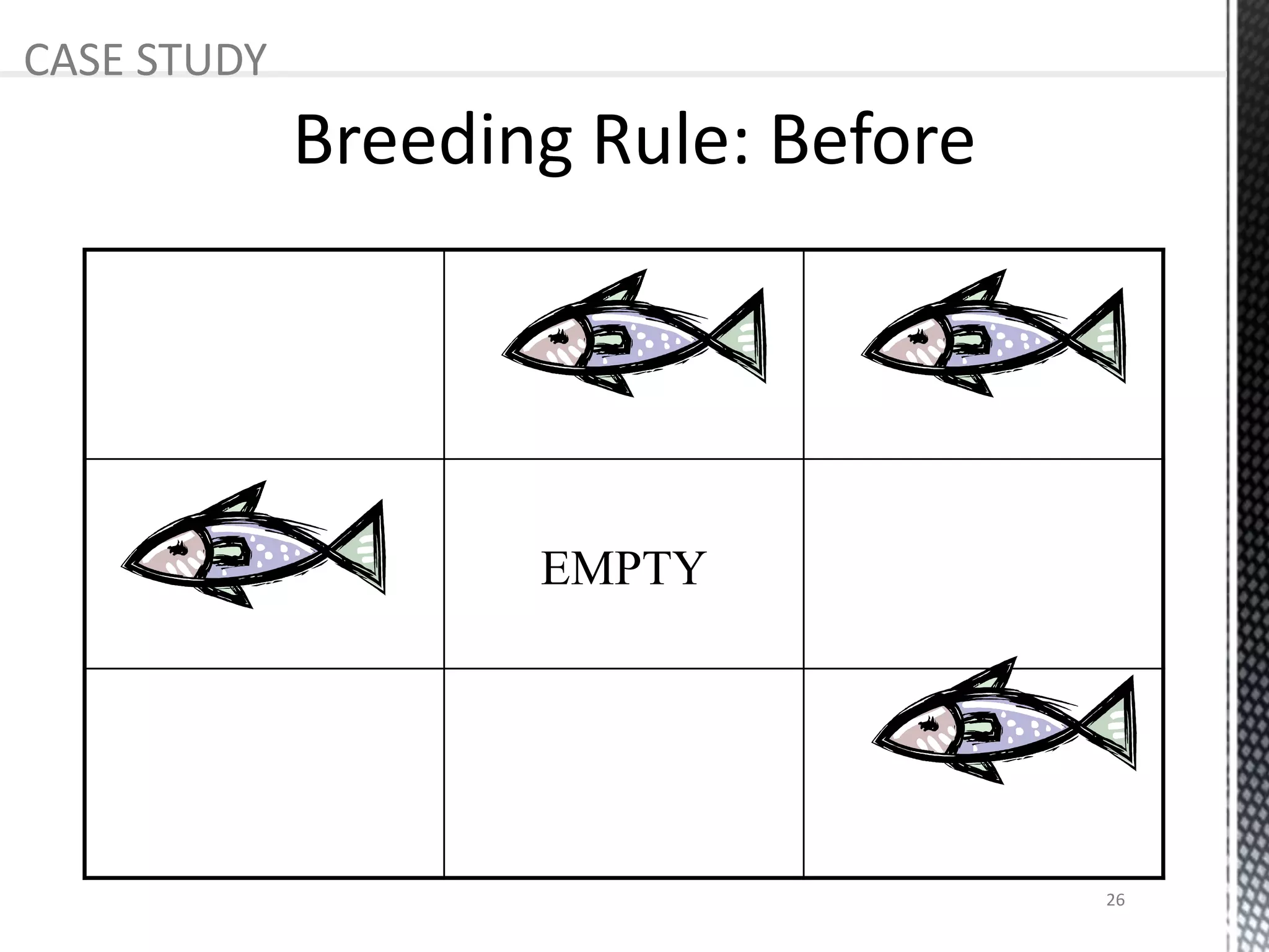
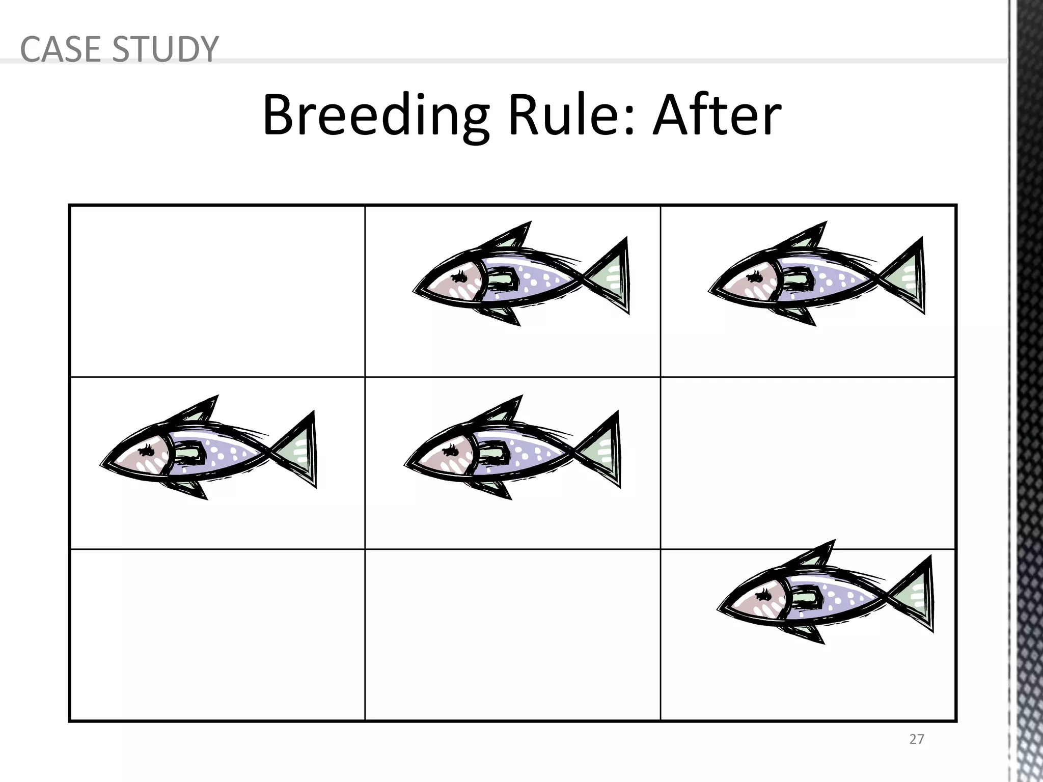
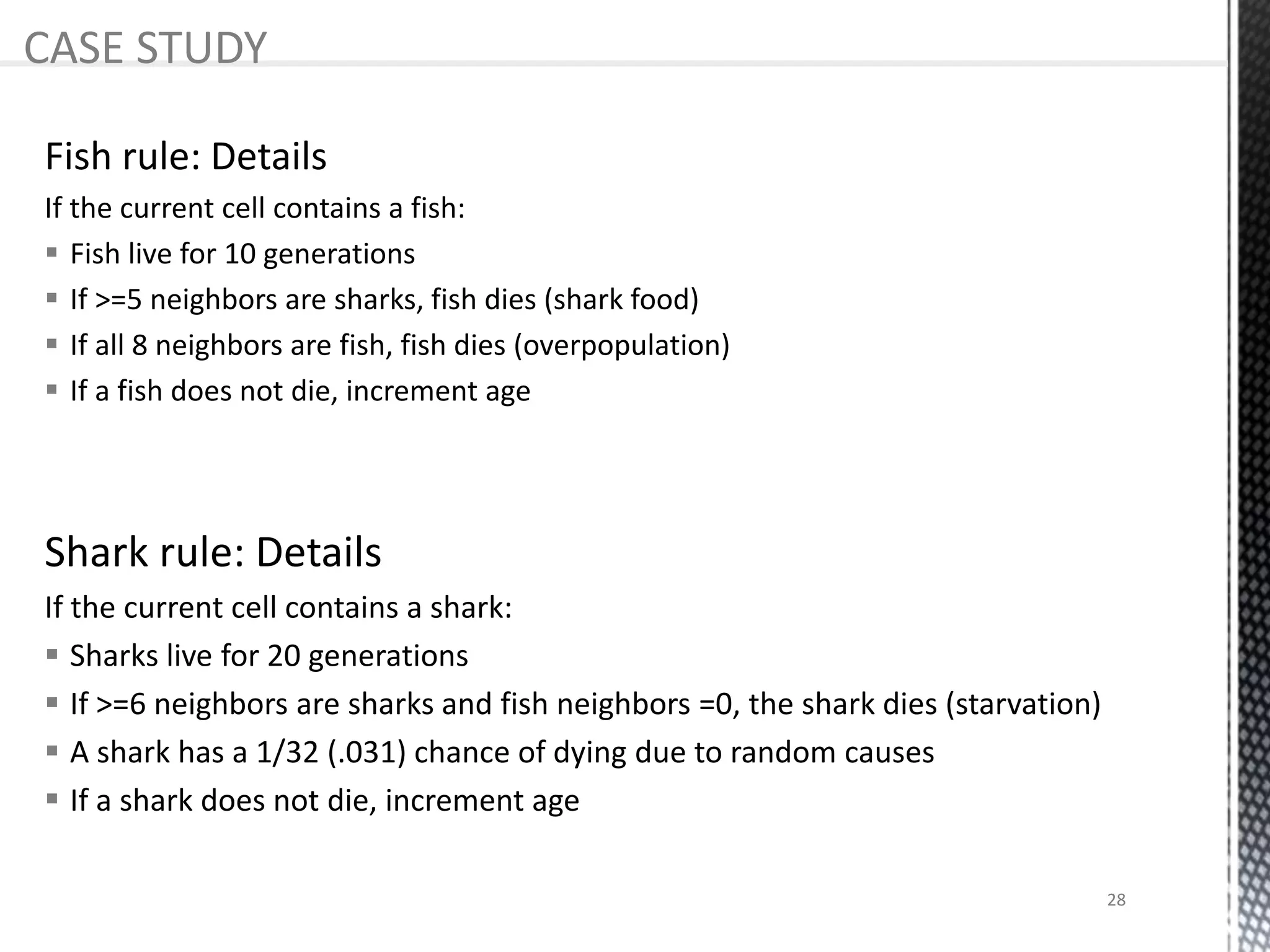
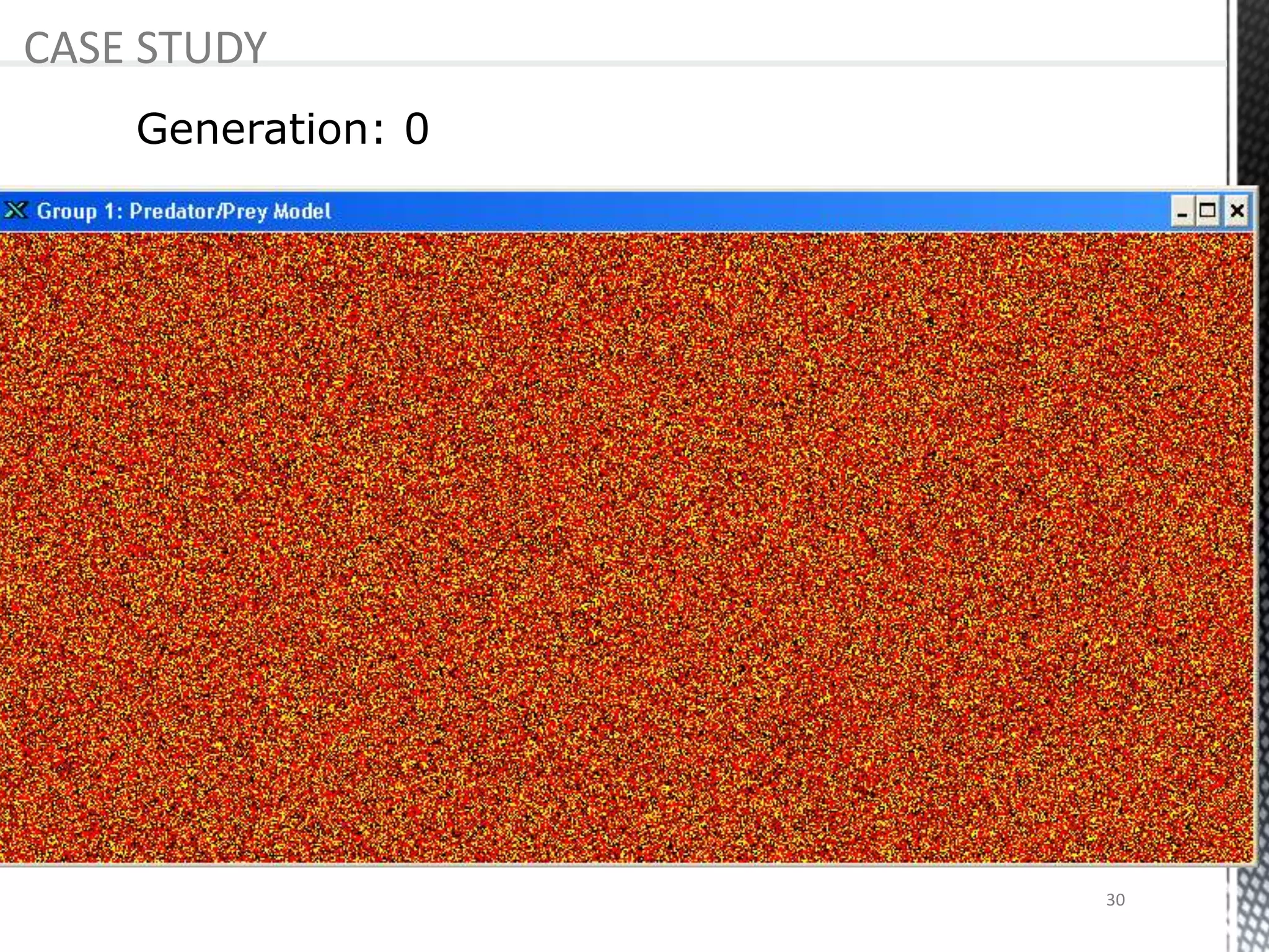
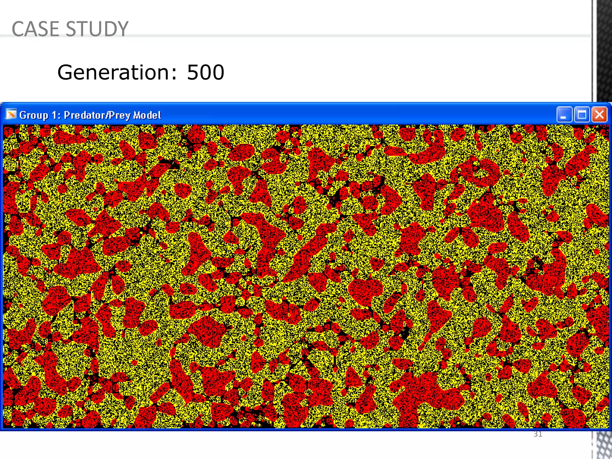
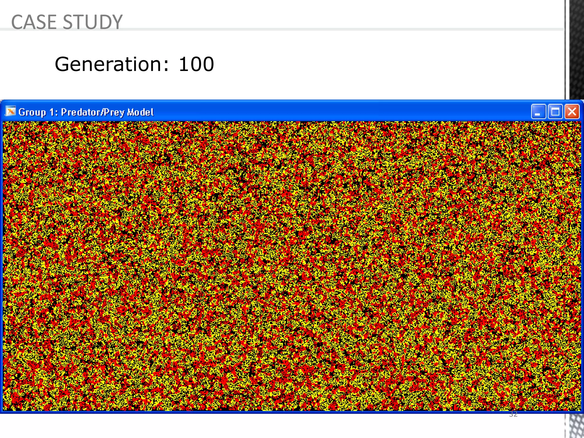
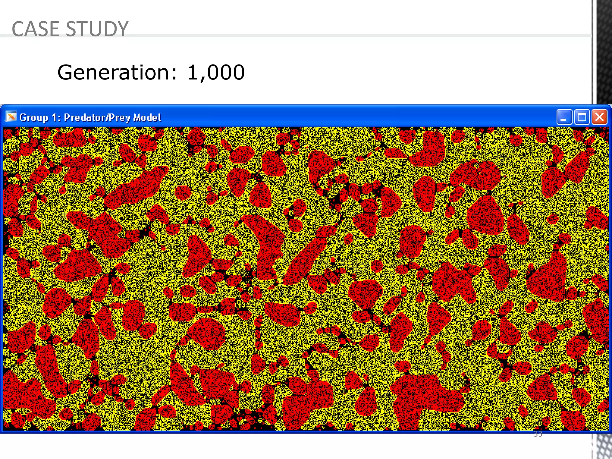
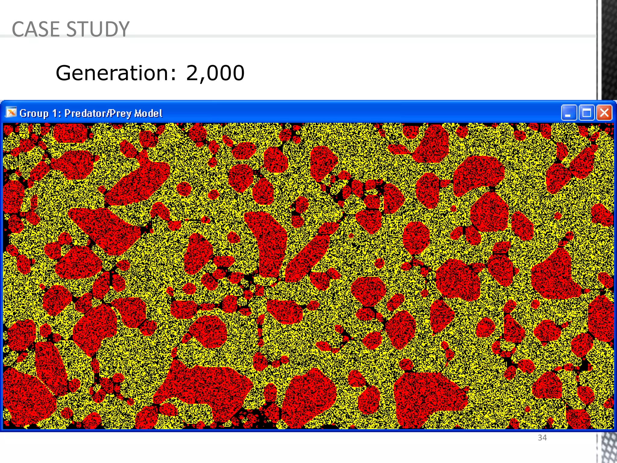
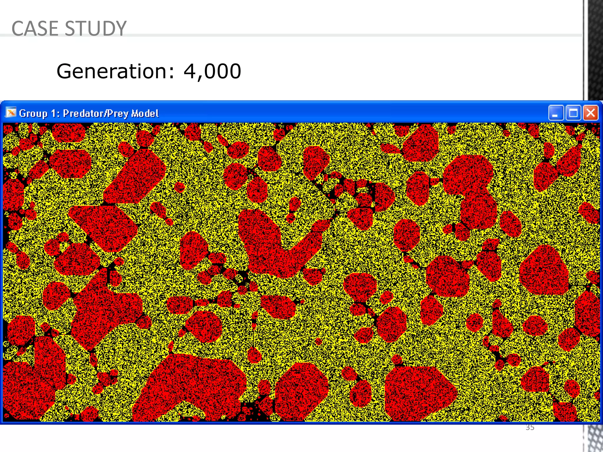
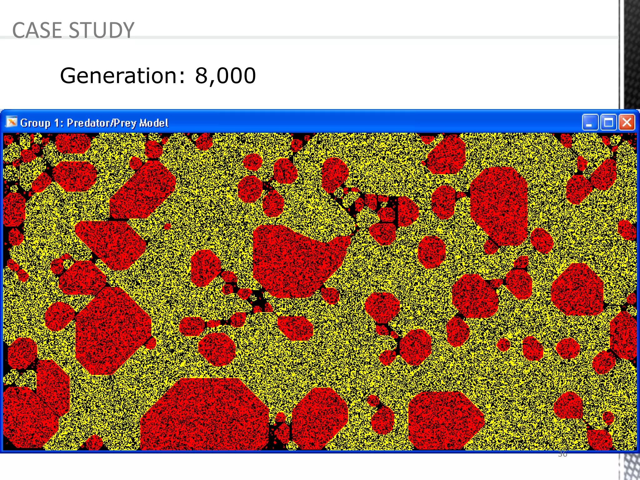
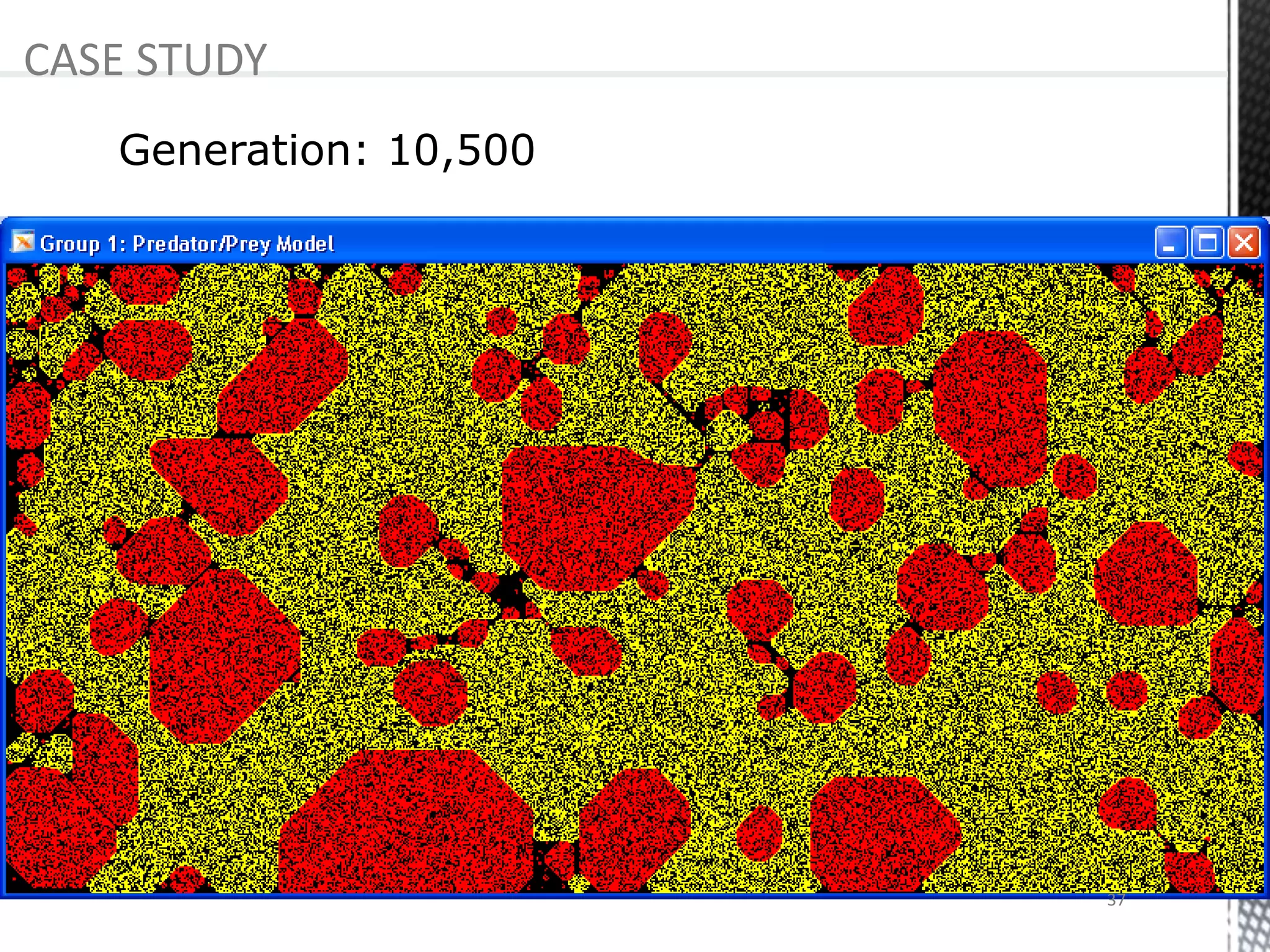


The presentation provides an overview of cellular automata (CA), which are discrete dynamic systems that simulate complex behaviors through simple rules and interactions among cells. It discusses the components, variants, advantages, and disadvantages of CAs, as well as various applications including modeling biological systems and complex phenomena. Case studies illustrate the behavior of CAs in scenarios like predator-prey relationships and forest fire modeling.