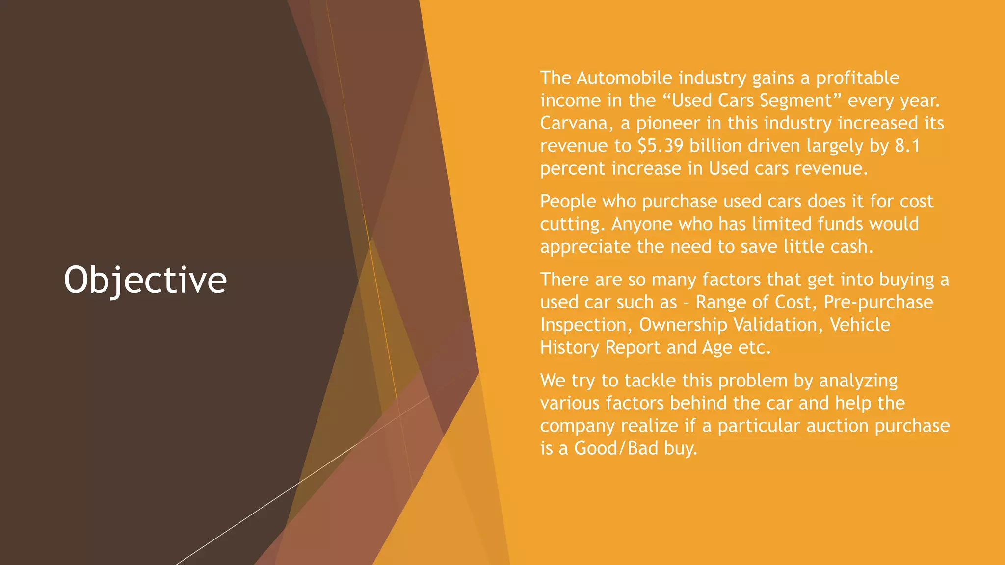
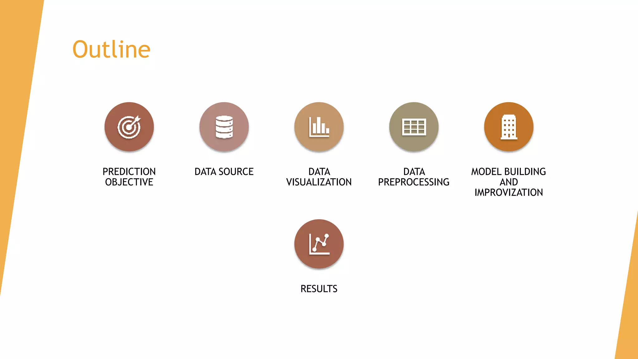
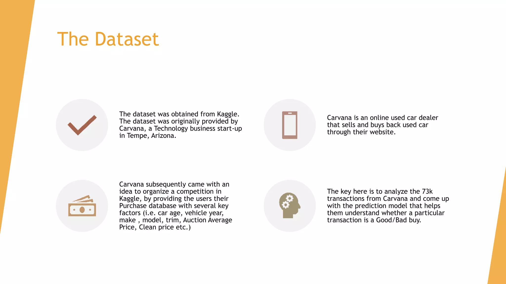
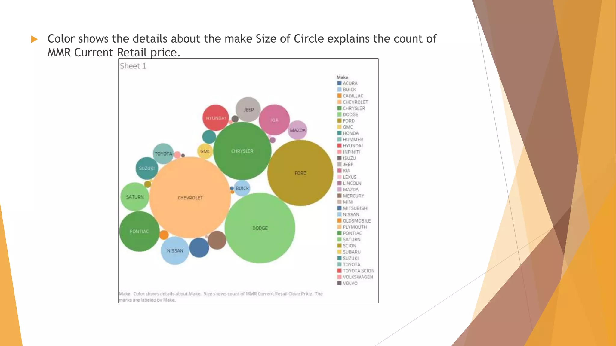
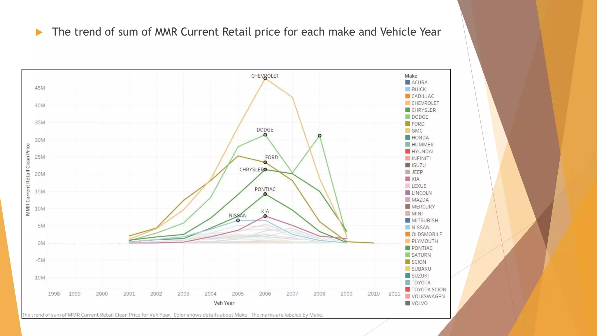
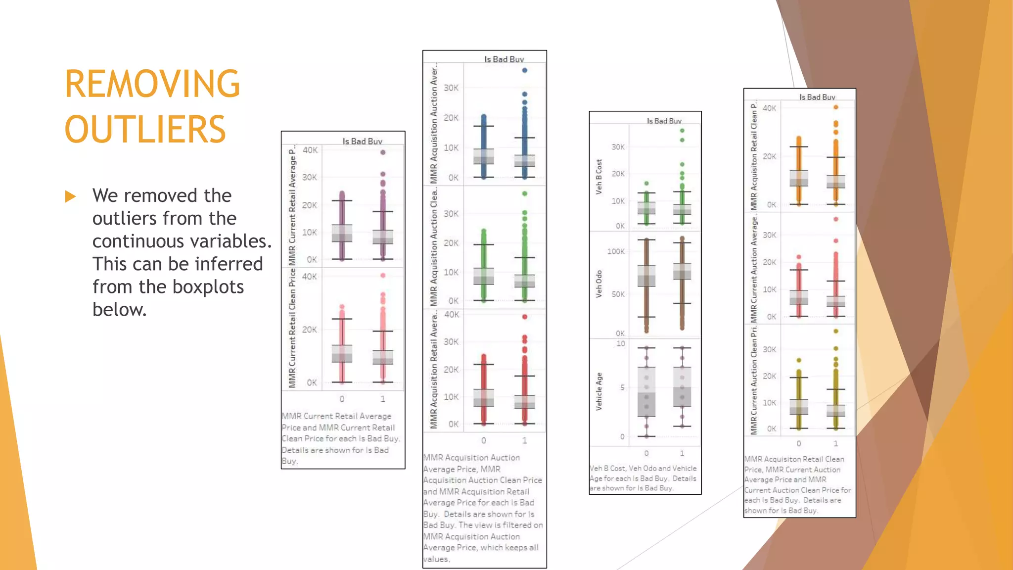
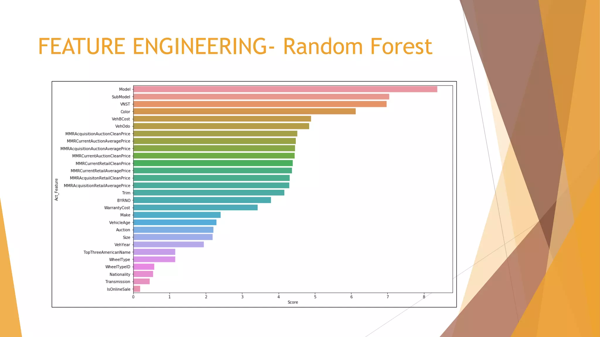
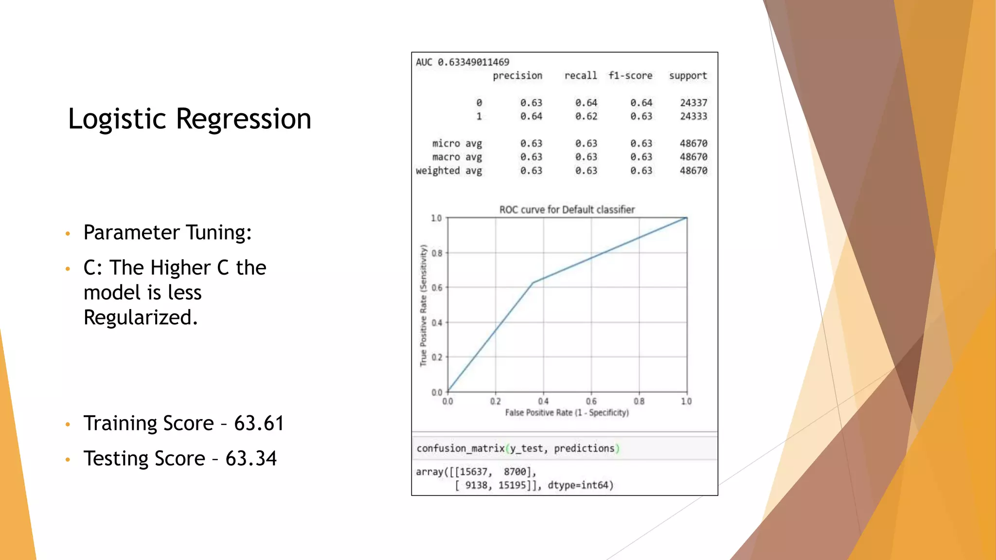
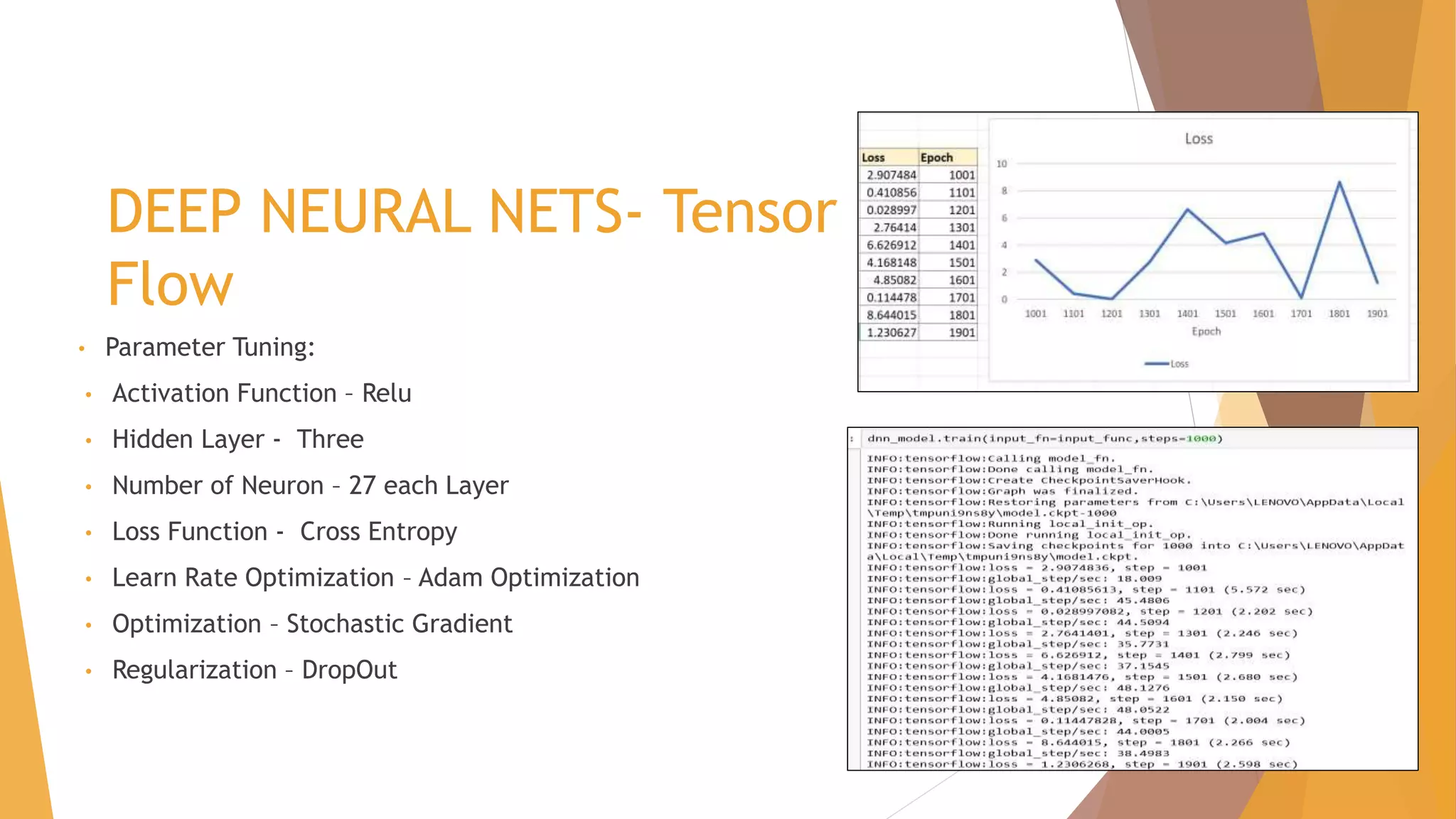
The document outlines Carvana's efforts to enhance their auction purchase predictions in the used car market, leveraging data analysis of 73,000 transactions. It highlights key factors influencing used car purchases and the methodology, including data preprocessing, feature engineering, and various machine learning models used for predictions. The analysis reveals challenges such as class imbalance and model tuning, ultimately presenting training and testing scores for multiple algorithms employed in the study.

1. CARVANA –
Predicting the
Purchase quality
in Car Auction

2. Objective
 The Automobile industry gains a profitable
income in the “Used Cars Segment” every year.
Carvana, a pioneer in this industry increased its
revenue to $5.39 billion driven largely by 8.1
percent increase in Used cars revenue.
 People who purchase used cars does it for cost
cutting. Anyone who has limited funds would
appreciate the need to save little cash.
 There are so many factors that get into buying a
used car such as – Range of Cost, Pre-purchase
Inspection, Ownership Validation, Vehicle
History Report and Age etc.
 We try to tackle this problem by analyzing
various factors behind the car and help the
company realize if a particular auction purchase
is a Good/Bad buy.

3. Outline
PREDICTION
OBJECTIVE
DATA SOURCE DATA
VISUALIZATION
DATA
PREPROCESSING
MODEL BUILDING
AND
IMPROVIZATION
RESULTS

5. The Dataset
The dataset was obtained from Kaggle.
The dataset was originally provided by
Carvana, a Technology business start-up
in Tempe, Arizona.
Carvana is an online used car dealer
that sells and buys back used car
through their website.
Carvana subsequently came with an
idea to organize a competition in
Kaggle, by providing the users their
Purchase database with several key
factors (i.e. car age, vehicle year,
make , model, trim, Auction Average
Price, Clean price etc.)
The key here is to analyze the 73k
transactions from Carvana and come up
with the prediction model that helps
them understand whether a particular
transaction is a Good/Bad buy.

6. DATASET
DESCRIPTION
 The dataset had a total of 34 attributes.
 ReId – This is a Reference Id for each transaction in the
dataset
 PurchDate – Date attribute that specifies the date of
Pruchase.
 Auction – The Auction was help by two groups ADESA and
MANHEIM. Other 3rd party dealers were also involved.
 VehYear – The Year to which a particular model belongs.
 VehicleAge – Number of years the vehicle is used.
 Make – The vehicle company i.e. MAZDA, DODGE, FORD
etc.
 Model – Subclass from each Make i.e. FORD FOCUS,
TOYOTA COROLLA etc.
 Trim – The class distinction in each mode i.e ST, SXT, EX,
SE etc.
 SubModel – This is the type of Model i.e. 4D SEDAN, 2D
COUPE, 4D SUV etc.
 Color – Color of the vehicle
 Transmission – AUTO or MANUAL

7. CONTD..
 WheelTypeID – ID of different types of Wheel
 WheelType – Type of wheel such as ALLOY, COVERS
etc.
 VEhOdo – Number of miles driven
 Nationality – Make’s Nationality
 Size – LARGE TRUCK, MEDIUM SUV etc.
 TopThreeAmericanName – The original parent
company that owns the Make ex- CHRYSLER,
GENERAL MOTORS
MMR refers to the Manheim Market report prices
 MMRAcquisitionAuctionAveragePrice – Acquisition
price for this vehicle in average condition during
purchase
 MMRAcquisitionAuctionCleanPrice - Acquisition price
for this vehicle in the above average condition
during purchase
 MMRAcquisitionRetailAveragePrice- Acquisition price
for this vehicle in retail market in average
condition
 MMRAcquisitonRetailCleanPrice- Acquisition price for
this vehicle in above average condition in the
retail market

8. CONTD..
 MMRCurrentAuctionAveragePrice – The current auction
price for this vehicle in average condition
 MMRCurrentAuctionCleanPrice – The current auction
price of this vehicle in above average condition
 MMRCurrentRetailAveragePrice - The current retail
price for this vehicle in average condition
 MMRCurrentRetailCleanPrice - – The current retail price
for this vehicle in above average condition
 PRIMEUNIT – Identify if the vehicle would have a higher
demand than the standard purchase
 AUCGUART – The guarantee level provided by the auction
for the vehicle
 BYRNO - The ID associated with each buyer
 VNZIP1 - The zip code where the car was purchased
 VNST – The state where the car was purchased
 VehBCost – The initial base price for the vehicle at
beginning of auction
 IsOnlineSale- Whether the car was sold online or not
 WarrantyCost- The cost of warranty for each vehicle

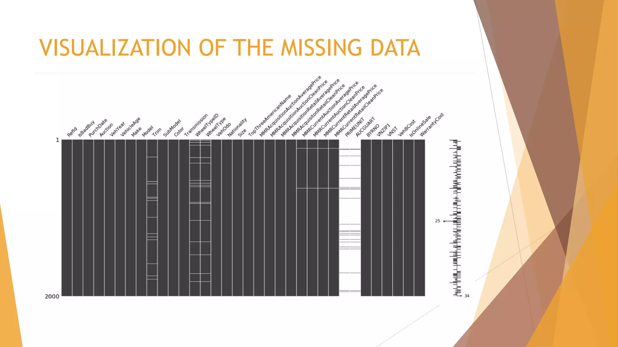
9. Dataset – Initial analysis
 The dataset initially had 34 attributes with the target attribute being – IsBadBuy
 The dataset had 19 numerical attributes and 15 categorical attributes and the
shape and column can be seen below.
CATEGORICAL:
((72983, 15),
Index(['PurchDate', 'Auction', 'Make', 'Model', 'Trim', 'SubModel', 'Color',
'Transmission', 'WheelType', 'Nationality', 'Size',
'TopThreeAmericanName', 'PRIMEUNIT', 'AUCGUART', 'VNST'],
dtype='object’))

10. CONTD…
NUMERIC:
((72983, 19),
Index(['RefId', 'IsBadBuy', 'VehYear', 'VehicleAge', 'WheelTypeID', 'VehOdo',
'MMRAcquisitionAuctionAveragePrice', 'MMRAcquisitionAuctionCleanPrice',
'MMRAcquisitionRetailAveragePrice', 'MMRAcquisitonRetailCleanPrice',
'MMRCurrentAuctionAveragePrice', 'MMRCurrentAuctionCleanPrice',
'MMRCurrentRetailAveragePrice', 'MMRCurrentRetailCleanPrice', 'BYRNO',
'VNZIP1', 'VehBCost', 'IsOnlineSale', 'WarrantyCost'],
dtype='object'))

11. VISUALIZATION OF THE MISSING DATA

12. PROBLEMS FACED -
MISSING VALUES
 The Initial analysis showed that the
dataset had 19 Attributes with
missing values. The statistics for the
missing values are.
 Attributes PRIMEUNIT and ACGUART
had only less than 1% percent of
data and did not help enough with
model building and were removed in
the analysis.
ATTRIBUTE NAME
MISSING
VALUES
Trim 2360
SubModel 8
Color 8
Transmission 9
WheelTypeID 3169
WheelType 3174
Nationality 5
Size 5
TopThreeAmericanName 5
MMRAcquisitionAuctionAveragePrice 18
MMRAcquisitionAuctionCleanPrice 18
MMRAcquisitionRetailAveragePrice 18
MMRAcquisitonRetailCleanPrice 18
MMRCurrentAuctionAveragePrice 315
MMRCurrentAuctionCleanPrice 315
MMRCurrentRetailAveragePrice 315
MMRCurrentRetailCleanPrice 315
PRIMEUNIT 69564
AUCGUART 69564

13. NULLITY CORRELATION FOR MISSING
VALUES

14. PROBLEM FACED –
Class Imbalance
 The original dataset is highly
class imbalanced
 Only 10 percent of the
transaction were a BAD buy and
the rest were GOOD buy

15. CORRELATION MATRIX HEATMAP

16. DATA VISUALIZATION

17. Vehicle year for each make. Color shows the average age of vehicle

18. The number of Cars purchased by the Auction Company vs Make of Car Purchased
by Nationality

19.  Color shows the details about the make Size of Circle explains the count of
MMR Current Retail price.

20.  Color shows the average of current retail price in each
state
 In Second graph Color shows the Average Age of
vehicle in each state

21.  The trend of sum of MMR Current Retail price for each make and Vehicle Year

22. DATA PREPROCESSING

23. REMOVING THE INSIGNIFICANT FEATURES
 The attributes PRIMEUNIT and AUCGUART had less than 1 percent of data and
were found inefficient in predicting the target variable.
 The preliminary data analysis showed that we had 15 Categorical variables.
Now after removing the above 2 features we are left with 13 Categorical
variables now.
 We used One-hot Encoder to create dummy values for the Categorical
variables.

24. CONTD..
 We also removed the numerical variables VNZIP1 and RefId.
 VNZIP1 was jus the zip codes of where the cars were sold. This is redundant
because, we can infer this from the variable VNST(state codes). RefId is just
a transaction ID which had no meaning.

25. REMOVING
OUTLIERS
 We removed the
outliers from the
continuous variables.
This can be inferred
from the boxplots
below.

26. DISTRIBUTION PLOTS
We used distribution plots to check the normality of the continuous variables.

27. SMOTE FOR CLASS IMBALANCE
We used SMOTE technique to solve the class imbalance problem.

28. STANDARDIZATION
OF FEATURES
USING SCALING
 We used Standard
Scalar to perform
standardization so that
all the numerical
variables fall in the
same scale throughout
the dataset.

29. FEATURE ENGINEERING- Random Forest

30. MACHINE LEARNING
MODELS

31. Random
Forest
 Version:
 Original Data
 SMOTE+ RF
 Oversampling+ RF
 Under Sample+ RF
 Parameter Tuning:
 n_estimators
 Criterion
 max_depth
 max_feature

32. Random -Under Sampling Random – Over Sampling Over Sampling – SMOTE

33. K Nearest
Neighbor
• Parameter Tuning:
• N_Neighbors
• Distance Measure
• a. p=0 Minkowski
• b. p=1 Manhantan
• c. p=2 Eulidean

34. KNN – Report
Training Score – 90.4
Testing Score – 90.5

35. Ensemblem –
Ada Boosting
 Parameter Tuning
 Weak Learning – Decision Tree
 criterion = “entropy”
 Max_depth = 5
 Random_state
 Algorithm= SAME.R – Real
Boosting
 Train Score: 92.50
 Test Score: 75.65

36. K Fold Cross Validation – Ada Boosting

37. Logistic Regression
• Parameter Tuning:
• C: The Higher C the
model is less
Regularized.
• Training Score – 63.61
• Testing Score – 63.34

38. DEEP NEURAL NETS- Tensor
Flow
• Parameter Tuning:
• Activation Function – Relu
• Hidden Layer - Three
• Number of Neuron – 27 each Layer
• Loss Function - Cross Entropy
• Learn Rate Optimization – Adam Optimization
• Optimization – Stochastic Gradient
• Regularization – DropOut

39. DNN – Report

40. PCA – Principal
Component Analysis
 Parameter Tuning
 Number of Components --- Elbow plot
 Explained variance vs Number of components


41. PCA- COMPONENTS FEATURE VARIANCE

42. PCA+SMOTE+RF

43. CHALLENGES FACED – Algorithm
SVM
 Parameter Tuning
 C , gamma , Kernal.
 Grid Search
 C=[0.1,1,10,100]
 Gamma=[1,0.1,0.01,0.0001]
 Kernel- rbf.
 Time Execution – More than 12
hours , for 25 fits out of 75 fits

44. Challenges Faced – Data
 Data Imblance – Random Over Sampling, Random Under Sampling, SMOTE.
 Distribution of Continous Variable – Applied Log Transformation
 Over Fitting – K fold cross validation, HyperParameter Tuning.
 Dimensionality – PCA

45. SUMMARY
Model Train Score
Tesing
Score Precision Recal AUC
Knn+SMOTE 90.4 90.5 0.84 0.9 0.5
RF 75 50 0.65 0.45 0.5
RF+ UnderSample 65.3 63 0.63 0.63 0.63
RF+ OverSample 63.9 63.3 0.63 0.63 0.63
RF+Over Sampling
SMOTE 87.6 87.5 0.88 0.88 0.875
Ada Boosting 92.5 75.65 0.75 0.75 0.74
DNN 94.5 95.4 0.84 0.9 0.9
Logisti Regression 63.61 63.64 0.63 0.63 0.633
PCA+SMOTE+RF 76.5 76.5 0.76 0.8 0.76