Download to read offline
![Step 0: Selection & Reproducibility
As Machine Learning gains attention, more applications and models are being used, and often speed or
accuracy of the predicted models lack comparisons. In this analysis, we’ll compare the accuracy and speed
of 20 Machine learning models commonly selected. We’ll exercise these models on two multinomial UCI
reference datasets, differing in size, predictor levels and number of dependent variables. The first and smallest
dataset is Car_Evaluation and we’ll compare results when applying on the larger and more complex Nursery
dataset.
Sys.info()[1:5]
## sysname release version nodename machine
## "Windows" "10 x64" "build 10586" "STALLION" "x86-64"
sessionInfo()
## R version 3.2.4 Revised (2016-03-16 r70336)
## Platform: x86_64-w64-mingw32/x64 (64-bit)
## Running under: Windows 10 x64 (build 10586)
##
## locale:
## [1] LC_COLLATE=English_United States.1252
## [2] LC_CTYPE=English_United States.1252
## [3] LC_MONETARY=English_United States.1252
## [4] LC_NUMERIC=C
## [5] LC_TIME=English_United States.1252
##
## attached base packages:
## [1] stats graphics grDevices utils datasets methods base
##
## loaded via a namespace (and not attached):
## [1] magrittr_1.5 formatR_1.3 tools_3.2.4 htmltools_0.3
## [5] yaml_2.1.13 stringi_1.0-1 rmarkdown_0.9.5 knitr_1.12.3
## [9] stringr_1.0.0 digest_0.6.9 evaluate_0.8.3
library(stringr)
library(knitr)
userdir <- getwd()
set.seed(123)
Step 1: Retrieve 1st Dataset
We will mirror the approach used in the formulation challenge and use first the Car Evaluation dataset hosted
on UCI Machine Learning Repository. We will use R to reproducibly and quickly download the dataset, and
its full description. We continue to maintain reproducibility of the analysis as a general practice. The analysis
tool and platform are documented, all libraries clearly listed, while data is retrieved programmatically and
date stamped from the repository.
We will display a structure of the Car_Evaluation dataset and the corresponding dictionary to translate the
attribute factors.
2](https://image.slidesharecdn.com/c82e6671-3f33-414c-b7f8-10d708a95260-160405142034/85/Benchmarking_ML_Tools-2-320.jpg)
![datadir <- "./data"
if (!file.exists("data")){dir.create("data")}
uciUrl <- "http://archive.ics.uci.edu/ml/machine-learning-databases/"
fileUrl <- paste0(uciUrl,"car/car.data?accessType=DOWNLOAD")
download.file(fileUrl, destfile="./data/cardata.csv", method = "curl")
dateDownloaded <- date()
car_eval <- read.csv("./data/cardata.csv",header=FALSE)
fileUrl <- paste0(uciUrl,"car/car.names?accessType=DOWNLOAD")
download.file(fileUrl, destfile = "./data/carnames.txt")
txt <- readLines("./data/carnames.txt")
lns <- data.frame(beg=which(grepl("buying v-high",txt)),end=which(grepl("med, high",txt)))
# we now capture all lines of text between beg and end from txt
res <- lapply(seq_along(lns$beg),function(l){paste(txt[seq(from=lns$beg[l],to=lns$end[l],by=1)],collapse
res <- gsub(" ", ":", res, fixed = TRUE)
res <- gsub(" ", ":", res, fixed = TRUE)
res <- gsub(" ", ":", res, fixed = TRUE)
res <- gsub(" ", ":", res, fixed = TRUE)
res <- gsub(" ", "n", res, fixed = TRUE)
res <- gsub(" ", "", res, fixed = TRUE)
res <- gsub(" ", "", res, fixed = TRUE)
res <- str_c(res,"n")
writeLines(res, "./data/parsed_attr.csv")
attrib <- readLines("./data/parsed_attr.csv")
nv <- length(attrib) # number of attributes
attrib <- sapply (1:nv,function(i) {gsub(":"," ",attrib[i],fixed=TRUE)})
dictionary <- sapply (1:nv,function(i) {strsplit(attrib[i],' ')})
dictionary[[nv]][1]<-"class"
colnames(car_eval)<-sapply(1:nv,function(i) {colnames(car_eval)[i]<-dictionary[[i]][1]})
cm<-list()
x<-car_eval[,1:(nv-1)]
y<-car_eval[,nv]
fmla<-paste(colnames(car_eval)[1:(nv-1)],collapse="+")
fmla<-paste0(colnames(car_eval)[nv],"~",fmla)
fmla<-as.formula(fmla)
nlev<-nlevels(y) # number of factors describing class
Step 2. Data Exploration
head(car_eval)
## buying maint doors persons lug_boot safety class
## 1 vhigh vhigh 2 2 small low unacc
## 2 vhigh vhigh 2 2 small med unacc
## 3 vhigh vhigh 2 2 small high unacc
## 4 vhigh vhigh 2 2 med low unacc
## 5 vhigh vhigh 2 2 med med unacc
## 6 vhigh vhigh 2 2 med high unacc
summary(car_eval)
## buying maint doors persons lug_boot safety
3](https://image.slidesharecdn.com/c82e6671-3f33-414c-b7f8-10d708a95260-160405142034/85/Benchmarking_ML_Tools-3-320.jpg)
![## high :432 high :432 2 :432 2 :576 big :576 high:576
## low :432 low :432 3 :432 4 :576 med :576 low :576
## med :432 med :432 4 :432 more:576 small:576 med :576
## vhigh:432 vhigh:432 5more:432
## class
## acc : 384
## good : 69
## unacc:1210
## vgood: 65
str(car_eval)
## 'data.frame': 1728 obs. of 7 variables:
## $ buying : Factor w/ 4 levels "high","low","med",..: 4 4 4 4 4 4 4 4 4 4 ...
## $ maint : Factor w/ 4 levels "high","low","med",..: 4 4 4 4 4 4 4 4 4 4 ...
## $ doors : Factor w/ 4 levels "2","3","4","5more": 1 1 1 1 1 1 1 1 1 1 ...
## $ persons : Factor w/ 3 levels "2","4","more": 1 1 1 1 1 1 1 1 1 2 ...
## $ lug_boot: Factor w/ 3 levels "big","med","small": 3 3 3 2 2 2 1 1 1 3 ...
## $ safety : Factor w/ 3 levels "high","low","med": 2 3 1 2 3 1 2 3 1 2 ...
## $ class : Factor w/ 4 levels "acc","good","unacc",..: 3 3 3 3 3 3 3 3 3 3 ...
cm<-list() # initialize
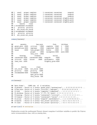
Exploration reveals the multinomial car experience dataset comprises 6 attributes factors we can use to
predict the 4-factor car recommendation class, with no missing data.
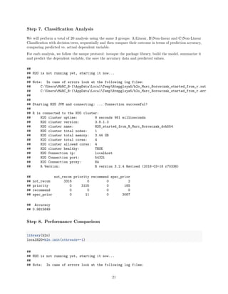
Step 3. Classification Analysis
20 Models will be sequentially selected to represent 3 groups: A)Linear, B)Non-linear and C)Non-Linear
Classification with decision trees. From the collected Confusion Matrix performance, we will build a results
data frame and compare the prediction accuracies.
For each analysis, we’ll follow the sampe protocol: invoque the package library, build the model, summarize
it and predict the class (dependent variable), then save the accuracy data and predicted values in a list.
3.A Linear Classification
3.A1 Multinomial
library(nnet)
library(caret)
model<-multinom(fmla, data = car_eval, maxit = 500, trace=FALSE)
prob<-predict(model,x,type="probs")
pred<-apply(prob,1,which.max)
pred[which(pred=="1")]<-levels(y)[1]
pred[which(pred=="2")]<-levels(y)[2]
pred[which(pred=="3")]<-levels(y)[3]
pred[which(pred=="4")]<-levels(y)[4]
pred<-as.factor(pred)
l<-union(pred,y)
mtab<-table(factor(pred,l),factor(y,l))
cm[[1]]<-c("Multinomial","MULTINOM",confusionMatrix(mtab))
cm[[1]]$table
4](https://image.slidesharecdn.com/c82e6671-3f33-414c-b7f8-10d708a95260-160405142034/85/Benchmarking_ML_Tools-4-320.jpg)
![##
## unacc acc vgood good
## unacc 1166 32 0 0
## acc 43 346 2 6
## vgood 0 2 63 4
## good 1 4 0 59
cm[[1]]$overall[1]
## Accuracy
## 0.9456019
3.A2 Logistic Regression
library(VGAM)
model<-vglm(fmla, family = "multinomial", data = car_eval, maxit = 100)
prob<-predict(model,x,type="response")
pred<-apply(prob,1,which.max)
pred[which(pred=="1")]<-levels(y)[1]
pred[which(pred=="2")]<-levels(y)[2]
pred[which(pred=="3")]<-levels(y)[3]
pred[which(pred=="4")]<-levels(y)[4]
pred<-as.factor(pred)
l<-union(pred,y)
mtab<-table(factor(pred,l),factor(y,l))
cm[[2]]<-c("Logistic Regression","GLM",confusionMatrix(mtab))
cm[[2]]$table
##
## unacc acc vgood good
## unacc 1166 32 0 0
## acc 43 346 2 6
## vgood 0 2 63 4
## good 1 4 0 59
cm[[2]]$overall[1]
## Accuracy
## 0.9456019
3.A3 Linear Discriminant Analysis
library(MASS)
model<-lda(fmla,data=car_eval)
pred<-predict(model,x)$class
l<-union(pred,y)
mtab<-table(factor(pred,l),factor(y,l))
cm[[3]]<-c("Linear Discriminant Analysis","LDA",confusionMatrix(mtab))
cm[[3]]$table
5](https://image.slidesharecdn.com/c82e6671-3f33-414c-b7f8-10d708a95260-160405142034/85/Benchmarking_ML_Tools-5-320.jpg)
![##
## unacc acc vgood good
## unacc 1138 13 0 0
## acc 70 361 27 44
## vgood 0 0 35 2
## good 2 10 3 23
cm[[3]]$overall[1]
## Accuracy
## 0.9010417
3.B Non-Linear Classification
3.B1 Mixture Discriminant Analysis
library(mda)
model<-mda(fmla,data=car_eval)
pred<-predict(model,x)
l<-union(pred,y)
mtab<-table(factor(pred,l),factor(y,l))
cm[[4]]<-c("Mixture Discriminant Analysis","MDA",confusionMatrix(mtab))
cm[[4]]$table
##
## unacc acc vgood good
## unacc 1151 16 0 0
## acc 52 341 7 21
## vgood 0 4 55 3
## good 7 23 3 45
cm[[4]]$overall[1]
## Accuracy
## 0.9212963
3.B2 Regularized Discriminant Analysis
library(klaR)
model<-rda(fmla,data=car_eval,gamma = 0.05,lambda = 0.01)
pred<-predict(model,x)$class
l<-union(pred,y)
mtab<-table(factor(pred,l),factor(y,l))
cm[[5]]<-c("Regularized Discriminant Analysis","RDA",confusionMatrix(mtab))
cm[[5]]$table
##
## unacc acc vgood good
## unacc 1072 0 0 0
## acc 134 317 0 0
## vgood 0 22 65 6
## good 4 45 0 63
6](https://image.slidesharecdn.com/c82e6671-3f33-414c-b7f8-10d708a95260-160405142034/85/Benchmarking_ML_Tools-6-320.jpg)
![cm[[5]]$overall[1]
## Accuracy
## 0.8778935
3.B3 Neural Network
library(nnet)
library(devtools)
model<-nnet(fmla,data=car_eval,size = 4, decay = 0.0001, maxit = 700, trace = FALSE)
#import the function from Github
# source_url('https://gist.githubusercontent.com/Peque/41a9e20d6687f2f3108d/raw/85e14f3a292e126f14548644
# plot.nnet(model, alpha.val = 0.5, cex= 0.7, circle.col = list('lightblue', 'white'), bord.col = 'black
pred<-predict(model,x,type="class")
pred<-as.factor(pred)
l<-union(pred,y)
mtab<-table(factor(pred,l),factor(y,l))
cm[[6]]<-c("Neural Network","NNET",confusionMatrix(mtab))
cm[[6]]$table
##
## unacc acc vgood good
## unacc 1208 2 0 0
## acc 2 376 0 6
## vgood 0 0 64 1
## good 0 6 1 62
cm[[6]]$overall[1]
## Accuracy
## 0.9895833
3.B4 Flexible Discriminant Analysis
library(mda)
model<-fda(fmla,data=car_eval)
pred<-predict(model,x,type="class")
l<-union(pred,y)
mtab<-table(factor(pred,l),factor(y,l))
cm[[7]]<-c("Flexible Discriminant Analysis","FDA",confusionMatrix(mtab))
cm[[7]]$table
##
## unacc acc vgood good
## unacc 1136 13 0 0
## acc 72 361 27 44
## vgood 0 0 35 2
## good 2 10 3 23
7](https://image.slidesharecdn.com/c82e6671-3f33-414c-b7f8-10d708a95260-160405142034/85/Benchmarking_ML_Tools-7-320.jpg)
![cm[[7]]$overall[1]
## Accuracy
## 0.8998843
3.B5 Support Vector Machine
library(kernlab)
model<-ksvm(fmla,data=car_eval)
pred<-predict(model,x,type="response")
l<-union(pred,y)
mtab<-table(factor(pred,l),factor(y,l))
cm[[8]]<-c("Support Vector Machine","SVM",confusionMatrix(mtab))
cm[[8]]$table
##
## unacc acc vgood good
## unacc 1174 0 0 0
## acc 33 375 0 0
## vgood 0 1 65 9
## good 3 8 0 60
cm[[8]]$overall[1]
## Accuracy
## 0.96875
3.B6 k-Nearest Neighbors
library(caret)
model<-knn3(fmla,data=car_eval,k=nlev+1)
pred<-predict(model,x,type="class")
l<-union(pred,y)
mtab<-table(factor(pred,l),factor(y,l))
cm[[9]]<-c("k-Nearest Neighbors","KNN",confusionMatrix(mtab))
cm[[9]]$table
##
## unacc acc good vgood
## unacc 1199 41 4 1
## acc 11 336 45 15
## good 0 6 15 4
## vgood 0 1 5 45
cm[[9]]$overall[1]
## Accuracy
## 0.9230324
8](https://image.slidesharecdn.com/c82e6671-3f33-414c-b7f8-10d708a95260-160405142034/85/Benchmarking_ML_Tools-8-320.jpg)
![3.B8 Naive Bayes
library(e1071)
model<-naiveBayes(fmla,data=car_eval,k=nlev+1)
pred<-predict(model,x)
l<-union(pred,y)
mtab<-table(factor(pred,l),factor(y,l))
cm[[10]]<-c("Naive Bayes","NBAYES",confusionMatrix(mtab))
cm[[10]]$table
##
## unacc acc vgood good
## unacc 1161 85 0 0
## acc 47 289 26 46
## vgood 0 0 39 2
## good 2 10 0 21
cm[[10]]$overall[1]
## Accuracy
## 0.8738426
3.C Non-Linear Classification with Decision Trees
3.C1 Classification and Regression Trees(CART)
library(rpart)
library(rpart.plot)
model<-rpart(fmla,data=car_eval)
# prp(model, faclen=3)
pred<-predict(model, x ,type="class")
l<-union(pred,y)
mtab<-table(factor(pred,l),factor(y,l))
cm[[11]]<-c("classification and Regression Trees","CART",confusionMatrix(mtab))
cm[[11]]$table
##
## unacc acc good vgood
## unacc 1161 7 0 0
## acc 45 358 0 13
## good 4 16 60 0
## vgood 0 3 9 52
cm[[11]]$overall[1]
## Accuracy
## 0.9438657
3.C2 OneR
9](https://image.slidesharecdn.com/c82e6671-3f33-414c-b7f8-10d708a95260-160405142034/85/Benchmarking_ML_Tools-9-320.jpg)
![library(RWeka)
model<-OneR(fmla,data=car_eval)
pred<-predict(model,x,type="class")
l<-union(pred,y)
mtab<-table(factor(pred,l),factor(y,l))
cm[[12]]<-c("One R","ONE-R",confusionMatrix(mtab))
cm[[12]]$table
##
## unacc acc vgood good
## unacc 1210 384 65 69
## acc 0 0 0 0
## vgood 0 0 0 0
## good 0 0 0 0
cm[[12]]$overall[1]
## Accuracy
## 0.7002315
3.C3 C4.5
library(RWeka)
model<-J48(fmla,data=car_eval)
pred<-predict(model,x)
l<-union(pred,y)
mtab<-table(factor(pred,l),factor(y,l))
cm[[13]]<-c("C4.5","C45",confusionMatrix(mtab))
cm[[13]]$table
##
## unacc acc vgood good
## unacc 1172 0 0 0
## acc 35 380 4 9
## vgood 0 2 55 3
## good 3 2 6 57
cm[[13]]$overall[1]
## Accuracy
## 0.962963
3.C4 PART
library(RWeka)
model<-PART(fmla,data=car_eval)
pred<-predict(model,x)
l<-union(pred,y)
mtab<-table(factor(pred,l),factor(y,l))
cm[[14]]<-c("PART","PART",confusionMatrix(mtab))
cm[[14]]$table
10](https://image.slidesharecdn.com/c82e6671-3f33-414c-b7f8-10d708a95260-160405142034/85/Benchmarking_ML_Tools-10-320.jpg)
![##
## unacc acc vgood good
## unacc 1196 6 0 1
## acc 13 374 0 3
## vgood 0 3 65 2
## good 1 1 0 63
cm[[14]]$overall[1]
## Accuracy
## 0.9826389
3.C5 Bagging CART
library(ipred)
model<-bagging(fmla,data=car_eval)
pred<-predict(model,x)
l<-union(pred,y)
mtab<-table(factor(pred,l),factor(y,l))
cm[[15]]<-c("Bagging CART","BAG-CART",confusionMatrix(mtab))
cm[[15]]$table
##
## unacc acc vgood good
## unacc 1210 0 0 0
## acc 0 384 0 0
## vgood 0 0 65 0
## good 0 0 0 69
cm[[15]]$overall[1]
## Accuracy
## 1
3.C6 Random Forest
library(randomForest)
model<-randomForest(fmla,data=car_eval)
pred<-predict(model,x)
l<-union(pred,y)
mtab<-table(factor(pred,l),factor(y,l))
cm[[16]]<-c("Random Forest","RF",confusionMatrix(mtab))
cm[[16]]$table
##
## unacc acc vgood good
## unacc 1208 0 0 0
## acc 2 384 0 0
## vgood 0 0 65 0
## good 0 0 0 69
11](https://image.slidesharecdn.com/c82e6671-3f33-414c-b7f8-10d708a95260-160405142034/85/Benchmarking_ML_Tools-11-320.jpg)
![cm[[16]]$overall[1]
## Accuracy
## 0.9988426
3.C7 Gradient Boosted Machine
library(gbm)
model<-gbm(fmla,data=car_eval,n.trees=5000,interaction.depth=nlev,shrinkage=0.001,bag.fraction=0.8,distr
prob<-predict(model,x,n.trees=5000,type="response")
pred<-apply(prob,1,which.max)
pred[which(pred=="1")]<-levels(y)[1]
pred[which(pred=="2")]<-levels(y)[2]
pred[which(pred=="3")]<-levels(y)[3]
pred[which(pred=="4")]<-levels(y)[4]
pred<-as.factor(pred)
l<-union(pred,y)
mtab<-table(factor(pred,l),factor(y,l))
cm[[17]]<-c("Gradient Boosted Machine","GBM",confusionMatrix(mtab))
cm[[17]]$table
##
## unacc acc vgood good
## unacc 1191 3 0 0
## acc 16 372 1 0
## vgood 0 0 64 4
## good 3 9 0 65
cm[[17]]$overall[1]
## Accuracy
## 0.9791667
3.C8 Boosted C5.0
library(C50)
model<-C5.0(fmla,data=car_eval,trials=10)
# tree <- rpart(model,data=car_eval,control=rpart.control(minsplit=20,cp=0,digits=6))
# prp(tree,faclen=3)
pred<-predict(model,x)
l<-union(pred,y)
mtab<-table(factor(pred,l),factor(y,l))
cm[[18]]<-c("Boosted C5.0","BOOST-C50",confusionMatrix(mtab))
cm[[18]]$table
##
## unacc acc vgood good
## unacc 1207 1 0 0
## acc 3 383 2 0
## vgood 0 0 63 0
## good 0 0 0 69
12](https://image.slidesharecdn.com/c82e6671-3f33-414c-b7f8-10d708a95260-160405142034/85/Benchmarking_ML_Tools-12-320.jpg)
![cm[[18]]$overall[1]
## Accuracy
## 0.9965278
3.C9 JRip
library(RWeka)
model<-JRip(fmla,data=car_eval)
pred<-predict(model,x)
l<-union(pred,y)
mtab<-table(factor(pred,l),factor(y,l))
cm[[19]]<-c("JRip","JRIP",confusionMatrix(mtab))
cm[[19]]$table
##
## unacc acc vgood good
## unacc 1156 0 0 0
## acc 44 356 2 6
## vgood 4 16 61 3
## good 6 12 2 60
cm[[19]]$overall[1]
## Accuracy
## 0.9450231
3.C10 H2O Deep Learning
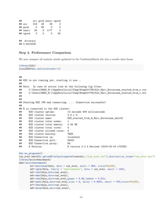
##
## H2O is not running yet, starting it now...
##
## Note: In case of errors look at the following log files:
## C:UsersMARC_B~1AppDataLocalTempRtmpglsya5/h2o_Marc_Borowczak_started_from_r.out
## C:UsersMARC_B~1AppDataLocalTempRtmpglsya5/h2o_Marc_Borowczak_started_from_r.err
##
##
## Starting H2O JVM and connecting: ... Connection successful!
##
## R is connected to the H2O cluster:
## H2O cluster uptime: 9 seconds 10 milliseconds
## H2O cluster version: 3.8.1.3
## H2O cluster name: H2O_started_from_R_Marc_Borowczak_dvn595
## H2O cluster total nodes: 1
## H2O cluster total memory: 3.44 GB
## H2O cluster total cores: 4
## H2O cluster allowed cores: 4
## H2O cluster healthy: TRUE
## H2O Connection ip: localhost
## H2O Connection port: 54321
## H2O Connection proxy: NA
## R Version: R version 3.2.4 Revised (2016-03-16 r70336)
13](https://image.slidesharecdn.com/c82e6671-3f33-414c-b7f8-10d708a95260-160405142034/85/Benchmarking_ML_Tools-13-320.jpg)
![m9<-knn3(fmla,data=car_eval,k=nlev+1),
m10<-naiveBayes(fmla,data=car_eval,k=nlev+1),
m11<-rpart(fmla,data=car_eval),
m12<-OneR(fmla,data=car_eval),
m13<-J48(fmla,data=car_eval),
m14<-PART(fmla,data=car_eval),
m15<-bagging(fmla,data=car_eval),
m16<-randomForest(fmla,data=car_eval),
m17<-gbm(fmla,data=car_eval,n.trees=5000,interaction.depth=nlev,shrinkage=0.001,bag.fraction=0.8
m18<-C5.0(fmla,data=car_eval,trials=10),
m19<-JRip(fmla,data=car_eval),
m20<-h2o.deeplearning(x=1:(nv-1), y=nv, training_frame = car_eval.hex, variable_importances = TR
times=5)
h2o.shutdown(prompt = FALSE)
## [1] TRUE
#
library(dplyr)
models<-length(cm)
mbm$expr<-rep(sapply(1:models, function(i) {cm[[i]][[2]]}),5)
mbm<-aggregate(x=mbm$time,by=list(Model=mbm$expr),FUN=mean)
mbm$x<-mbm$x/min(mbm$x)
results<-sapply (1:models, function(i) {c(cm[[i]][[1]],cm[[i]][[2]],mbm$x[i],cm[[i]]$overall[1:6])})
row.names(results)<-c("Description","Model","Model_Time_X",names(cm[[1]]$overall[1:6]))
results<-as.data.frame(t(results))
results[,3:9]<-sapply(3:9,function(i){results[,i]<-as.numeric(levels(results[,i])[results[,i]])})
results<-results[,-(8:9)]
results<-arrange(results,desc(Accuracy))
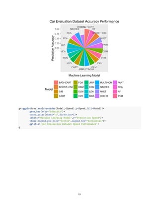
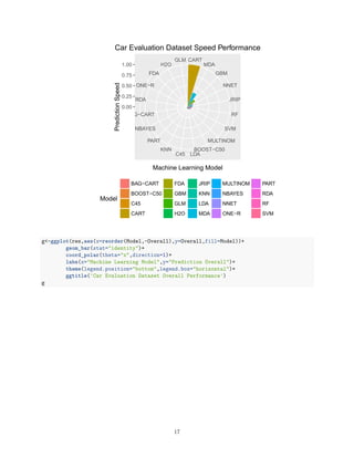
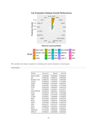
We are now ready to chart on faceted pie charts, with decreasing value order to ease comparisons.
library(ggplot2)
library(gridExtra)
res<-data.frame(Model=results$Model,Accuracy=results$Accuracy,Speed=1/results$Model_Time_X,Overall=resul
library(RColorBrewer)
myPalette <- colorRampPalette(rev(brewer.pal(12, "Set3")))
sc <- scale_colour_gradientn(colours = myPalette(256), limits=c(0.8, 1))
g<-ggplot(res,aes(x=reorder(Model,-Accuracy),y=Accuracy,fill=Model))+
geom_bar(stat="identity")+
coord_polar(theta="x",direction=1)+
labs(x="Machine Learning Model",y="Prediction Accuracy")+
theme(legend.position="bottom",legend.box="horizontal")+
ggtitle('Car Evaluation Dataset Accuracy Performance')
g
15](https://image.slidesharecdn.com/c82e6671-3f33-414c-b7f8-10d708a95260-160405142034/85/Benchmarking_ML_Tools-15-320.jpg)
![Step 5: Retrieve 2nd Dataset
We now repeat with the nursery dataset. Again, We will use R to demonstrate quickly the approach on
this dataset, and its full description. We continue to maintain reproducibility of the analysis as a general
practice. The analysis tool and platform are documented, all libraries clearly listed, while data is retrieved
programmatically and date stamped from the repository.
We will display a structure of the Nursery dataset and the corresponding dictionary to translate the property
factors.
datadir <- "./data"
if (!file.exists("data")){dir.create("data")}
uciUrl <- "http://archive.ics.uci.edu/ml/machine-learning-databases/"
fileUrl <- paste0(uciUrl,"nursery/nursery.data?accessType=DOWNLOAD")
download.file(fileUrl,destfile="./data/nurserydata.csv",method="curl")
dateDownloaded <- date()
nursery <- read.csv("./data/nurserydata.csv",header=FALSE)
fileUrl <- paste0(uciUrl,"nursery/nursery.names?accessType=DOWNLOAD")
download.file(fileUrl,destfile="./data/nurserynames.txt")
txt <- readLines("./data/nurserynames.txt")
lns <- data.frame(beg=which(grepl("parents usual",txt)),end=which(grepl("priority, not_recom",txt
# capture text between beg and end from txt
res <- lapply(seq_along(lns$beg),
function(l){paste(txt[seq(from=lns$beg[l],to=lns$end[l],by=1)],collapse=" ")})
res <- gsub(" ", ":", res, fixed = TRUE)
res <- gsub(" ", ":", res, fixed = TRUE)
res <- gsub(" ", ":", res, fixed = TRUE)
res <- gsub(" ", ":", res, fixed = TRUE)
res <- gsub(" ", "n", res, fixed = TRUE)
res <- gsub(" ", "", res, fixed = TRUE)
res <- gsub(" ", "", res, fixed = TRUE)
res <- gsub(" ", "", res, fixed = TRUE)
res <- str_c(res,"n")
writeLines(res,"./data/n_parsed_attr.csv")
attrib <- readLines("./data/n_parsed_attr.csv")
nv <- length(attrib) # number of attributes
attrib <- sapply (1:nv,function(i) {gsub(":"," ",attrib[i],fixed=TRUE)})
dictionary <- sapply (1:nv,function(i) {strsplit(attrib[i],' ')})
dictionary[[nv]][1]<-"class"
colnames(nursery)<-sapply(1:nv,function(i) {colnames(nursery)[i]<-dictionary[[i]][1]})
x<-nursery[,1:(nv-1)]
y<-nursery[,nv]
fmla<-paste(colnames(nursery)[1:(nv-1)],collapse="+")
fmla<-paste0(colnames(nursery)[nv],"~",fmla)
fmla<-as.formula(fmla)
nlev<-nlevels(y) # number of factors describing class
Step 6. Data Exploration
head(nursery)
## parents has_nurs form children housing finance social
19](https://image.slidesharecdn.com/c82e6671-3f33-414c-b7f8-10d708a95260-160405142034/85/Benchmarking_ML_Tools-19-320.jpg)
![## C:UsersMARC_B~1AppDataLocalTempRtmpUrf7Ob/h2o_Marc_Borowczak_started_from_r.out
## C:UsersMARC_B~1AppDataLocalTempRtmpUrf7Ob/h2o_Marc_Borowczak_started_from_r.err
##
##
## Starting H2O JVM and connecting: .... Connection successful!
##
## R is connected to the H2O cluster:
## H2O cluster uptime: 9 seconds 761 milliseconds
## H2O cluster version: 3.8.1.3
## H2O cluster name: H2O_started_from_R_Marc_Borowczak_gcl376
## H2O cluster total nodes: 1
## H2O cluster total memory: 3.44 GB
## H2O cluster total cores: 4
## H2O cluster allowed cores: 4
## H2O cluster healthy: TRUE
## H2O Connection ip: localhost
## H2O Connection port: 54321
## H2O Connection proxy: NA
## R Version: R version 3.2.4 Revised (2016-03-16 r70336)
h2o.no_progress()
nursery.hex=h2o.uploadFile(path=paste0(userdir,"/nursery.csv"),destination_frame="nursery.hex")
library(microbenchmark)
mbm<-microbenchmark(
m1<-multinom(fmla, data = nursery, maxit = 1200, trace=FALSE),
m2<-vglm(fmla, family = "multinomial", data = nursery, maxit = 100),
m3<-lda(fmla,data=nursery),
m4<-mda(fmla,data=nursery),
m5<-rda(fmla,data=nursery,gamma = 0.05,lambda = 0.01),
m6<-nnet(fmla,data=nursery,size = 4, decay = 0.0001, maxit = 1200,trace=FALSE),
m7<-fda(fmla,data=nursery),
m8<-ksvm(fmla,data=nursery),
m9<-knn3(fmla,data=nursery,k=nlev+1),
m10<-naiveBayes(fmla,data=nursery,k=nlev+1),
m11<-rpart(fmla,data=nursery),
m12<-OneR(fmla,data=nursery),
m13<-J48(fmla,data=nursery),
m14<-PART(fmla,data=nursery),
m15<-bagging(fmla,data=nursery),
m16<-randomForest(fmla,data=nursery),
m17<-gbm(fmla,data=nursery,n.trees=5000,interaction.depth=nlev,shrinkage=0.001,bag.fraction=0.8,
m18<-C5.0(fmla,data=nursery,trials=10),
m19<-JRip(fmla,data=nursery),
m20<-h2o.deeplearning(x=1:(nv-1), y=nv, training_frame = nursery.hex, variable_importances = TRU
times=5)
h2o.shutdown(prompt = FALSE)
## [1] TRUE
#
22](https://image.slidesharecdn.com/c82e6671-3f33-414c-b7f8-10d708a95260-160405142034/85/Benchmarking_ML_Tools-22-320.jpg)
![library(dplyr)
models<-length(cm)
mbm$expr<-rep(sapply(1:models, function(i) {cm[[i]][[2]]}),5)
mbm<-aggregate(x=mbm$time,by=list(Model=mbm$expr),FUN=mean)
mbm$x<-mbm$x/min(mbm$x)
results<-sapply (1:models, function(i) {c(cm[[i]][[1]],cm[[i]][[2]],mbm$x[i],cm[[i]]$overall[1:6])})
row.names(results)<-c("Description","Model","Model_Time_X",names(cm[[1]]$overall[1:6]))
results<-as.data.frame(t(results))
results[,3:9]<-sapply(3:9,function(i){results[,i]<-as.numeric(levels(results[,i])[results[,i]])})
results<-results[,-(8:9)]
results<-arrange(results,desc(Accuracy))
#
# Performance Plot
library(ggplot2)
library(gridExtra)
res<-data.frame(Model=results$Model,Accuracy=results$Accuracy,Speed=1/results$Model_Time_X,Overall=resul
library(RColorBrewer)
myPalette <- colorRampPalette(rev(brewer.pal(12, "Set3")))
sc <- scale_colour_gradientn(colours = myPalette(256), limits=c(0.8, 1))
We are now ready to chart and will again compare on faceted pie charts.
BAG−CART
BOOST−C50
PART
SVM
RF
JRIP
NNET
H2O
C45
KNNMDA
GLM
MULTINOM
FDA
NBAYES
RDA
CART
GBM
ONE−R
LDA
0.00
0.25
0.50
0.75
Machine Learning Model
PredictionAccuracy
Model
BAG−CART
BOOST−C50
C45
CART
FDA
GBM
GLM
H2O
JRIP
KNN
LDA
MDA
MULTINOM
NBAYES
NNET
ONE−R
PART
RDA
RF
SVM
Nursery Dataset Accuracy Performance
23](https://image.slidesharecdn.com/c82e6671-3f33-414c-b7f8-10d708a95260-160405142034/85/Benchmarking_ML_Tools-23-320.jpg)
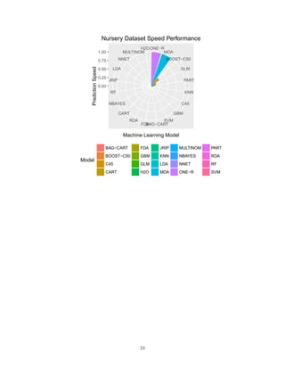
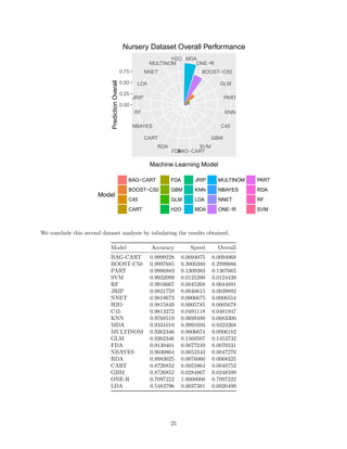

The document benchmarks 20 machine learning models on two datasets to compare their accuracy and speed. On the smaller Car Evaluation dataset, bagged decision trees, random forests and boosted decision trees achieved over 99% accuracy, while neural networks, decision stumps and support vector machines exceeded 95% accuracy. On the larger Nursery dataset, similar models exceeded 99% accuracy, while other models like decision rules and k-nearest neighbors exceeded 95% accuracy. However, models varied significantly in speed depending on the hardware, with decision trees, mixture discriminant analysis and gradient boosting as the fastest on Car Evaluation, and mixture discriminant analysis, one rule and boosted decision trees as the fastest on Nursery. The findings imply the importance of regular benchmarking