Capacity Planning Chapter outline 12.1 Facilities deci.docx

Capacity Planning
Chapter outline
12.1 Facilities decisions
12.2 Facilities strategy
12.3 Sales and operations planning definition
12.4 Cross-functional nature of S&OP
12.5 Planning options
12.6 Basic aggregate planning strategies
12.7 Aggregate planning costs
12.8 Aggregate planning example
12.9 Key points and terms
In this chapter, we discuss capacity decisions related to carrying
out the produc-
tion of goods and services. Firms make capacity planning
decisions that are long
range, medium range, and short range in nature. These decisions
follow naturally
from supply chain decisions that already have been made and
forecasting infor-
mation as an input.

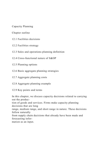
Capacity decisions must be aligned with the operations strategy
of a firm. The
operations strategy provides a road map that is used in making
supply chain deci-
sions to create a network of organizations whose work and
output are used to
satisfy customers' product and service needs. Capacity decisions
are based on
forecasted estimates of future demand. For example, operations
and marketing
collaborate to develop a forecast for demand for resort spa
services before the re-
sort makes capacity planning decisions regarding the
appropriate facility and staff
sizes for the spa.
As was discussed in the previous chapter, long-range decisions
are concerned
with facilities and process selection, which typically extend
about one or more
years into the future. The first part of this chapter describes
facilities decisions and
a strategic approach to making them. In this chapter we also
deal with medium-
range aggregate planning, which extends from six months to a
year or two into the
future. The next chapter discusses short-range capacity
decisions of less than six
months regarding the scheduling of available resources to meet
demand.
Facilities, aggregate planning, and scheduling form a hierarchy
of capacity deci-
sions about the planning of operations extending from long, to
medium, to short
range in nature. First, facility planning decisions are long term

in nature, made to
285
286 Part Four Capacity and Scheduling
FIGURE 12.1
Hierarchy of
capacity decisions.
0
Scheduling
..
6 12
Months
Planning Horizon
18 24
obtain physical capacity that must be planned, developed, and
constructed bef011!
its intended use. Then, aggregate planning determines the
workforce level and p:ro--
duction output level for the medium term within the facility
capacity available
Finally, scheduling consists of short-term decisions that are
constrained by aggregall!
planning and allocates the available capacity by assigning it to
specific activities.
This hierarchy of capacity decisions is shown in Figure 12.1.

Notice that the deci-
sions proceed from the top down and that there are feedback
loops from the b~
tom up. Thus, scheduling decisions often indicate a need for
revised aggrega~
planning, and aggregate planning also may uncover facility
needs.
We define capacity (sometimes referred to as peak capacity) as
the maximum
output that can be produced over a specific period of time, such
as a day, week, or
year. Capacity can be measured in terms of output measures
such as number ot
units produced, tons produced, and number of customers served
over a sp ecified
period. It also can be measured by physical asset availability,
such as the number
of hotel rooms available, or labor availability, for example, the
labor available fO£
consulting or accounting services.
Estimating capacity d ep ends on reasonable assumptions about
facilities, equip-
ment, and workforce availability for one, two, or three shifts as
well as the operat-
ing days per week or per year. If we assume two eight-hour
shifts are available for
five days per week all year, the capacity of a facility is 16 X 5 =
80 hours per week
and 80 X 52 = 4160 hours per year. However, if the facility is
staffed for only one
shift, these capacity estimates must be halved. Facility capacity
is not available un-
less there is a workforce in place to operate it.

Utilization is the relationship between actual output and
capacity and is de-
fined by the following formula:
Actual output
Utilization = C . X 100%
apaCity
The utilization of capacity is a useful measure for estimating
how busy a facility
is or the proportion of total capacity being used . It is almost
never reasonable to
plan for 100 percent utilization since spare (slack) capacity is
needed for planned
and unplanned events. Planned events may include required
maintenance or
equipment replacement, and unpla1med events could be a late
delivery from a
supplier or unexpected demand.
Chapter 12 Capacity Planning 287
-
Operations Leader Bridge Collapse Illustrates Need for
Emergency Capacity
The I-35W Mississippi River bridge near downtown
Mi nneapolis and the University of Minnesota col-
lapsed during the evening rush hour on August 1,
2007. Seventy-five city, county, state, and federal
agencies were involved in the rescue effort. Such cata-
strophic events illustrate the necessity for capacity

availability in emergency services.
The Minneapolis police and fire departments were
among the first responders to the disaster, and while
they generally have excess capacity, utilization of
those services was temporarily pushed to the maxi-
mum. Suburban police and fire units, with their
own available capacity, were brought in to handle
other demands for those services that were unre-
lated to the bridge collapse.
While a majority of injured victims were treated
at Hennepin County Medical Center, nine other area
hospitals also treated victims. Such collaboratio n
among hospital emergency departments is necessary
during large disasters as no single hospital has
enough capacity to absorb these demand spikes.
The excellent working relationships among
agencies that had developed through joint train-
ing, planning, and previous emergency incidents
were cited as one of the primary reasons that re-
sponse and recovery operations went smoothly. As
one rescue leader commented, "We didn't view it
as a Minneapolis incident; it was a city/county/state
incident."
Source: Adapted from information compiled from several
sources, including "I-35W Mississippi River Bridge,"
www.wikipedia.org, 2009.
Utilization rates vary widely by industry and firm. Continuous
flow processes
may have utilization near 100 percent. Facilities with assembly-
line processes may

set planned utilization at 80 percent to allow for flexibility to
meet unexpected
demand. Batch and job shop processes generally have even
lower utiliza tion.
Emergency services such as police, fire, and emergency medical
care often have
fairly low utilization, in part so that they can meet the demands
placed on them
during catastrophic events. The Operations Leader box tells the
story of the Inter-
state 35W bridge collapse in Minneapolis, Minnesota, as an
example of the need
for capacity from a variety of organizations during emergencies.
It is possible in the short term for a firm to operate above 100
percent utilization.
Overtime or an increased work-flow rate can be used in the
short term to meet
highly variable or seasonal demand. Mail and package delivery
services often use
these means to increase work output before major h olidays .
However, firms cannot
sustain this rapid rate of work for more than a short period.
Worker burnout, de-
layed equipment maintenance, and increased costs make it
undesirable to operate
at very high utilization over the medium or long term for most
firms.
In addition to the theoretical peak capacity, there is an effective
capacity that is
obtained by subtracting downtime for maintenance, shift breaks,
schedule
changes, absenteeism, and other activities that d ecrease the
capacity available. The
effective capacity, then, is the amount of capacity that can be

used in planning for
actual facility output over a period of time. To estimate
effective capacity for the
previously described two-shift facility, we must subtract hours
for planned and
unforeseen events.
l
li
I
I
12.1 FACILITIES DECISIONS
"OM: Featuring
St. Alexius
Medical Center,"
Vol. X
Facilities decisions, the longest-term capacity planning
decisions, are of gm1
importance to a firm. These decisions place physical constraints
on the amo.-
that can be produced, and they often require significant capital
investm~
Therefore, facilities decisions involve all organizational
functions and often
made at the highest corporate level, including top management
and the b~
of directors.

Firms must decide whether to expand existing facilities or build
new ones. _
we discuss the facilities strategy below, we will see there are
trade-offs that mm
be considered. Expanding current facilities may provide
location conveniences
current employees but may not be the best location in the long-
run. Alternativell
new facilities can be located near a larger potential workforce
but require duplial-
tion of activities such as maintenance and training.
When construction is required, the lead time for many facilities
decisions r~
from one to five years. The one-year time frame generally
involves buildings -
equipment that can be constructed quickly or leased. The five-
year time frame
volves large and complex facilities such as oil refineries, paper
mills, steel millll
and electricity generating plants.
In facilities decisions, there are five crucial questions:
1. How much capacity is needed?
2. How large should each facility be?
3. When is the capacity needed?
4. Where should the facilities be located?
5. What types of facilities/ capacity are needed?
The questions of how much, how large, when, where, and what
type can be s~
rated conceptually but are often intertwined in practice. As a
result, facilities deci-

sions are exceedingly complex and difficult to analyze.
In the next section, these five types of facilities decisions are
considered in de-
tail. We stress the notion of a facilities strategy, cross-
functional decision ma:king
and the relationship of facilities strategy to business strategy.
12.2 FACILITIES STRATEGY
In Chapter 2 it was noted that a facilities strategy is one of the
major parts of -
operations strategy. Since major facilities decisions affect
competitive success
they need to be considered as part of the total operations
strategy, not simply as
a series of incremental capital-budgeting decisions. Supporting
the operatioot
strategy also applies to other major strategic decisions in
operations regardind
process design, the supply chain, and quality management, as
we have already
noted.
A facilities strategy considers the amount of capacity, the size
of facilities, the
timing of capacity changes, facilities locations, and the types of
facilities needed
for the long run. It must be coordinated with other functional
areas due to the
necessary investments (finance), market sizes that determine the
amount ot
capacity needed (marketing), workforce issues related to
staffing new facilities
(human resources), estimating costs in new facilities
(accounting), and technology

decisions regarding equipment investments (engineering). The
facilities strategy
Amount of
Capacity
FACILITIES STRATEGY.
This Bacardi Rum
factory supplies the
entire North American
market from a single
modern automated
distillery in Puerto
Rico.
needs to be considered in an integrated fashion with these
functional areas and
will be affected by the following factors:
1. Predicted demand. Formulating a facility strategy requires a
forecast of de-
mand; ·techniques for making these forecasts were considered
in the previous chap-
ter. Marketing often is involved in forecasting future demand.
2. Cost of facilities. Cost is driven by the amount of capacity
added at one time,
the timing, and the location of capacity. Accounting and finance
are involved in
estimating future costs and cash flows from facility strategies.
3. Likely behavior of competitors. An expected slow

competitive response may
lead the firm to add capacity to grab the market before
competitors become
strong. In contrast, an expected fast competitive response may
cause the firm to
be more cautious in expanding capacity.
4. Business strategy. The business strategy may dictate that a
company put
more emphasis on cost, service, or flexibility in facilities
choices. For exam-
ple, a business strategy to provide the best service can lead to
facilities with
some excess capacity or several market locations for fast
service. Other busi-
ness strategies can lead to cost minimization or attempts to
maximize future
flexibility.
5. International considerations. As markets and supply chains
continue to be-
come more global in nature, facilities often are located globally.
This involves
not merely chasing cheap labor but locating facilities for the
best strategic ad-
vantage, sometimes to access new markets or to obtain desired
expertise in the
workforce.
One part of a facilities strategy is the amount of capacity
needed. This is deter-
min~d both by forecasted demand and by a strategic decision by
the firm about
how much capacity to provide in relation to expected demand.
This can best be
described by the notion of a capacity cushion, which is defined

as follows:
Capacity cushion = 100% - Utilization
The capacity cushion is the difference between the output that a
firm could achieve
and the real output that it produces to meet demand. Since
capacity utilization
reflects the output required to satisfy demand, a positive
cushion means that there
is more capacity available than is required to satisfy demand.
Zero cushion means
that the average demand equals the capacity available.
Size of
Facilities
The decision regarding a planned amount of cushion is strategic
in na~
The capacity cushion should be planned into capacity decisions,
as the cushiOIIC
will affect service levels as well as the firm's ability to respond
to unexpectel
situations.
Three strategies can be adopted with respect to the amount of
capacity cushi•
1. Large cushion. In this strategy, a large positive capacity
cushion, with ca-
pacity in excess of average demand, is planned. The firm
intentionally has

more capacity than the average demand forecast. This type of
strategy is ap-
propriate when there is an expanding market or when the cost of
buildinfl
and operating capacity is inexpensive relative to the cost of
running out
capacity. Electric utilities adopt this approach, since blackouts
and brown--
outs are generally not acceptable. Firms in growing markets
may adopt a
positive capacity cushion to enable them to capture market
share ahead 01
their competitors. Also, a large cushion can help a firm meet
unpredictabll
customer demand, for example, for new technologies that very
quickly be-
come popular. Firms using a make-to-order process usually have
a signifiJ
cant capacity cushion.
2. Moderate cushion. In this strategy, the firm is more
conservativ e with respect
to capacity. Capacity is built to meet the average forecasted
demand comfort-
ably, with enough excess capacity to satisfy unexpected changes
in demand as
long as the changes are not hugely different from the forecast.
This strategy is
used when the cost (or consequences) of running out is
approximately in bal-
ance with the cost of excess capacity. •
3. Small cushion. In this strategy, a small or nearly zero
capacity cushion is
planned to maximize utilization. This strategy is appropriate
when capacity is

very expensive, relative to stockouts, as in the case of oil
refineries, paper mills,
and other capital-intensive industries. These facilities operate
profitably only at
very high utilization rates between 90 and 100 percent. While
this strategy
tends to maximize short-run earnings, it can be a disadvantage
if competitors
adopt larger capacity cushions. Competitors will be able to meet
any demand in
excess of a firm ' s capacity. Make-to-stock processes are likely
to plan a small
capacity cushion using this strategy.
When planning the capacity cushion, firms assess the
probability of various
levels of demand and then use those estimates to make decisions
about planned
increases or decreases in capacity. For example, suppose a firm
has capacity to
produce 1200 units, SO percent probability of 1000 units of
demand, and SO percent
probability of 800 units of demand. Then average demand is
estimated to be (.S X
1000) + (.S X 800) = 900 units. Producing 900 units results in a
(900 / 1200) X 100%
= 7S% utilization rate. Based on existing capacity, the cushion
is (100% - 7S%) = 2S%.
The solved problems section at the end of the chapter provides
an example of
how to compute the capacity cushion by using probabilities of
demand, existing
levels of capacity, and costs of building capacity. This method
provides a quantita-
tive basis for estimating the amount of capacity cushion that

may be required.
After deciding on the amount of capacity to be provided, a
facilities strategy must
address how large each unit of capacity should be. This is a
question involving
economies of scale, based on the notion that large facilities are
gen erally more
economical because fixed costs can be spread over more units of
production.
FIGURE 12.2
Optimum facility
size.
Timing of
Facility
Decisions
Unit
Cost
Economies of scale
Facility Size (units produced per year)
Economies of scale occur for
two reasons. First, the cost of
building and operating large
production equipment does
not increase linearly with
volume. A machine with

twice the output rate gener-
ally costs less than twice as
much to buy and operate.
Also, in larger facilities the
overhead related to manag-
ers and staff can be spread
over more units of production. As a result, the unit cost of
production falls as facil-
ity size increases when scale economies are present, as shown in
Figure 12.2.
This is a good news-bad news story, for along with economies
of scale come
diseconomies of scale. As a facility gets larger, diseconomies
can occur for several
reasons. First, logistics diseconomies are present. For example,
in a manufacturing
firm, one large facility incurs more transportation costs to
deliver goods to mar-
kets than do two smaller facilities that are closer to their
markets. In a service firm,
a larger facility may require more movement of customers or
materials, for exam-
ple, moving patients around a large hospital or moving mail
through a regional
sorting center. Diseconomies of scale also occur because
coordination costs in-
crease in large facilities. As more layers of staff and
management are added to
manage large facilities, costs can increase faster than output.
Furthermore, costs
related to complexity and confusion rise as more products or
services are added to
a single facility. For these reasons, the curve in Figure 12.2
rises on the right-hand

side due to diseconomies of scale.
As Figure 12.2 indicates, there is a minimum unit cost for a
certain facility size.
This optimal facility size will depend on how high the fixed
costs are and how
rapidly diseconomies of scale occur. As an example, Hewlett-
Packard tends to op-
erate small plants of fewer than 300 workers, with relatively
low fixed costs. This
plant size helps Hewlett-Packard encourage innovation in its
many small product
lines. By contrast, IBM operates very large plants of 5000 to
10,000 workers. IBM
plants tend to be highly automated, and they use a decentralized
management ap-
proach to minimize diseconomies of scale. Each firm seems to
have an optimal
facility size, depending on its cost structure, product/ service
mix, and particular
operations strategy, which may emphasize cost, delivery
flexibility, or service.
Cost is, after all, not the only factor that affects facility size.
Another element of facilities strategy is the timing of capacity
additions. There are
basically two opposite strategies here.
1. Preempt the competition. In this strategy, the firm leads by
building capacity in
advance of the needs· of the market. This strategy provides a
positive capacity
cushion and may actually stimulate the market while at the same
time prevent-
ing competition from coming in for a while. Apple Inc. used
this strategy in the

early days of the personal computer market. Apple built
capacity in advance of
demand and had a lion's share of the market before competitors
moved in.
Apple still uses this strategy today in building massive capacity
and invento-
ries in advance of new product launches for the iPad and
iPhone.
Facility
Location
"Wind Farm
Capacity,"
Vol. XVII
Types of
Facilities
2. Wait and see. In this strategy, the firm waits to
add capacity until demand develops and the
need for more capacity is clear. As a result, the
company lags market demand, using a lower-
·risk strategy. A small or negative capaci
cushion can develop, and a loss of poten ·
market share may result. However, this stra~
egy can be effective because superior market-
ing channels or technology can allow the
follower to capture market share. For examplE;.
in the 1980s, IBM followed the leader (Apple
in the personal computer market but was able

to take away market share because of its supe-
rior brand image, size, and market presence. In
contrast, U.S. automobile companies followed the wait-and-see
strategy, to
their chagrin, for sma ll autos. While U.S. automakers waited to
see how
demand for small cars would develop, Japanese manufacturers
grabbed a dom-
inant position in the U.S. small-car market.
Facility location decisions have become more complex as
globalization has ex-
panded the options for locating capacity and developing new
markets. For example.
Starbucks may choose to build facilities in regions with heavy
coffee drinkers, com-
peting for customers there. Alternatively, it may choose to
locate facilities in regions
where people typically do not consume coffee and attempt to
create demand foc
their product and service. Starbucks's U.S. competitor Caribou
Coffee goes to great
lengths to find facilities locations on the right-hand side of the
road of morning traf-
fic, because customers are more likely to stop frequently when
they can pull over on
the right but are less willing to make cumbersome left-hand
turns in heav y traffic!
Location decisions are made by considering both quantitative
and qualitative fac-
tors. Quantitative factors that affect the location decision may
include return on in-
vestment, net present value, transportation costs, taxes, and lead
times for delivering

goods and services. Qualitative factors can include language
and norms, attitudes
among workers and customers, and proximity to customers,
suppliers, and competi-
tors. Front office services in particular must often locate near
customers for the
customers' convenience, and so this factor may trump most
others in deciding where
to locate new facilities. Examples include banks, grocery stores,
and restaurants.
Firms often compare potential locations b y weighting the
importance of each
factor that is relevant to the decision and then scoring each
potential location on
those factors . Then, multiplying the factor w eight by the
location score allows cal-
culation of a weighted-av erage score for each site. This score
provides insight on
how well each potential site meets the needs of the firm and
may b e used to make
the final facility location decision.
The final element in facility strategy considers the question of
what the firm plans
to accomplish in each facility. There are four different types of
facilities:
1. Product-focused (55 p ercent)
2. Market-focused (30 p ercent)
3. Process-focused (10 p ercent)
4. General-purpose (5 p ercent)

The figures in parentheses indicate the approximate percentages
of companies in
the Fortune 500 using each type of facility.
Product-focused facilities produce one family or type of product
or service,
usually for a large market. An example is the Andersen Window
plant, which pro-
duces various types of windows for the entire United States
from a single product-
focused plant. Product-focused plants often are used when
transportation costs
are low or economies of scale are high. This tends to centralize
facilities into one
location or a few locations. Other examples of product-focused
facilities are large
bank credit card processing operations and auto leasing
companies that process
leases for cars throughout the United States from a single site.
Market-focused facilities are located in the markets they serve.
Many service
facilities fall into this category since services generally cannot
be transported.
Plants that require quick customer response or customized
products or that have
high transportation costs tend to be market focused. For
example, due to the bulky
nature and high shipping costs of mattresses, most production
plants are located
in regional markets. International facilities also tend to be
market focused because
of tariffs, trade barriers, and potential currency fluctuations.

Process-focused facilities have one technology or at most two.
These facilities
frequently produce components or subassemblies that are
supplied to other facili-
ties for further processing. This is common in the auto industry,
in which en-
gine plants and transmission plants feed the final assembly
plants. Process-focused
plants such as oil refineries can make a wide variety of products
within the given
process technology.
Operations Leader Strategic Capacity Planning at BMW '
Mathematical optimization models (e.g., mixed linear
programming) can be helpful in evaluating various ca-
pacity strategies. Given a forecast of demand over the
next several years, the models will determine the min-
imum cost plan for meeting the demand .
An example from BMW helps explain this process.
BMW used a 12-year future planning horizon to rep-
resent the typical development and production life
cycle for new BMW designs. The mathematical
model calculated the supply of finished products
that should be produced by each plant to meet the
forecasts in all global markets.
As a result, the model determined how much of
each product should be produced in each plant over
the next 12 years. All possible locations, amounts,
and types of BMWs were considered by the mathe-
matical model in arriving at the minimum cost plan.
This type of analysis is very helpful in setting overall

capacity strategies for how much, how large, where,
when, and what type. For example, the resulting strat-
egy might be to use distributed production to pro-
duce in each national market the amount sold there
or a more centralized production and export strategy.
Due to the many assumptions made, the models do
not determine the final capacity strategy; however,
they are very helpful in evaluating many different
possibilities.
Source: Fleischmann B., Ferber S. and Henrich P., " Strategic
planning of BMW's Global Production Network," Interfaces,
2006, 36(3): 194-208 ..
li
II
II
II
11
II
II
294 Part Four Capacity arul Scheduling
General-purpose facilities may produce several types of
products and sel'-
vices, using several different processes. For example, general-
purpose facilities a.rr
used to manufacture furniture and to provide consumer banking
and investmenll
services. General-purpose facilities usually offer a great deal of

flexibility in terms
of the mix of products or services that are produced there. They
sometimes are
used by firms that do not have sufficient volume to justify more
than one facili~
Larger firms often focus their faCilities according to product,
market, or procesa
using the focused factory approach described in Chapter 4.
We have shown how the facilities strategy can be developed by
con siderind
questions of capacity, size of facilities, timing, location, and
types of facilities.
Mathematical optimization models can often be helpful in
answering these five
strategic questions as shown in the BMW Operations Leader
box. We now shift
from long-term facilities decisions to medium-term decisions
regarding how
capacity, once built, is used.
12.3 SALES AND OPERATIONS PLANNING DEFINITION
Sales and operations planning (S&OP) is a term used by many
firms to describe the
aggregate planning process. Aggregate planning is the activity
of matching supply
of output with demand over the medium time range. The time
frame is between six
months and two years into the future, or an average of about one
year. The term ag-
gregate implies that the planning is done for a single overall
measure of output or at
most a few aggregated product categories. The aim of S&OP is
to set overall output
levels in the medium-term future in the face of fluctuating or

uncertain demand.
We use a broad definition of S&OP with the following
characteristics:
1. A time horizon of about 12 months, with updating of the plan
on a periodic
basis, perhaps monthly.
2. An aggregate level of demand for one or a few categories of
product. The de-
mand is assumed to be fluctuating, unc~rtain, or seasonal.
3. The possibility of changing both supply and demand
variables.
4. A variety of management objectives, which might include
low inv entories,
good labor relations, low costs, flexibility to increase future
output levels, and
good customer service .
5. Facilities that are considered fixed and cannot be expanded or
reduced.
As a result of S&OP, decisions related to the workforce are
made concerning hir-
ing, laying off, overtime, and subcontracting. Decisions
regarding production out-
put and inventory levels are also made. S&OP is used not only
to plan production
output levels but also to determine the appropriate resource
input mix to use. Since
facilities are assumed to be fixed and cannot be expanded or
contracted, manage-
ment must consider how to use facilities and resources to best

match market
demand.
S&OP can involve plans to influence demand as well as supply.
Factors such as
pricing, advertising, and product mix may be considered in
planning for the me-
dium term. We will discuss these tactics more later in this
chapter.
S&OP generally is done b y product family, that is, a set of
similar products or
services that more or less share a production process, including
the equipment
and workforce needed to produce output. Usually no more than
a few product
Operations Leader S&OP for Household Cleaning Products
Reckitt Benckiser, with £9 billion in sales in 180 coun-
tries, has some of the world's most famous brands, in-
cluding Vanish, Lysol, Calgon, and Airwick. In rapidly
changing retail markets, rapid adjustments in produc-
tion and sales are needed. Because Reckitt has over
500 products in its portfolio, an S&OP system was
needed to coordinate its supply chain.
The S&OP system has been successful, allowing
Reckitt Benckiser to capture 70 percent of grocery
store sales from products that rank first or second in
their categories. Its S&OP team consists of managers

from marketing, sales, production, distribution, and
R&D. Before S&OP, Reckitt Benckiser often used dif-
ferent forecast numbers in different parts of the or-
ganization. It is now able to manage its brands by
"using one set of numbers," says Ariston Banaag.
The team meets regularly to review forecasts and
update plans. The team uses software from Demand
Solution
s to track sales, forecasts, and plans for all its
brands and products.
Source: Adapted from www.demandsolutions.com, 2009
and www.rb.com, 2012.
families are used for S&OP to limit the complexity of the
planning process.
Inconsistencies between supply and demand are resolved by
revising the plan as
conditions change.
S&OP matches supply and demand by using a cross-functional
team ap-
proach. The cross-functional team consisting of marketing,
sales, engineering,

human resources, operations, and finance meets with the general
manager to
agree on the sales forecast, the supply plan, and any steps
needed to modify
supply or demand. During the S&OP process, demand is
decoupled from sup-
ply. For each product family, the cross-functional team must
decide whether to
produce inventory, manage customer lead time, provide
additional capacity
(internal or external), or restrict demand. Once plans to manage
demand and
supply are in balance, however, the current plan may not agree
with previous
financial plans or human resources plans or budgets, which also
may need to be
modified.
The resulting sales and operations plan is updated
approximately monthly, us-
ing a 12-month or longer rolling planning horizon. At its best,
S&OP reduces mis-
alignment among functions by requiring a common plan to be
implemented by all
parties. Strong general manager leadership may be required to

resolve any con-
flicts that arise. Read the Operations Leader box to learn how
S&OP is done for
household cleaning products at Reckitt Benckiser.
Syngenta is a world leader in agribusiness products, with 19,000
employees in
90 countries. The highly seasonal agricultural market is
difficult to forecast and
experiences large demand shifts. Syngenta uses S&OP to create
collaboration
across functions and with its supply chain partners. Managers
across several
countries use the S&OP process and the supporting software to
gain better agree-
ment on forecasts, sales promotions, inv entory levels, sales
plans, and aggregate
production plans. Real-time Web collaboration allows each
business unit to y~
ticipate in the S&OP process to achieve targeted business

goals.1
Since S&OP is a form of aggregate planning, it precedes
detailed schedulioj
which is covered in the next chapter. Scheduling serves to
allocate the capa<4
made available by aggregate planning to specific jobs,
activities, or orders.
12.4 CROSS-FUNCTIONAL NATURE OF S&OP
Aggregate planning for how capacity will be used in the
medium-term future
the primary responsibility of the operations function. However,
it requires cross-
functional coordination and cooperation with all functions in
the firm, includiolll
accounting, finance, human resources, and marketing.
S&OP or aggregate planning is closely related to other business
decisions in-
volving, for example, budgeting, personnel, and marketing. The
relationship
budgeting is particularly strong. Most budgets are based on
assumptions aboul

aggregate output, personnel levels, inventory levels, purchasing
levels, and
forth. An aggregate plan thus should be the basis for initial
budget developm~
and for budget revisions as conditions warrant.
Personnel, or human resource planning, is also greatly affected
by S&OP be-
cause such planning for future production can result in hiring,
lay of, and overti:md
decisions. In service industries, which cannot use inventory as a
buffer againsl
changing demand, aggregate planning is sometimes synonymous
with budgetinG
and personnel planning, particularly in labor-intensive services
that rely heavily
on the workforce to deliver services. •
Marketing must always be closely involved in S&OP because
the future supplJI
of output, and thus customer service, is being determined.
Furthermore, coop era--
tion between marketing and operations is required when both
supply and de-
mand variables are used to determine the best business approach

to aggregate
planning. The next section contains a detailed discussion of the
options available
to modify demand and supply for aggregate planning. This is
followed by the
development of specific strategies that can be used to plan
aggregate output foc
both manufacturing and service industries.
S&OP is not a stand-alone system. It is a key input into the
enterprise resource
planning (ERP) system, which is discussed in Chapter 16. ERP
tracks all d etailed
transactions from orders to shipments to payments, but requires
a high-level ag-
gregate plan for future sales and operations as an input. When
the S&OP p rocess
is used, various scenarios and assumptions can be tested by
simulation to arrive at
an agreed-upon plan that all functions will implement. The ERP
system then ac-
cepts as input the S&OP plan and projects the detailed
transactions (shop orders,
purchase orders, inventories, and payments) that are required to
support the

agreed plan. Figure 12.3 captures these inputs and outputs from
an S&OP process.
In some firms, the S&OP process is broken or missing. Top
management does
not actively support or participate in the process.
Accountability for S&OP is in-
adequate or in conflict across functions. The firm's information
system may not
support S&OP, and so the firm is not able to conduct important
"what if" analy-
sis. Also, S&OP plans may not be executed by all organizational
functions as has
been agreed. Therefore, to be successful, the S&OP system may
require changes
in the organization, reporting and accountability, and the
information systems.
1 Herrin (2004).
FIGURE 12.3
lelationship of
S&OP with other

lanctions.
Accounting
-Cost analysis
Finance
Operations
- Forecast
- Inventory levels
-Capacity
-Current orders
- Investment
Marketing
-Forecast
-Sales plan
/
S&OP ")

, Process 1
1 "-.... ///
" ........ ---- .,.
Human Resources
- Personnel
planning
12.5 PLANNING OPTIONS
Operations and marketing must work closely to plan for
matching supply and
demand over the medium-term time frame. They do this during
aggregate plan-
ning when they coordinate their decisions to develop enough
demand for prod-
ucts and services without overshooting available facility
capacity.
The S&OP process can be clarified by a discussion of the
various decision op-
tions available. These include two categories of decisions: (1)

those modifying de-
mand and (2) those modifying supply.
Demand management entails modifying or influencing demand
in several
ways:
1. Pricing. Differential pricing often is used to reduce peak
demand or to build up
demand in off-peak periods. Some examples are matinee movie
prices, off-
season hotel rates, factory discounts for early- or late-season
purchases, and
off-peak specials at restaurants. The purpose of these pricing
schemes is to level
demand through the day, week, month, or year.
2. Advertising and promotion. These methods are used to
stimulate or in some
cases smooth out demand. Advertising can be timed to promote
demand dur-
ing slack periods and shift demand from peak periods to slack
times. For ex-
ample, ski resorts advertise to lengthen their season and turkey
growers

advertise to stimulate demand outside the peak holiday seasons.
3. Backlogs or reservations. In some cases, demand is
influenced by asking cus-
tomers to wait for their orders (backlog) or by reserving
capacity in advance
(reservations). Generally, this has the effect of shifting demand
from peak
"Service Design
at Hotel Monaco,"
Vol. IX
periods to periods with slack capacity. However, the waiting
time may resu
a loss of business. This loss can be tolerated when the aim is to
maximize~
although most operations are extremely reluctant to tum away
customers.

4. Development of complementary offerings. Firms with highly
seasonal
mands may try to develop products that have countercyclic
seasonal trends.
example, Taro produces both lawn mowers and snow blowers,
seasonally ~
plementary products that can share production facilities. In fast-
food reslil
rants, breakfast has been added in many cases to utilize
previously idle capaq
The service industries, using all the mechanisms described
above, have .:
much further than most of their manufacturing counterparts in
influencing
mand. Because they are unable to inventory their output-their
services---til
use these mechanisms to improve their utilization of fixed
facility capacity.
Supply management includes a variety of factors that can be
used to increase
decrease supply through aggregate planning. These factors
include the followinll

1. Hiring and laying off employees. Some firms will do almost
anything ~
reducing the size of the workforce through layoffs. Other
companies routinll
increase and decrease the workforce as demand changes. These
practices, "'
vary widely by firm and industry, affect not only costs but also
labor relatiollll
productivity, and worker morale. As a result, company hiring
and layoff p~
tices may be restricted by union contracts or company policies.
These effedll
must be factored into decisions about whether to change the size
of the w0111
force to match demand more closely.
2. Using overtime and undertime. Overtime sometimes is used
for short-
medium-range labor adjustments in lieu of hiring and layoffs,
especially if
change in demand is considered temporary. Overtime labor
usually costs 1
percent of regular time, with double time on weekends and
holidays. BecaU!IIIII

of its high cost, managers are sometimes reluctant to use
overtime. F~
more, workers may be reluctant to work more than 20 percent
weekly overt:ioll
for an extended p eriod. Undertime refers to planned
underutilization of ~
workforce rather than layoffs, perhaps by using a shortened
workweek. Undefll
time, in the form of furloughs, was common in many industries,
includillllll
manufacturing, education, and government, during the
recessionary months
2008-2009.
3. Using part-time or temporary labor. In some cases, it is
possible to hire pan<
time or temporary employees to meet peak or seasonal demand.
This option
particularly attractive when part-time employees are paid
significantly less
wages and benefits. Unions frequently frown on the use of part-
time employe~!~
because those employees often do not pay union dues and may
weaken uni~
influence. Temporary labor is more likely to be used to satisfy

seasonal or shod-·
to medium-term demand. Part-time labor and temporary labor
are used exten-
sively in many service operations, such as restaurants,
hospitals, su permarkel!i
and department stores. Temporary labor is also common in
agriculture-relatel
industries.
4. Carrying inventory. In manufacturing firms, inventory can be
used as a buffer-
between supply and demand. Inventories for later use can be
built up during
periods of slack demand. Inventory thus decouples supply from
demand in
manufacturing operations, allowing for smoother operations
with more even
use of capacity throughout a time period. Inventory is a way to
store expended
capacity and labor for future consumption. This option is

generally not avail-
able for service operations; this results in greater challenges for
service indus-
tries in matching supply and demand.
5. Subcontracting. Subcontracting is the outsourcing of work
(either manufactur-
ing or service activities) to other firms. This option can be very
effective for in-
creasing or decreasing supply. The subcontractor may supply
the entire product
or service or only some of the components. For example, a
manufacturer of toys
may utilize subcontractors to make plastic parts during periods
of high de-
mand. Service operations may subcontract secretarial
assistance, call center op-
erations, catering services, or facilities during peak periods.
6. Cooperative arrangements. These arrangements are similar to
subcontracting in
that other sources of supply are used, but cooperative
arrangements often in-
volve partner firms that are typically competitors. The firms
choose to share their

capacity, thus preventing either firm from building capacity that
would be used
only during brief periods. Examples include electric utilities
that link their capac-
ity through power-sharing networks, hospitals that send patients
to other hospi-
tals either for certain specialized services or during demand
peaks, and hotels or
airlines that shift customers among one another when they are
fully booked.
In considering all these options, it is clear that S&OP and the
aggregate plan-
ning problem are extremely broad and affect most parts of the
firm. The decisions
that are made are therefore strategic and cross-functional,
reflecting all the firm's
objectives. If aggregate planning is considered narrowly,
inappropriate decisions
result and suboptimization may occur. Some of the multiple
trade-offs that should
be considered are customer service level (through back orders
or lost demand),
inventory levels, stability of the labor force, and costs. The
conflicting objectives

and trade-offs among these elements sometimes are combined
into a single cost
function. A method for evaluating costs is described later in this
chapter.
12.6 BASIC AGGREGATE PlANNING STRATEGIES
When demand slumped, the Parker Hannifin plastic parts
manufacturing plant in
Spartanburg, South Carolina, kept its workforce but reduced
work hours where
Using a level strategy often results in holding inventory
during low demand periods.
possible. In contrast, the investment firm Goldman
Sachs laid off 10 percent of its workforce in late
2008 and another 10 percent in early 2009. In this
section, we discuss the aggregate planning strate-
gies used in each of these instances and explain
how firms decide which strategy is best for them.
Two basic planning strategies can be used, as
well as combinations of them, to meet medium-
term aggregate demand. One strategy is to main-

tain a level workforce; the other is to chase demand
with the workforce.
With a perfectly level strategy, the size of the
workforce and the rate of regular-time output
are constant. Any variations in demand must
be absorbed by using inventories, overtime,
temporary workers, subcontracting, cooperative
Operations Leader Travelers' Level Strategy Meets Demand
Variation
Travelers offers a wide variety of insurance products
and services, covering customers in more than 90
countries. It sells insurance for auto owners, renters,
home owners,
TRAVELER 5 'f , ~;a~~~~~n~:s:~
example of a

service firm that uses a level strategy to manage its
workforce and capacity.
Before Hurricane Ike slammed the Texas coast in
September 2008, Travelers claims employees from
around the United States were moving toward the af-
fected areas so that they would be immediately avail-
able to serve affected customers. Even before the
storm made landfall, teams of trained and equipped
claims professionals were ready. The company's Na-
tional Catastrophe Response Center had plans in place
to quickly deploy thousands of cross-trained employ-
ees from other regions to help customers rather
than, as is customary in the industry, relying on out-
side contractors.
Travelers uses a level strategy, with workers from
many regions pitching in during large-scale disasters
and workers being diverted to training and catch-up
activities during slow times when it might appear to
be overstaffed. The strategy seems to pay off in
terms of maintaining high levels of customer service
during a peak demand period. Travelers was able to
contact most of its Hurricane Ike-affected customers

within 48 hours of their reporting a claim and to in-
spect, provide payment, and close the majority of
claims within 30 days.
Source: Adapted from annual report, www.travelers.com,
2009.
arrangements, or any of the demand-influencing options
discussed above. The
level strategy essentially holds the regular workforce at a fixed
number, and so
the rate of workforce output is fixed over the aggregate
planning period .
However, a firm using a level strategy can respond to
fluctuations in demand
by using the demand and supply planning options discussed in
the previous
section.
With the chase strategy, the size of the workforce is changed to
meet, or chase,
demand. With this strategy, it is not necessary to carry
inventory or use the de-
mand and supply planning options available for aggregate
planning; the work-

force absorbs all the changes in demand. The chase strategy
generally results in a
fair amount of hiring and laying off of workers as demand is
chased.
These two strategies are extremes; one strategy makes no
change in the work-
force, and the other varies the workforce directly with demand
changes. In prac-
tice, many firms use a combination of these two strategies. Read
the Operations
Leader box to see how Travelers Insurance successfully uses a
level strategy even
though demand for its service can vary significantly.
Consider, for example, a brokerage firm that utilizes both
strategies. The data
processing department maintains the capacity to process 17,000
transactions per
day, far in excess of the average load of 12,000. This capacity
allows the depart-
ment to keep a level workforce of programmers, systems
analysts, and computer
operators even though capacity exceeds demand on many days.
Because of the

skilled workforce, the high capital investment, and the
difficulty and expense of
hiring replacements, the data processing department chooses to
follow a level
strategy.
Meanwhile, in the cashiering department, a chase strategy is
used. As the
transaction level varies, part-time workers, hiring, and layoffs
are used. This de-
partment is very labor-intensive, with high worker turnover and
low skill levels
TABLE 12.1
,.Comparison of
Chase and Level
Strategies
Level of labor skill required
Job discretion
Compensation rate
Training required per employee

Labor turnover
Hire-layoff costs per employee
Amount of supervision required
Type of budgeting and forecasting required
Chase Strategy
Low
Low
Low
Low
High
Low
High
Short run
Level Strategy
High
High
High
High
Low

High
Low
Long run
required . The manager of the department commented that the
high turnover
rate is an advantage, facilitating the reduction of the workforce
in periods of low
demand.
From this scenario, we see that the characteristics of the
operation seem to influ-
ence the type of strategy followed . This observation can be
generalized to the fac-
tors shown in Table 12.1. While the chase strategy may be more
appropriate for
low-skilled labor and routine jobs, the level strategy seems
better for highly skilled
labor and complex jobs.
These strategies can be compared in terms of their costs to
provide insight into
the better choice, depending on the particular situation a firm
faces. The relevant
factors in this decision are represented by their cost, allowing

us to develop mod-
els to compare the two strategies, as described in the next
section.
12.7 AGGREGATE PLANNING COSTS
.
Most aggregate planning methods include a plan that minimizes
costs. These
methods assume that demand is given (based on forecasts) but
varies over time;
therefore, strategies for modifying demand are not considered.
If both demand
and supply are modified simultaneously, it may be more
appropriate to develop a
model to maximize profit rather than minimize costs, since
demand changes affect
revenues along with costs.
When demand is given, the following costs should be included:
1. Hiring and layoff costs. Hiring costs consist of the recruiting,
screening, and
training costs required to bring a new employee up to full
productive skill. For

some jobs, this cost may be only a few hundred dollars; for
more highly skilled
jobs, it may be thousands of dollars. Layoff costs include
employee benefits,
severance pay, and other associated costs. This cost also may
range from a few
hundred to several thousand dollars per worker. When an entire
shift of work-
ers is hired or laid off, a shift cost must be accounted for.
2. Overtime and undertime costs. Overtime costs consist of
regular wages plus
an overtime premium, typically an additional 50 to 100 percent.
Undertime
costs reflect the use of employees at less than full productivity.
3. Inventory-carrying costs. Inventory-carrying costs are
associated with main-
taining goods in inventory, including the cost of capital, the
variable cost of stor-
age, obsolescence, and deterioration. These costs often are
expressed as a
percentage of the dollar value of inventory, ranging from 15 to
35 percent per year.

This cost can be thought of as an interest charge assessed
against the dolW
value of inventory held in stock. Thus, if the carrying cost is 20
percent and
each unit costs $10 to produce, it will cost $2 to carry one unit
in invent0111
for a year.
4. Subcontracting costs. The cost of subcontracting is the price
paid to anot:hfti
firm to produce the units. Subcontracting costs can be either
greater or less t:ru.
the cost of producing units in-house. .
5. Part-time labor costs. Due to differences in benefits and
hourly rates, the ced
of part-time or temporary labor is often less than that of regular
labor. Al-
though part-time workers often receive no benefits, a maximum
percentagtt
of part-time labor may be specified by operational

considerations or by uni«mm
contract. Otherwise, there might be a tendency to use all part-
time or tempo-~
rary labor. However, the regular labor force is generally
essential for opera-
tions continuity as well as to utilize and train part-time and
temporaiJI
workers effectively.
6. Cost of stockout or back order. The cost of taking a back
order or the cost ot
a stockout should reflect the effect of reduced customer service.
This cost is
extremely difficult to estimate, but it should capture the loss of
custom~
goodwill, the loss of profit from the order, and the possible loss
of future
sales.
Some or all of these costs may be relevant in any aggregate
planning problem.
The applicable costs can be used to "price out" alternative
decisions and strate-
gies. In the example below, the total costs related to three
alternative strategies are

estimated. When this type of analysis is conducted o~ a
spreadsheet, a very large
number of alternative strategies can be considered.
12.8 AGGREGATE PLANNING EXAMPLE
FIGURE 12.4
Hefty Beer
Company- demand
forecast.
The Hefty Beer Company is constructing an aggregate plan for
the next 12 months.
Although several types of beers are brewed at the Hefty plant
and several con-
tainer sizes are bottled, management has decided to use gallons
of beer as the ag-
gregate measure of capacity.
The demand for beer over the next 12 months is forecast to
follow the p attern
shown in Figure 12.4. Notice that demand peaks during the
summer months and
is decidedly lower in the winter.

700
600
8
0
3 500
"' c:<
0
~ 400
0
300
200
I ~
v
,/ -/ ~
lL
v
J F M A M J p A S 0 N D

Month
The management of the Hefty brewery would like to consider
three aggregate
plans:
1. Level workforce. Use inventory to meet peak demands.
2. Level workforce plus overtime. Use 20 percent overtime
along with inventory
in June, July, and August to meet peak demands.
3. Chase strategy. Hire and lay off workers each month as
necessary to meet
demand.
To evaluate these strategies, management has collected the
following cost and
resource data:
• Assume the starting workforce is 40 workers. Each worker can

produce 10,000
gallons of beer per month on regular time. On overtime, the
same production
rate is assumed, but overtime can be used for only three months
during the
year.
• Each worker is paid $2000 per month on regular time.
Overtime is paid at 150
percent of regular time. A maximum of 20 percent overtime can
be used.
• Hiring a worker costs $1000, including screening, paperwork,
and training
costs. Laying off a worker costs $2000, including all severance
and benefit costs.
• For inventory valuation purposes, beer costs $2 a gallon to
produce. The cost of
carrying inventory is estimated to be 3 percent per month (or 6
cents per gallon
of beer per month).
• Assume the starting inventory is 50,000 gallons. The desired
ending inventory

a year from now is also 50,000 gallons. All forecast demand
must be met; no
stockouts are allowed.
The next task is to evaluate each of the three strategies in terms
of the costs
given. The first step in this process is to construct spreadsheets
like those shown
in Tables 12.2 through 12.4, which show all the relevant costs:
regular workforce,
overtime, hiring/layoff, and inventory. Notice that
subcontracting, part-time
labor, and back orders/ stockouts have not been used as
variables in this case.
To evaluate the level strategy, we calculate the size of the
workforce required to
meet the demand and inventory goals. Since ending and
beginning inventories are
assumed to be equal, the workforce must be just large enough to
meet total de-
mand during the year. When the monthly demands from Figure
12.4 are summed,
the annual demand is 5,400,000 gallons. Since each worker can
produce 10,000(12)

= 120,000 gallons per year, a level workforce of 5,400,000--:-
120,000 = 45 workers
is needed to meet the total demand. This means that five new
workers must be
hired. The inventories for each month and the resulting costs
have been calculated
in Table 12.2.
Consider the calculations for January. With 45 regular workers
entered at the
top of the table, 450,000 gallons of beer can be produced, since
each worker pro-
duces 10,000 gallons in a month. The production exceeds the
sales forecast by
150,000 (450,000- 300,000) gallons, which is added to the
beginning inventory of
50,000 gallons to yield an inventory level of 200,000 gallons at
the end of January.
Next the costs in Table 12.2 are calculated as follows: Regular
time costs are
$90,000 in January (45 workers X $2000 each). There is no
overtime cost, but 5
workers have been hired, since the starting workforce level was
40 workers. The

cost of hiring these five workers is $5000. Finally, it cost 6
cents to carry a gallon of
beer in inventory for a month, and Hefty is carrying 200,000
gallons at the end of
w
0
""'
TABLE 12.2
Aggregate Planning Cos ts-Strategy 1, Level Workforce*
Jan. Feb. Mar. Apr. May June July Aug.
Resources
Regular workers 45 45 45 45 45 4 5 45 45
Overtime(%) 0 0 0 0 0 0 0 0
Units produced 450 450 450 450 450 450 450 450

Sales fo recast 300 300 350 4 00 450 500 6 50 600
Invent ory (end of month) 200 350 450 500 500 4 50 250 100
Costs
Regular time $90.0 $90.0 $90.0 $90.0 $90.0 $90.0 $90.0 $90.0
Overtime 0.0 0.0 0.0 0.0 0.0 0.0 0.0 0 .0
Hire/layoff 5.0 0 .0 0.0 0 .0 0.0 0.0 0.0 0.0
Inventory carrying 12.0 2 1.0 27.0 30.0 30.0 27.0 15.0 6.0
Total cost $ 107.0 $ 111.0 $11 7.0 $120.0 $ 120.0 $1l 7.0
$105.0 $96.0
• All costs are expressed in thousands of dollars. All production
and inventory figures are in thousands of gallons. Starting
inventory is 50,000 gallons.
Sept. Oct. Nov. Dec. Total
4 5 45 45 45

0 0 0 0
450 450 450 4 50 5400
4 75 475 450 450 5400
75 50 50 50
$90 .0 $90.0 $90.0 $90.0 $1080 .0
0.0 0.0 0.0 0.0 0.0
0.0 0.0 0 .0 0.0 5.0
4 .5 3.0 3.0 3.0 18 1.5
$94.5 $93.0 $93.0 $93.0 $ 1266.5
w
0
U1
TABLE. 12.3

Aggregate Planning Costs-Strategy 2, Level with Overtime*
Jan. Feb. Mar. Apr. May June July Aug. Sept.
Resources
Regular workers 43 43 43 43 43 43 43 43 43
Overtime(%) 0 0 0 0 0 20 20 20 0
Units produced 430 430 430 430 430 516 516 516 430
Sales forecast 300 300 350 400 450 500 650 600 475
Inventory (end of month) 180 310 390 420 400 416 282 198 153
~
Costs
Regular time $86.0 $86.0 $86.0 $86.0 $86.0 $86.0 $86.0 $86 .0
$86.0
Overtime 0.0 0.0 0.0 0.0 0.0 25.8 25.8 25 .8 0.0
Hire/layoff 3.0 0.0 0.0 0.0 0.0 0.0 0.0 0.0 0.0

Inventory carrying 10.8 18.6 23.4 25.2 24.0 25.0 16.9 11.9 9.2
Total cost $99.8 $104.6 $109.4 $111.2 $110.0 $136 .8 $128.7
$123 .7 $95 .2
'All costs are expressed in thousands of dollars. All production
and inventory figures are in thousands of gallons. Starting
TABLE 12.4
Aggregate Planning Costs-Strategy 3, Chase Demand*
Jan. Feb. Mar. Apr. May June July Aug. Sept.
Resources
Regular workers 30 30 35 40 45 50 65 60 48
Overtime (%) 0 0 0 0 0 0 0 0 0
Units produced 300 300 350 400 450 500 650 600 480
Sales forecast 300 300 350 400 450 500 650 600 4 75

Inventory (end of month) 50 50 50 50 50 50 50 50 55
Costs
Regular time $60 .0 $60.0 $70.0 $80.0 $90.0 $100.0 $130.0
$120.0 $96.0
Overtime 0.0 0.0 0.0 0 .0 0.0 0.0 0.0 0 .0 0.0
Hire/layoff 20.0 0.0 5.0 5.0 5.0 5.0 15.0 10 .0 24.0
Inventory carrying 3.0 3 .0 3.0 3 .0 3.0 3.0 3.0 3.0 3.3
Total cost $83.0 $63 .0 $78.0 $88.0 $198.0 $108.0 $148.0
$133.0 $1 23.3
• All costs are expressed in thousands of dollars. All production
and inventory figures are in thousands of gallon s. Starting
Oct. Nov. Dec. Total
43 43 43
0 0 0

430 430 430 5418
475 450 450 5400
108 88 68
$86.0 $86 .0 $86 .0 $1032.0
0.0 0.0 0.0 77.4
0.0 0.0 0.0 3 .0
6.5 5.3 4 .1 180.8
$92 .5 $91. 3 $90.1 $ 1293 .2
Oct. Nov. Dec. Total
47 4 5 45
0 0 0
470 450 450 5400

475 450 4 50 5400
50 50 50
$94.0 $90.0 $90.0 $1080 .0
0.0 0 .0 0.0 0.0
2.0 4.0 0.0 95 .0
3 .0 3 .0 3.0 36.3
$99.0 $97.0 $93. 0 $ 1211.3
TABLE 12.5
Cost Summary
Strategy 1-Level
Regular-time payroll
Hire/layoff
Inventory carrying

Total
Strategy 2-Level with overtime
Hire/layoff
Overtime
Inventory carrying
Total
Strategy 3-C hase
Hire/layoff
Inventory carrying
Total
$1 ,080,000
5,000
181,500
$1,266,500
$1 ,032, 000

3,000
77,400
180 ,800
$1,293,2 00
$1 ,080,000
95,000
36,300
$1,211 ,300
the month, which costs $12,000.2 These costs total $107,000 for
January. The calcu-
lations are continued for each month and then summed for ti;.e
year to yield the
total cost of $1,266,500 for the level strategy.
The second strategy, level workforce plus overtime, is a bit
more complicated. If
X is the workforce size for option 2, we must have
9(10,000X) + 3[(1.2)(10,000X) ] = 5,400,000 gallons

For nine months Hefty will produce 10,000X gallons per month,
and for three
months it will produce 120 percent of 10,000X, including
overtime. When the above
equation is solved for X, we find X = 43 workers. In Table 12.3
we have calculated
the inventories and resulting costs for this option.
The third strategy, the chase strategy, varies the workforce each
month by hir-
ing and laying off workers to meet monthly demand exactly.
When this strategy is
used, a constant level of 50,000 gallons in inventory is
maintained as the minimum
inventory level, as shown in Table 12.4.
The annual costs of the three strategies are summarized in Table
12.5. On the ba-
sis of the given costs and assumptions, the chase strategy is the
lowest-cost strategy.
However, cost is not the only consideration. For example, the
chase strategy requires
building from a minimum workforce of 30 to a peak of 65
workers, and then layoffs
are used to reduce the number back to 45 workers. Will the

labor climate permit this
amount of hiring and laying off each year, or will this lea d to
unionization and po-
tentially higher labor costs? Maybe a two-shift policy or the use
of part-time or tem-
porary workers should be considered for peak demand portions
of the year. These
alternatives, along with others, should be considered in
attempting to evaluate and
possibly improve on the chase strategy, as we have done in the
chapter supplement
We have shown how to compare costs in a very simple case of
aggregate planning
by using three potential strategies. Advanced methods have
been developed to con-
sider many more strategies and more complex aggregate
planning problems. These
methods, which can be quite complex, include linear
programming, simulation, and
various decision rules.
2 For convenience, we use the end-of-month inventory to
calculate inventory-carrying costs rather tha n
the averag e monthly invento ry.

12.9 KEY POINTS AND TERMS
The following key points are discussed in the chapter:
• Facilities decisions consider the amount of capacity, the size
of units, the timing
of capacity changes, facility location, and the types of facilities
needed. These
are long-range decisions in the hierarchy of capacity decisions.
Facilities deci-
sions are crucial because they determine the future availability
of output and
require the organization's scarce capital.
• A facility strategy should be implemented rather than a series
of incremental
facility decisions. A facilities strategy answers the questions of
how much, how
large, where, when, and what type.

• The amount of capacity planned should be based on the
desired risk of
meeting forecast demand. The capacity cushion is a decision
that firms
must consider, determining whether they will use a large
cushion and not
run short of capacity or a small cushion with the possibility of a
capacity
shortage.
• When it is timing capacity expansion, a firm can choose to
preempt the com-
petition by building capacity sooner or wait and see how much
capacity is
needed.
• Both economies and diseconomies of scale should be
considered in setting an
optimum facility size. Facility location is determined by
considering relevant
factors in this decision and then weighing contrasting factors
against one an-
other. The type of facility selected is focused on product,
market, process, or
general-purpose needs.

• Facilities. decisions often are made by the chief executive and
the board of direc-
tors . Because these d ecisions are strategic in nature, they
require the input of all
functional areas in the firm .
• Sales and operations planning (S&OP), or aggregate planning,
serves as the link
between facilities decisions and scheduling. S&OP decisions set
output levels
for the medium time range. As a result, decisions regarding
workforce size,
subcontracting, hiring, and inventory levels are also made.
These decisions
must fit within the facilities capacity available and are
constrained by the re-
sources av ailable.
• Aggregate planning is concerned with matching supply and
demand over the
medium time range. There are many options for managing
supply and demand.
Because human resources, capital, and demand are affected, all
functions must

be involved in aggregate planning decisions.
• Supply factors that can be changed by aggregate planning are
hiring, layoffs,
overtime, under time, inventory, subcontracting, part-time
labor, and coopera-
tive arrangements. Factors that influence demand are pricing,
promotion, back-
log or reservations, and complementary products.
• There are two basic .strategies for adjusting supply: the chase
strategy and
the level strategy. Firms can also use a combination of these
two main
strategies. A choice of strategy can be analyzed by estimating
the total cost
of each of the av ailable strategies. Factors, other than costs, to
consider are
cu stomer serv ice levels, d em and shifts, the labor force, and
forecasting
accuracy.

Key Terms
STUDENT
INTERNET
EXERCISES
~ •
Hierarchy of capacity
decisions 285
Capacity 286
Utilization 286
Effective capacity 287
Facilities decisions 288
Facilities strategy 288
Capacity cushion 289
Economies of scale 290
Diseconomies of scale 291
1. Course site:
Preempt the
competition 291

Wait-and-see
strategy 292
Product-focused
facilities 293
Market-focused
facilities 293
Process-focused
facilities 293
http://www.uoguelph.ca/-dsparlin!aggregat.htm
General-purpose
facilities 293
Sales and operations
planning 294
Aggregate planning 294
Demand
management 297

Supply management 298
Level strategy 299
Chase strategy 300
Read this synopsis of aggregate planning from Professor Dave
Sparling's course
in Canada.
2. Spreadsheet example from Georgia Southern University
http://et.nmsu.edu/-etti/winter97/computers/spreadsheet.html
Work through the details of this example to gain a deeper
understanding of ag-
gregate planning.
3. Sales and Operations Planning
http://www.supplychain.com
Read about S&OP on this site and come to class prepared for a
discussion.
4. Demand

Capacity Planning Chapter outline 12.1 Facilities deci.docx

Capacity Planning Chapter outline 12.1 Facilities deci.docx

Recommended

Recommended

More Related Content

Similar to Capacity Planning Chapter outline 12.1 Facilities deci.docx

Similar to Capacity Planning Chapter outline 12.1 Facilities deci.docx (20)

More from humphrieskalyn

More from humphrieskalyn (20)

Recently uploaded

Recently uploaded (20)

Capacity Planning Chapter outline 12.1 Facilities deci.docx