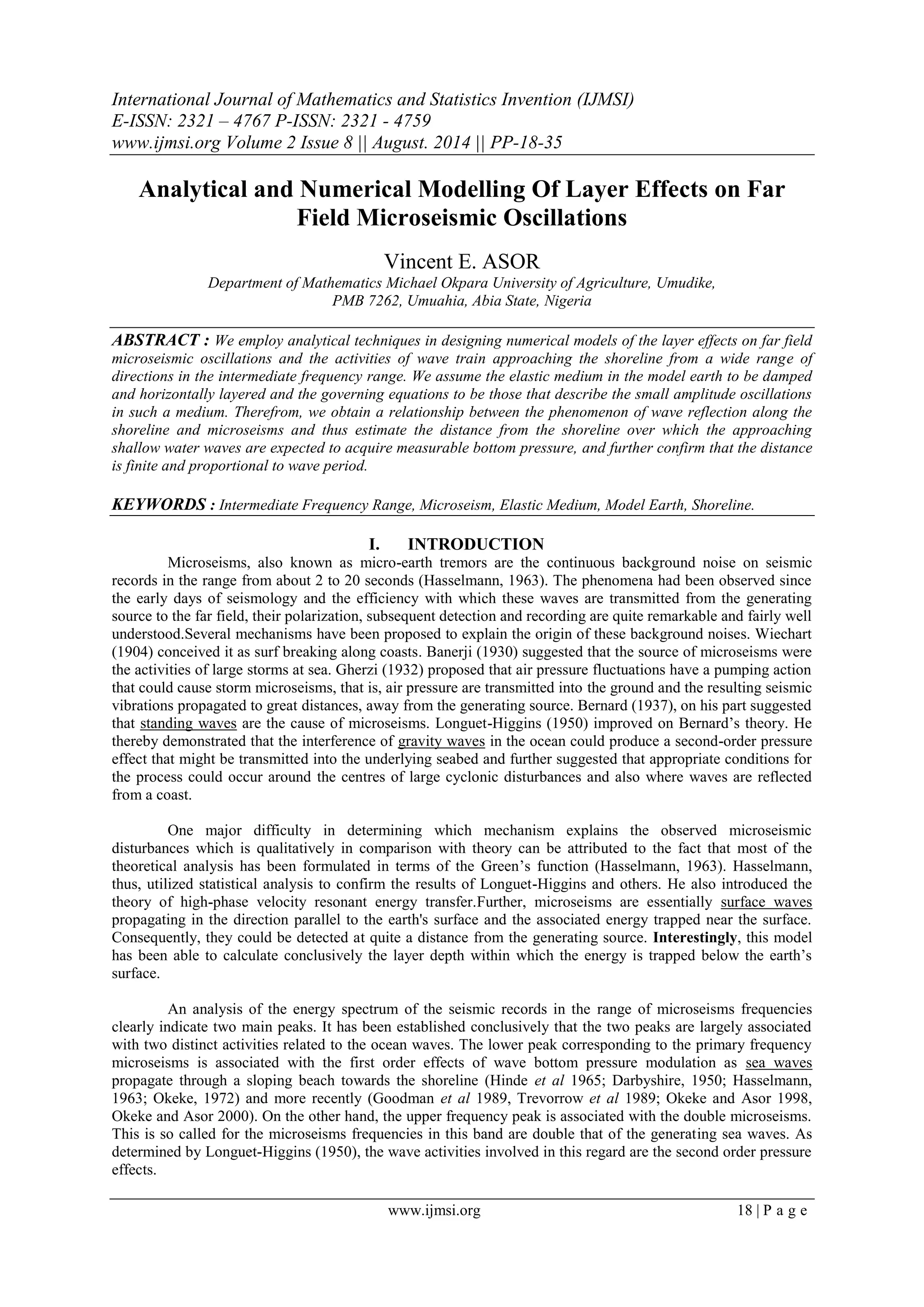
International Journal of Mathematics and Statistics Invention (IJMSI) is an international journal intended for professionals and researchers in all fields of computer science and electronics. IJMSI publishes research articles and reviews within the whole field Mathematics and Statistics, new teaching methods, assessment, validation and the impact of new technologies and it will continue to provide information on the latest trends and developments in this ever-expanding subject. The publications of papers are selected through double peer reviewed to ensure originality, relevance, and readability. The articles published in our journal can be accessed online.
Wave-Current Interaction Model on an Exponential Profileijceronline
We develop a model that approximates the exponential depth, which exhibits the behavior of linear depth particularly in the surf zone. The main effect of the present exponential depth is found in the shoaling zone, where the depth remains finite. The basic description and the outcome is essentially rip currents where in the surf zone the wave behavior is the same as found in the linear depth case. In the shoaling zone the present exponential depth exhibits the hypergeometric functions.
M6.0 2004 Parkfield Earthquake : Seismic AttenuationAli Osman Öncel
HRSN isimli kuyu içi sismik istasyonlar kullanılarak, San Andreas fayı boyunca meydana gelen büyük depremler öncesi sismik azalımın varlığının olup olmadığı araştırılıyor.
Review of Analysis of Retaining Wall Under Static and Seismic Loadingijsrd.com
This paper presents a comparison of the various methods of analysis of retaining wallsunder seismic loads, which is considered to be very complex.As the soil-structure interaction during the earthquake is very complex, the most commonly used methods for the seismic design of retaining walls are the Pseudo static method, Seed and Whitman method and Mononobe and Okabe method. The retaining wall analysis includes determining the factor of safety for overturning, and sliding as well as the resultant location of the forces, which must be within the middle- third of the footing,. A concrete retaining wall is considered with a certain height and base width, and then analyzed for the static case as well as the earthquake loading condition. Based on this study, it is found that factor of safety obtained by Seed & Whitman method (1970) is lowest as compared to others methods.
A high-resolution 3D seismic velocity model of the 2010 Mw 8.8 Maule, Chile e...Stephen Hicks
Knowledge of the spatial distribution of seismic properties within an earthquake rupture zone is essential to our understanding of rupture mechanics. Following the Maule earthquake, there was an international collaborative effort to deploy a dense network of seismic instruments in order to record the aftershock sequence; this means a large dataset is available to perform seismic velocity tomography in the area of the rupture zone. Since most co-seismic slip occurred in the offshore region, it is important to interpret the velocity structure of the marine forearc and the underlying oceanic crust. However, since many aftershocks are located offshore, and thus outside of the land network, both the offshore velocity structure and the location of these aftershocks are inherently poorly resolved. During the period July - December 2010, The National Taiwan Ocean University and The University of Liverpool each deployed ocean-bottom seismometer (OBS) networks in the northern and southern ends of the rupture zone, respectively, comprising a total of 43 stations. We use a catalogue of ~500 seismic events recorded at both land and OBS stations, containing ~60000 hand-picked P- and S-wave travel-times. We use a staggered 1D inversion scheme, which initially incorporates a separate velocity model for the marine forearc in order to form better hypocentral locations for the offshore events. Based on previous estimates for slab geometry, we find that the location of offshore seismicity is more tightly constrained along and above the interface. Taking these improved locations into account, we then re-invert for a new 1D model with station corrections. We present a 3D local earthquake tomography model based on manually-picked arrival times. The incorporation of OBS picks into the inversion elucidates better both the up-dip geometry of the subducting plate and the structure of the marine forearc. Beneath the low vp marine forearc (vp < 6.0 km/s), at depths of 7-15 km, we infer the presence of a high velocity structure (vp > 7.0 km/s); the upper interface of which dips at 10-15°, interpreted as the top of the downgoing oceanic crust. These first-order features are in accordance with results from previous active source studies in the region. We continue to analyse the nature and geometry of velocity anomalies along and around the megathrust, and their relation to rupture models and aftershock distribution.
Unraveling Earthquake Dynamics Through Extreme-Scale Multi-Physics Simulations
ALICE GABRIEL (LUDWIG MAXIMILIAN UNIVERSITY OF MUNICH, GERMANY)
Earthquakes are highly non-linear multiscale problems, encapsulating geometry and rheology of faults within the Earth’s crust torn apart by propagating shear fracture and emanating seismic wave radiation.
This talk will focus on using physics-based scenarios, modern numerical methods and hardware specific optimizations to shed light on the dynamics, and severity, of earthquake behaviour. It will present the largest-scale dynamic earthquake rupture simulation to date, which models the 2004 Sumatra-Andaman event - an unexpected subduction zone earthquake which generated a rupture of over 1,500 km in length within the ocean floor followed by a series of devastating tsunamis.
The core components of the simulation software will be described, highlighting the benefits of strong collaborations between domain and computational scientists. Lastly, future directions in coupling the short-term elastodynamics phenomena to long-term tectonics and tsunami generation will be discussed.
https://pasc18.pasc-conference.org/program/keynote-presentations/
The performance of soil slope during an earthquake is generally analyzed by three different approaches which are pseudo-static methods, Newmark’s Sliding Block method and numerical techniques. In pseudo-static approach, the effects of an earthquake are represented by constant vertical (kv) and horizontal (kh) seismic acceleration coefficients and the factor of safety is evaluated by using limit equilibrium or limit analysis or finite element method of analysis. Newmark’s sliding block method evaluates the expected displacement of slope subjected to any ground motion obtained from the integration of the equation of motion for a rigid block sliding in an inclined plane. Numerical methods determine the expected displacements obtained from the stress – strain relationship of a soil mass. In this paper the stability of a model soil slope, comprising of an embankment with two canal bunds at the top, at different stages of construction, i.e. only embankment, embankment with empty canal bunds and embankment with canal bunds filled with water, with different foundation soils in different seismic zones have been analyzed and results have been plotted in the form of variation of factor of safety with horizontal seismic acceleration coefficient (kh). The critical case has been further analyzed under dynamic conditions. Dynamic analyses have been carried out by plotting the response spectrum curve and selecting 2001 Bhuj earthquake motion as the typical ground motion.
International Journal of Engineering and Science Invention (IJESI) is an international journal intended for professionals and researchers in all fields of computer science and electronics. IJESI publishes research articles and reviews within the whole field Engineering Science and Technology, new teaching methods, assessment, validation and the impact of new technologies and it will continue to provide information on the latest trends and developments in this ever-expanding subject. The publications of papers are selected through double peer reviewed to ensure originality, relevance, and readability. The articles published in our journal can be accessed online.
Marmara ve İstanbul için ayrı ayrı 2 senaryo yapılmış. Coulomb Stress etkisi önemli ölçüde deprem olasılığını yükseltiyor. Özellikle, KAFZ boyunca meydana gelen depremlerin yüzey kırıklarının Dünya'da ki benzer büyük depremlerin yüzey kırıklarından oldukça farklı ve büyük.
Seismic Microzonation Study in Tabriz Metropolitan City for Earthquake Risk M...IJERA Editor
Azerbaijan is the site of convergent plate collisions along the Alpine-Himalayan active mountain belt. Brittle
faults in the Azerbaijan area are mostly Cenozoic in or younger. The data presented demonstrate clearly that
geological structures are commonly repeated at all scales from outcrop to regional. Several regional earthquakes
have been strongly felt and caused damages in and around Tabriz during history. Urban seismic risk is
increasing with population growth and encroachment of vulnerable built in environment into areas susceptible
seismic hazard. Seismic -hazard assessment an estimate of ground motion at the site of interest, taking into
account instrumental and historical earthquake records, information on tectonics, geology, and
attenuation characteristics of seismic waves Tabriz is important industrial city of Iran. It has a very high
population density about 2.000000 people in area just 90 km2. The main objective of the Tabriz seismic
instrumentation and microzonation study was to carry out and propose new building in Tabriz and suburbs in
order to apply these criteria its development programs and determine the potential for damage to
existing constructions during earthquake motions, and finally earthquake risk mitigation assessment.
Modeling the Frictional Effect on the Rip Current on a Linear Depth Profileijceronline
We develop an analytical theory for the interaction between waves and currents induced by breaking waves on a depth profiles. Here we examine the effect of friction on the rip currents and so are not particularly concerned with frictionally determined rip currents. The near shore is characterized by the presence of breaking waves, and so we develop equations to be used outside the surf zone, based on small-amplitude wave theory, and another set of equations to be used inside the surf zone, based on an empirical representation of breaking waves. Suitable matching conditions are applied at the boundary between the offshore shoaling zone and the near shore surf zone. Both sets of equation are obtained by averaging the basic equations over the wave phase. Thus the qualitative solution constructed is a free vortex defined in both shoaling and surf zone where in the surf zone the free vortex is perturbed by a long shore component.
International Journal of Computational Engineering Research(IJCER)ijceronline
International Journal of Computational Engineering Research(IJCER) is an intentional online Journal in English monthly publishing journal. This Journal publish original research work that contributes significantly to further the scientific knowledge in engineering and Technology.
International Journal of Mathematics and Statistics Invention (IJMSI) is an international journal intended for professionals and researchers in all fields of computer science and electronics. IJMSI publishes research articles and reviews within the whole field Mathematics and Statistics, new teaching methods, assessment, validation and the impact of new technologies and it will continue to provide information on the latest trends and developments in this ever-expanding subject. The publications of papers are selected through double peer reviewed to ensure originality, relevance, and readability. The articles published in our journal can be accessed online.
Crustal Anisotropy in the Martian Lowlands From Surface WavesSérgio Sacani
The largest seismic event ever recorded on Mars, with a moment magnitude of 4.7 ± 0.2, is
the first event to produce both Love and Rayleigh wave signals. We measured their group velocity dispersion
between about 15 and 40 s period and found that no isotropic depth-dependent velocity model could explain
the two types of waves wave simultaneously, likely indicating the presence of seismic anisotropy. Inversions
of Love and Rayleigh waves yielded velocity models with horizontally polarized shear waves traveling faster
than vertically polarized shear waves in the top 10–25 km. We discuss the possible origins of this signal,
including the preferred orientation of anisotropic crystals due to shear deformation, alignment of cracks, layered
intrusions due to an impact, horizontal layering due to the presence of a large-scale sediment layer on top of the
crust, and alternation of sedimentation and basalt layers deposits due to large volcanic eruptions.
International Journal of Computational Engineering Research(IJCER)ijceronline
International Journal of Computational Engineering Research(IJCER) is an intentional online Journal in English monthly publishing journal. This Journal publish original research work that contributes significantly to further the scientific knowledge in engineering and Technology
Different Martian Crustal Seismic Velocities across the Dichotomy Boundary fr...Sérgio Sacani
Article This article is protected by copyright. All rights reserved.
Abstract
We have observed both minor-arc (R1) and major-arc (R2) Rayleigh waves for the largest marsquake (magnitude
of 4.7 ± 0.2) ever recorded. Along the R1 path (in the lowlands), inversion results show that a simple, two-layer
model with an interface located at 21 - 29 km and an upper crustal shear-wave velocity of 3.05 - 3.17 km/s can fit the
group velocity measurements. Along the R2 path, observations can be explained by upper crustal thickness models
constrained from gravity data and upper crustal shear-wave velocities of 2.61 - 3.27 km/s and 3.28 - 3.52 km/s in the
lowlands and highlands, respectively. The shear-wave velocity being faster in the highlands than in the lowlands
indicates the possible existence of sedimentary rocks, and relatively higher porosity in the lowlands.
First Observation of the Earth’s Permanent FreeOscillation s on Ocean Bottom ...Sérgio Sacani
The Earth’s hum is the permanent free oscillations of the Earth recorded in the absence ofearthquakes, at periods above 30 s. We present the first observations of its fundamental spheroidaleigenmodes on broadband ocean bottom seismometers (OBSs) in the Indian Ocean. At the ocean bottom,the effects of ocean infragravity waves (compliance) and seafloor currents (tilt) overshadow the hum. In ourexperiment, data are also affected by electronic glitches. We remove these signals from the seismic traceby subtracting average glitch signals; performing a linear regression; and using frequency-dependentresponse functions between pressure, horizontal, and vertical seismic components. This reduces the longperiod noise on the OBS to the level of a good land station. Finally, by windowing the autocorrelation toinclude only the direct arrival, the first and second orbits around the Earth, and by calculating its Fouriertransform, we clearly observe the eigenmodes at the ocean bottom.
Estimation of Poisson’s Ratio of Ozizza Subsurface Layersiosrjce
A geophysical survey aimed at determining the Poisson’s ratio of subsurface earth materials have
been carried out. Knowledge of the Poisson’s ratio of materials is important since it gives information about the
quality of such materials with respect to construction works. The study area is Ozizza (lat. 5.80
-5.90N; long.
7.80
-7.90E) situated within the Afikpo sedimentary basin in south - eastern Nigeria. The geophysical method
employed was the seismic refraction method and both P - and S - waves were utilized. The major equipment
used was a MOD.S79 seismograph and its accessories including P- and S- wave sources and detectors. The
result shows that the P- waves delineated three layers with average velocities of 420m/s, 1745m/s and 2620m/s
for the first, second and third layers from the earth’s surface respectively whereas the S-waves revealed only
two layers with average velocities of 310 m/s and 1100 m/s for the first and second layers accordingly. The
result indicates that the first and second layers of Ozizza (probably made up of sandy clay and sand with gravel
have Poisson’s ratio of 0.22 and 0.28 respectively.
Welcome to the first live UiPath Community Day Dubai! Join us for this unique occasion to meet our local and global UiPath Community and leaders. You will get a full view of the MEA region's automation landscape and the AI Powered automation technology capabilities of UiPath. Also, hosted by our local partners Marc Ellis, you will enjoy a half-day packed with industry insights and automation peers networking.
📕 Curious on our agenda? Wait no more!
10:00 Welcome note - UiPath Community in Dubai
Lovely Sinha, UiPath Community Chapter Leader, UiPath MVPx3, Hyper-automation Consultant, First Abu Dhabi Bank
10:20 A UiPath cross-region MEA overview
Ashraf El Zarka, VP and Managing Director MEA, UiPath
10:35: Customer Success Journey
Deepthi Deepak, Head of Intelligent Automation CoE, First Abu Dhabi Bank
11:15 The UiPath approach to GenAI with our three principles: improve accuracy, supercharge productivity, and automate more
Boris Krumrey, Global VP, Automation Innovation, UiPath
12:15 To discover how Marc Ellis leverages tech-driven solutions in recruitment and managed services.
Brendan Lingam, Director of Sales and Business Development, Marc Ellis
Generative AI Deep Dive: Advancing from Proof of Concept to ProductionAggregage
Join Maher Hanafi, VP of Engineering at Betterworks, in this new session where he'll share a practical framework to transform Gen AI prototypes into impactful products! He'll delve into the complexities of data collection and management, model selection and optimization, and ensuring security, scalability, and responsible use.
Pushing the limits of ePRTC: 100ns holdover for 100 daysAdtran
At WSTS 2024, Alon Stern explored the topic of parametric holdover and explained how recent research findings can be implemented in real-world PNT networks to achieve 100 nanoseconds of accuracy for up to 100 days.
GDG Cloud Southlake #33: Boule & Rebala: Effective AppSec in SDLC using Deplo...James Anderson
Effective Application Security in Software Delivery lifecycle using Deployment Firewall and DBOM
The modern software delivery process (or the CI/CD process) includes many tools, distributed teams, open-source code, and cloud platforms. Constant focus on speed to release software to market, along with the traditional slow and manual security checks has caused gaps in continuous security as an important piece in the software supply chain. Today organizations feel more susceptible to external and internal cyber threats due to the vast attack surface in their applications supply chain and the lack of end-to-end governance and risk management.
The software team must secure its software delivery process to avoid vulnerability and security breaches. This needs to be achieved with existing tool chains and without extensive rework of the delivery processes. This talk will present strategies and techniques for providing visibility into the true risk of the existing vulnerabilities, preventing the introduction of security issues in the software, resolving vulnerabilities in production environments quickly, and capturing the deployment bill of materials (DBOM).
Speakers:
Bob Boule
Robert Boule is a technology enthusiast with PASSION for technology and making things work along with a knack for helping others understand how things work. He comes with around 20 years of solution engineering experience in application security, software continuous delivery, and SaaS platforms. He is known for his dynamic presentations in CI/CD and application security integrated in software delivery lifecycle.
Gopinath Rebala
Gopinath Rebala is the CTO of OpsMx, where he has overall responsibility for the machine learning and data processing architectures for Secure Software Delivery. Gopi also has a strong connection with our customers, leading design and architecture for strategic implementations. Gopi is a frequent speaker and well-known leader in continuous delivery and integrating security into software delivery.
Why You Should Replace Windows 11 with Nitrux Linux 3.5.0 for enhanced perfor...SOFTTECHHUB
The choice of an operating system plays a pivotal role in shaping our computing experience. For decades, Microsoft's Windows has dominated the market, offering a familiar and widely adopted platform for personal and professional use. However, as technological advancements continue to push the boundaries of innovation, alternative operating systems have emerged, challenging the status quo and offering users a fresh perspective on computing.
One such alternative that has garnered significant attention and acclaim is Nitrux Linux 3.5.0, a sleek, powerful, and user-friendly Linux distribution that promises to redefine the way we interact with our devices. With its focus on performance, security, and customization, Nitrux Linux presents a compelling case for those seeking to break free from the constraints of proprietary software and embrace the freedom and flexibility of open-source computing.
Epistemic Interaction - tuning interfaces to provide information for AI supportAlan Dix
Paper presented at SYNERGY workshop at AVI 2024, Genoa, Italy. 3rd June 2024
https://alandix.com/academic/papers/synergy2024-epistemic/
As machine learning integrates deeper into human-computer interactions, the concept of epistemic interaction emerges, aiming to refine these interactions to enhance system adaptability. This approach encourages minor, intentional adjustments in user behaviour to enrich the data available for system learning. This paper introduces epistemic interaction within the context of human-system communication, illustrating how deliberate interaction design can improve system understanding and adaptation. Through concrete examples, we demonstrate the potential of epistemic interaction to significantly advance human-computer interaction by leveraging intuitive human communication strategies to inform system design and functionality, offering a novel pathway for enriching user-system engagements.
The Art of the Pitch: WordPress Relationships and SalesLaura Byrne
Clients don’t know what they don’t know. What web solutions are right for them? How does WordPress come into the picture? How do you make sure you understand scope and timeline? What do you do if sometime changes?
All these questions and more will be explored as we talk about matching clients’ needs with what your agency offers without pulling teeth or pulling your hair out. Practical tips, and strategies for successful relationship building that leads to closing the deal.
Accelerate your Kubernetes clusters with Varnish CachingThijs Feryn
A presentation about the usage and availability of Varnish on Kubernetes. This talk explores the capabilities of Varnish caching and shows how to use the Varnish Helm chart to deploy it to Kubernetes.
This presentation was delivered at K8SUG Singapore. See https://feryn.eu/presentations/accelerate-your-kubernetes-clusters-with-varnish-caching-k8sug-singapore-28-2024 for more details.
Climate Impact of Software Testing at Nordic Testing DaysKari Kakkonen
My slides at Nordic Testing Days 6.6.2024
Climate impact / sustainability of software testing discussed on the talk. ICT and testing must carry their part of global responsibility to help with the climat warming. We can minimize the carbon footprint but we can also have a carbon handprint, a positive impact on the climate. Quality characteristics can be added with sustainability, and then measured continuously. Test environments can be used less, and in smaller scale and on demand. Test techniques can be used in optimizing or minimizing number of tests. Test automation can be used to speed up testing.
Removing Uninteresting Bytes in Software FuzzingAftab Hussain
Imagine a world where software fuzzing, the process of mutating bytes in test seeds to uncover hidden and erroneous program behaviors, becomes faster and more effective. A lot depends on the initial seeds, which can significantly dictate the trajectory of a fuzzing campaign, particularly in terms of how long it takes to uncover interesting behaviour in your code. We introduce DIAR, a technique designed to speedup fuzzing campaigns by pinpointing and eliminating those uninteresting bytes in the seeds. Picture this: instead of wasting valuable resources on meaningless mutations in large, bloated seeds, DIAR removes the unnecessary bytes, streamlining the entire process.
In this work, we equipped AFL, a popular fuzzer, with DIAR and examined two critical Linux libraries -- Libxml's xmllint, a tool for parsing xml documents, and Binutil's readelf, an essential debugging and security analysis command-line tool used to display detailed information about ELF (Executable and Linkable Format). Our preliminary results show that AFL+DIAR does not only discover new paths more quickly but also achieves higher coverage overall. This work thus showcases how starting with lean and optimized seeds can lead to faster, more comprehensive fuzzing campaigns -- and DIAR helps you find such seeds.
- These are slides of the talk given at IEEE International Conference on Software Testing Verification and Validation Workshop, ICSTW 2022.
PHP Frameworks: I want to break free (IPC Berlin 2024)Ralf Eggert
In this presentation, we examine the challenges and limitations of relying too heavily on PHP frameworks in web development. We discuss the history of PHP and its frameworks to understand how this dependence has evolved. The focus will be on providing concrete tips and strategies to reduce reliance on these frameworks, based on real-world examples and practical considerations. The goal is to equip developers with the skills and knowledge to create more flexible and future-proof web applications. We'll explore the importance of maintaining autonomy in a rapidly changing tech landscape and how to make informed decisions in PHP development.
This talk is aimed at encouraging a more independent approach to using PHP frameworks, moving towards a more flexible and future-proof approach to PHP development.
PHP Frameworks: I want to break free (IPC Berlin 2024)
C028018035
1. International Journal of Mathematics and Statistics Invention (IJMSI)
E-ISSN: 2321 – 4767 P-ISSN: 2321 - 4759
www.ijmsi.org Volume 2 Issue 8 || August. 2014 || PP-18-35
www.ijmsi.org 18 | P a g e
Analytical and Numerical Modelling Of Layer Effects on Far Field Microseismic Oscillations Vincent E. ASOR Department of Mathematics Michael Okpara University of Agriculture, Umudike, PMB 7262, Umuahia, Abia State, Nigeria ABSTRACT : We employ analytical techniques in designing numerical models of the layer effects on far field microseismic oscillations and the activities of wave train approaching the shoreline from a wide range of directions in the intermediate frequency range. We assume the elastic medium in the model earth to be damped and horizontally layered and the governing equations to be those that describe the small amplitude oscillations in such a medium. Therefrom, we obtain a relationship between the phenomenon of wave reflection along the shoreline and microseisms and thus estimate the distance from the shoreline over which the approaching shallow water waves are expected to acquire measurable bottom pressure, and further confirm that the distance is finite and proportional to wave period. KEYWORDS : Intermediate Frequency Range, Microseism, Elastic Medium, Model Earth, Shoreline.
I. INTRODUCTION
Microseisms, also known as micro-earth tremors are the continuous background noise on seismic records in the range from about 2 to 20 seconds (Hasselmann, 1963). The phenomena had been observed since the early days of seismology and the efficiency with which these waves are transmitted from the generating source to the far field, their polarization, subsequent detection and recording are quite remarkable and fairly well understood.Several mechanisms have been proposed to explain the origin of these background noises. Wiechart (1904) conceived it as surf breaking along coasts. Banerji (1930) suggested that the source of microseisms were the activities of large storms at sea. Gherzi (1932) proposed that air pressure fluctuations have a pumping action that could cause storm microseisms, that is, air pressure are transmitted into the ground and the resulting seismic vibrations propagated to great distances, away from the generating source. Bernard (1937), on his part suggested that standing waves are the cause of microseisms. Longuet-Higgins (1950) improved on Bernard’s theory. He thereby demonstrated that the interference of gravity waves in the ocean could produce a second-order pressure effect that might be transmitted into the underlying seabed and further suggested that appropriate conditions for the process could occur around the centres of large cyclonic disturbances and also where waves are reflected from a coast. One major difficulty in determining which mechanism explains the observed microseismic disturbances which is qualitatively in comparison with theory can be attributed to the fact that most of the theoretical analysis has been formulated in terms of the Green’s function (Hasselmann, 1963). Hasselmann, thus, utilized statistical analysis to confirm the results of Longuet-Higgins and others. He also introduced the theory of high-phase velocity resonant energy transfer.Further, microseisms are essentially surface waves propagating in the direction parallel to the earth's surface and the associated energy trapped near the surface. Consequently, they could be detected at quite a distance from the generating source. Interestingly, this model has been able to calculate conclusively the layer depth within which the energy is trapped below the earth’s surface. An analysis of the energy spectrum of the seismic records in the range of microseisms frequencies clearly indicate two main peaks. It has been established conclusively that the two peaks are largely associated with two distinct activities related to the ocean waves. The lower peak corresponding to the primary frequency microseisms is associated with the first order effects of wave bottom pressure modulation as sea waves propagate through a sloping beach towards the shoreline (Hinde et al 1965; Darbyshire, 1950; Hasselmann, 1963; Okeke, 1972) and more recently (Goodman et al 1989, Trevorrow et al 1989; Okeke and Asor 1998, Okeke and Asor 2000). On the other hand, the upper frequency peak is associated with the double microseisms. This is so called for the microseisms frequencies in this band are double that of the generating sea waves. As determined by Longuet-Higgins (1950), the wave activities involved in this regard are the second order pressure effects.
2. Analytical And Numerical Modelling Of Layer...
www.ijmsi.org 19 | P a g e
These are energized through the nonlinear interactions among progressive sea waves moving in
opposite directions. The phenomena are not affected by the depth of the water layer. Consequently, they are
effective generating mechanism both in deep and shallow water areas. In our studies, we have included the
activities of the generating water waves approaching the shoreline from a wide range of directions. Also, our
elastic medium which is the model Earth is damped and horizontally layered with the governing equations being
those that describe the small amplitude oscillations in such a medium. Our study also introduces a damping term
in the governing equations representing the effect of the material inelasticity which we shall assume to be slight.
This enables us to adopt the model due to Darbyshire and Okeke (1969) in which the damping term in the
equation of motion is assumed to be proportional to the time rate of the change of material displacement
components in the first normal incident theory. Previous calculations based on this model were quite close to the
measurements of seismic events in the far field.
Further, there are a number of interesting and innovative publications on the evolution of the
microseisms in the seafloor. Recent achievements in this area of geophysics owe a lot to the work of Yamamoto
et al (1977, 1978) and recently, Trevorrow et al (1988, 1989). Information acquired therefrom had been
effectively used in the study of such areas as the structural depth profile below the seabed. We have extended
this analysis with identical calculations to the far field microseisms activities. Generally, previous investigators
based their models on the theory of the homogenous earth without incorporating the effect of earth’s layering in
the numerical calculations. In this regard therefore, we have analysed the effects of earth’s layering on far field
micro-earth tremors while extending the normal incident theory of Darbyshire and Okeke (1969) to two
dimensions.
II. GOVERNING EQUATIONS AND THEIR SPECIFICATIONS
The x-axis and y-axis are taken as perpendicular and along the shoreline respectively. The z-axis points
vertically downwards with z=0 as the earth’s surface, t>0 is the time with t=0 giving the onset of the
geophysical activities involved in our subsequent studies.The behaviour of an isotropic solid is completely
specified if and are given ( is the modulus of elasticity, is the Lamé’s constant). In particular, defines
the strength of the layered elastic solid, hence, the most important parameter in our present investigation. s is
the density of solid which, in the case of horizontally stratified elastic half-space, will be a function of z. Finally,
the displacement components of the elastic half-space in response to the seismic events are U, V, W in the x, y
and z directions respectively.
With these specifications, the governing equations are:
( ) 0 2
2
2
U
t x
U
s (2.1)
( ) 0 2
2
2
V
t y
V
s (2.2)
( ) 0 2
2
2
W
t z
W
s (2.3)
where
2
2
2
2
2
2
2 ,
z x y z
W
y
V
x
U
Differentiate both sides of equations (2.1) with respect to x, (2.2) with respect to y and (2.3) with respect to z
and add, then,
2 2
2
2
t
(2.4)
where defines the wave of compression which moves with the speed where
s
( 2 ) 2
.
Further, differentiate both sides of equations (2.2) with respect to z and (2.3) with respect to y, then subtract, we
obtain
x
x
t
2 2
2
2
(2.5)
3. Analytical And Numerical Modelling Of Layer...
www.ijmsi.org 20 | P a g e
z
V
y
W
x
(2.6)
In the same way we obtain
y
y
t
2 2
2
2
(2.6a)
z
U
x
V
y
(2.6b)
and z
z
t
2 2
2
2
(2.6c)
y
U
x
W
z
(2.6d)
The vector
( x , y , z ) (2.6e)
gives the wave of rotation in the elastic solid which moves with speed where
s
2
(2.6f)
It is to be noted however that, for surface waves, we assume the motion to be uniform with respect to the y-axis.
We then introduce two scalar potentials and for the displacements of the elastic solid. Thus, we have,
x z
U
,
z x
V
(2.6g)
Using the above equation, with
2
2
2
2
2
2 x z
, then
2
2
z
W
x
U
(2.7)
2
2
x
W
z
U
y (2.8)
Equations (2.7) and (2.8) indicate that the scalar potentials and are respectively related to the waves of
compression and rotation. Thus, introducing (2.7) and (2.8) into (2.4) and (2.6) respectively, we obtain the wave
equations in the form
2
2
2
2
2
t
(2.9)
2
2
2
2
2
t
(2.10)
Details of the above equations are found in Bullen & Bolt (1985), Burridge (1976).
III. GRAVITY WAVES AND GROUND MOVEMENTS
A gravity wave is an oscillation caused by the displacement of an air parcel which is restored to its
initial position by gravity. The lifting force is buoyancy, while the restoring force is gravity. In this
consideration, we introduce a damping term into the governing equations to represent the effect of material
inelasticity which we shall assume to be small since the oscillations take place near the Earth’s surface
(0<z<100m) and the variations in the elastic parameters are slight.
Introducing and in equation (2.1) with (2.2) and using the same notations therein, we have the following
system of equations:
4. Analytical And Numerical Modelling Of Layer...
www.ijmsi.org 21 | P a g e
x z z x z t x z
P k e s
ik x ct
2
2
2
2
2
2
2
( ) ( ) 2 (3.1)
2 0
2
2
2
2 2
x z x z t z x
s
(3.2)
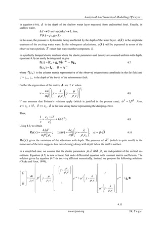
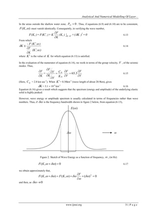
In (3.1), the term on the left hand side is the generating pressure field of the water waves; P(k) being the
amplitude spectrum of the bottom pressure. The wave number k and the phase speed c are such as to match
those of the seismic trapped modes below the seabed. Hence, k and c will refer to both the generating water
waves and the seismic response of the elastic half-space in the subsequent discussion.
The solutions of equations (3.1) and (3.2) are expressible in the form:
(x, z, t) Aexp[ik(rz x ct)] (3.3)
(x, z, t) Bexp[ik(sz x ct)] (3.4)
where A and B do not depend on space and time.
1
1
2
2
2
2
2
2
c
s
c
r
(3.5)
The effect of damping term introduced in equations (3.1) and (3.2) is to make k and c complex with non-zero
immaginary part. Thus, k k ik 0 and c c ic 0 but, k k 0 and c c 0
On the earth's surface and in the far field, the waveforms are free, hence, the equations (3.1) to (3.5) gives:
[ ( 1) ] [2 ] 0 2 2 2 A s c B s sc (3.6)
[2 ] [ (1 ) ] 0 2 2 2 A r cs B s c (3.7)
Equations (3.6) and (3.7) above are consistent if
( ) (2 ) [ (1 ) ] 0 2 2 2 2 2 f c c rs s c (3.8)
Eliminating r and s in equation (3.8) using (3.5), then,
( ) (2 ) [( ) 1] [ (2 ) ] 0 4
2
2
2 4 1 2 2 c
c c
f c c
(3.9)
With as the medium’s Poisson's constant, we introduce the following notations:
c
k
1 1 and
2( )
,
2 2
1 2
Thus, equation (3.9) gives
(2 ) ( 1) [ (2 ) ] 0 4
1 1
2
1
2
1
4
1 k k k k (3.10)
Rearranging equation (3.10) as an equation in 1 k ,
24 ] 16 (1 2 ) 16 (1 ) 0
( 1)}] 4 [ (2 1) 2 (4 3)] [8 (3 2 )
( ) ( ) 4 ( 2 ) [8 {6 (4 1)
2
1
4
1 1
2 2
1
2 2
2
1
2 4
1
2
1
2 2
1
3 2
1
2
1
2
2
1
4 4 2 2
1
2
1
5 2 2
1
2 4
1
6 4
1 1
k
k k
f k k k k
(3.11)
In an undamped elastic medium ( 0 ), equation (3.11) reduces to the usual equation for the non-dispersive
Rayleigh waves in elastic solid. In this case, the equation reduces to a cubic equation in
2
1 k which has been
thoroughly analysed (Bullen and Bolt, 1985) to obtain the propagational properties of the surface waves for a
5. Analytical And Numerical Modelling Of Layer...
www.ijmsi.org 22 | P a g e
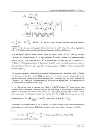
range of values of . Equation (3.11) therefore, exemplifies the case of material dispersion in which 1 k and
are coupled. So, attenuation term induces material dispersion into an otherwise non-dispersive Rayleigh surface
waves in the elastic material (Okeke and Asor, 2000).
Equation (3.11) is a sixth order equation and so has six roots that are complex conjugate in the 1 k -plane. It
cannot be reduced to a cubic equation because it contains terms involving odd powers of 1 k . However,
quantitative analysis (Okeke and Asor, 2000), suggests that, (0) 16 (1 ) 0 2
1
2 f since 0 1 1
for surface waves. f (1) 0 because
[ (2 4 ) ( 4 )] 16 (1 ) (4 ) 0 2 3
1
2 2 2
1
3 for each term in the bracket is
negative since 1 1 and
4
because, is small. Thus, there is a root of 3.11 in [0,1] 1 k .
For f (1) , we have
0
59 3
16
10
4 6 (8 1) 4 (4 1) (2 1)
3
32
2 2 31
1
2
8
4 7
2
1
2 4
1
2 3
1
4 3 2 2
for
4
and introducing the realistic values of and 1 .
Therefore, there is at least a root of equation (3.11) between 0 1 k and 1 1 k . In brief, there are roots of
equation (3.11) in the circle of unit radius 1 1 k and none on the circumference 1 1 k .
In the studies involving surface waves, 1 1 k , so, the interest is roots of equation (3.11) in the circle. To do
this, sequence ( ), 1,2,3,4,5 1 f k m m of Sturm’s function (Kurosh, 1980) are computed from the equation
(3.11).
We now let ( ) ( ) 0 1 1 f k f k as in equation (3.11); ( ) 1 f k m be taken as the first derivative of
( ), 1,2,3,4,5 1 1 f k n n . Further, let c(0) be the number assigned to the changes of sign in these sequences
when 0 1 k . Attach an identical meaning to c(1) when 1 1 k . In this consideration, it is deduced that the
difference c(0) c(1) in 0 1 1 k depends on the assigned values of . From symmetry, identical
conclusion applies for the difference c(0) c(1) in 1 0 1 k .
Consequently, if
40
0
2
1
, then c(0) c(1) 1 and there is only one real root in each of the interval
1 0 1 k and 0 1 1 k . In this case, propagating elastic waves are undamped. With regards to the
Sturm’s sequence, all the leading coefficients are positive. However, for higher values of in the range
40 4
2
1
, the leading coefficients for m 2 and m 3 in the Sturm’s sequence are negative and
c(0) c(1) 2 . Thus, in 1 1 k , there are four complex conjugate roots, one in each of the four quadrants of
the 1 k -plane. Consequently, this analysis convincingly proves that seismic waves in an elastic solid are
effectively damped if the attenuation coefficient inherent in the solid exceeds the value
40
2
1
. Thus, it is
concluded that, the effectiveness of the damping of elastic vibrations in elastic solid is a function of the strength
of the solid material. Put differently, the more rigid a solid is, the greater is the damping of elastic vibrations
6. Analytical And Numerical Modelling Of Layer...
www.ijmsi.org 23 | P a g e
passing through it. In practice, the upper limit of
4
is never attained. In particular, the complex root in the first
quadrant of k -plane for which Re( ) 0, Im( ) 0 1 1 k k corresponds to the observed damped seismic
vibration.
We now apply this result to the microseismic signals recorded on land below which is made of fairly hard rock.
With this earth’s structure, the phase speed, 0 c , of the seismic signal ranges from
1 1.1 sec km to
1 1.8 sec km . Using the value 0.8 0 c , the corresponding value of is between
1 0.021 sec km to
1 0.04 sec km . This range of values of is between
40
2
1
and
4
suggesting strongly that the microseismic
signals propagating from the source to the recording station in the far field are damped appreciably.
The variation of this range of values of with depth is shown in Asor (2000). The uniformity of this range with
depth is apparent. The calculations cover the case of the horizontally stratified earth for which the elastic
parameters and density are functions of the z -co-ordinates only. Further, the calculations are confined to the
shallow earth’s layer below the surface.
IV. THE FREQUENCY SPECTRAL AMPLITUDE COMPONENTS OF MICROSEISMIC
SIGNALS
An attempt is made to calculate the frequency spectral amplitude components of microseismic signals
as functions of depth variation below the earth’s surface. Identical studies had given rise to a number of useful
results, (Trevorrow et al, 1991). However, the previous work in this direction (Yamamoto, 1978; Trevorrow et
al, 1991) concerned seabed gravity waves induced seabed oscillations. Instead, our interest is in the far field
seismic events. Thus, our model will concern the records obtained from a laboratory buried seismometer at a
distance of 13km from the seashore. Extrapolating from the data for the seabed vertical profile (Trevorrow et al,
1989, 1991; Bullen and Bolt, 1985) of elastic shear modulus and other elastic parameters, we have calculated
the corresponding density, compressional and shear wave speed respectively in the far field. Our results, Asor
(2000) are in reasonable agreement with the locally observed data. In this consideration, equations (3.1) and
(3.2) are to be expressible in terms of the related displacement components rather than the scalar potentials.
Thus, we shall adopt the following representations:
( ) ( , , ) ( ) ik x ct U x z t U z e 4.1
( ) ( , , ) ( ) ik x ct W x z t W z e 4.2
Introduce 4.1 and 4.2 into 3.1 and 3.2, then, rearranging to obtain the following differential equations
W
c
c
ik
dz
dU
s
2
4.3
2
( )
2
P k
U
c
c
ik
dz
dW
s
4.4
Equations (4.3) and (4.4) combine to give the usual matrix form (Bullen & Bolt, 1985)
0 Af g
dz
df
4.5
where
0
1
1
0
;
2
( )
0
;
2
2
c
c
p k ick
W
U
s
s
f g A 0
P(k) ga(k) sech(kd) w 4.6
7. Analytical And Numerical Modelling Of Layer...
www.ijmsi.org 24 | P a g e
In equation (4.6), d is the depth of the shallow water layer measured from undisturbed level. Usually, in
shallow water,
kd0 and sechkd1, thus,
P(k) ga(k) w
In this case, the pressure is hydrostatic being unaffected by the depth of the water layer. a(k) is the amplitude
spectrum of the exciting water wave. In the subsequent calculations, a(k) will be expressed in terms of the
observed wave periods, T rather than wave number component, k .
In a perfectly damped elastic medium where the elastic parameters and density are assumed uniform with depth,
equation (4.5) can easily be integrated to give
0
A
0 0 f f g B Bg z (z) e 4.7
1
0 f f B A ( ) ; 0 z
where ( ) 0 f z is the column matrix representative of the observed microseismic amplitude in the far field and
0 z z , 0 z is the depth of the burial of the seismometer fault.
Further the eigenvalues of the matrix A are where
2
1
c c
ick
s s
4.8
If one assumes that Poisson’s relations apply (which is justified in the present case),
2 2 3 . Also,
0 0 c c i , c . is the time decay factor representing the damping effect.
Thus,
( )
1 2
2
0
0
O
c
c i
c
4.9
Using 4.9, we obtain
Re( ) ; Im( ) ; 3
0
0
2
0
2
c
kc
c
k
s s
4.10
Re( ) gives the variations of the vibrations with depth. The presence of
2 (which is quite small) in the
numerator of the term suggests low rate of energy decay with depth below the earth’s surface.
In a simplified case, we assume that the elastic parameters s , and are independent of the vertical co-ordinate.
Equation (4.5) is now a linear first order differential equation with constant matrix coefficients. The
solution given by equation (4.7) is not very efficient numerically. Instead, we propose the following solutions
(Okeke and Asor, 1999),
g B 0
1
e +
c
-
1
c
e + -
c
-
c
-
c
k
=
W
U
- z
s
-1
s
+ z -1
s
s
-1
s
4.11
8. Analytical And Numerical Modelling Of Layer...
www.ijmsi.org 25 | P a g e
4.11 simplified to
g B 0
b z e
kc b z
b
b kc b z
W kc
U
0 2 3
2
2
0 1
2
1
0
cos
1
sin
1
4.12
where
; ; Re( ) 3
0
1
2
0
1
1
b
c
b
c
b
s s
Equation (4.12) seems to have depicted the local pattern of the decoupled compressional and shear waves
respectively; each of which is subjected to the depth decay. The decay depicted by this model is strongly
dependent on the non-zero imaginary part of the phase velocity, c , introduced by the damping term in our
fundamental equations for elastic half space.
In general, the elastic parameters,
( ).
( )
( ),
z
z
z s s
and
However, in the multi-layered half-space, the region below the earth’s surface is structurally assumed to consist
of horizontally parallel slabs in welded contact. The simplified situation implies that the region within each slab
is homogeneous and elastic parameters constant.
We now introduce the propagator matrix P(z, z ) 0 defined in relation to the displacement column matrix
f (z) as
f z P(z, z )f(z ) 0 0 ( ) 4.13
Thus,
f z P(z , z )f(z ) 0 0 0 0 ( ) and P(z, z ) I 0 where I is an identity z x z
matrix. Also,
( , ) 1
1
1 2 P(z , z ) P z z 2
which is a simple form of inverse matrix.
To determine P(z, z ) 0 , we substitute equation (4.13) into the homogeneous form of equation (4.5) to obtain
( , ) ( ) ( , ) 0 0 P z z A z P z z
dz
d
4.14
The complete solution of equation (4.14) is given by
z
z
P z z A z dz
0
( , ) exp ( ) 0 4.15
since ( , ) ( , ) ( , ) 0 0 0 1 1 0 P z z I P z z P z z . Thus, ( , ) ( , ) 1 0
1
0 1 P z z P z z and
z
z
T P z z A d
0
det ( , ) exp ( ) 0 4.16
We now obtain the solution of equation (4.5) when 0 0 f (z ) f is given by multiplying the equation by
( , ) 0
1 P z z
, regarded as the integrating factor, i.e.
9. Analytical And Numerical Modelling Of Layer...
www.ijmsi.org 26 | P a g e
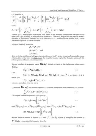
( , ) ( ) ( , ) ( ) ( ) ( , ) ( ) ( , ) ( ) 0 0 0 0
1
0
1
0
1 f z P z z A z f z P z z g z P z z g z
dz
d
P z z
That
is,
[ ( , ) ( )] ( , ) ( ) 0 0 0
1 P z z f z P z z g z
dz
d
or
[ ( , ) ( )] ( , ) ( ) 0 0 0 P z z f z P z z g z
dz
d
( , ) ( ) ( , ) ( ) ( ) 0 0 0
0
P z z f z P z g d f z
z
z
4.17
For the boundary value problem,
P z z f z P z z P z g d
f z P z z f z P z z P z g d
z
z
z
z
( , ) ( ) ( , ) ( , ) ( )
( ) ( , ) ( ) ( , ) ( , ) ( )
0 0
1
0 0
0 0
1
0 0
0
0
4.18
But, ( , ) ( , ) ( , ) ( , ) ( , ) 0 0 0
1 P z z P z P z z P z P z
Exchanging z and 0 z ,
( , ) ( , ) ( , ) ( , ) ( , ) 0 0 0 0
1 P z z P z P z z P z P z
Thus,
z
z
f z P z z f z P z g d
0
( ) ( , ) ( ) ( , ) ( ) 0 0 0 4.19
But from the definition,
z
P(z, ) exp( A(y)dy
So, equation (5.19) becomes
z
z
A y dy
f z P z z f z g e z d
0
( )
0 0 0 ( ) ( , ) ( ) ( )
4.20
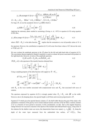
Next, we subdivide the shallow layer below the earth’s surface into twenty parallel slabs that are in welded
contact and each is of thickness 5m. Each subdivision is assumed to be homogeneous within which elastic
parameters , and density, are assumed to be constant. Regarding 0 z z as the earth’s surface, the
depth of the slabs below 0 z z is respectively 1 2 20 z z , z ,..., z . Thus, for
, 1,2,...,20 1 z z z s s s
( , ) exp[ ( )( ). s s 1 s 1 s P z z A z z z
So, for 1 s s z z z , equation (5.20) gives
10. Analytical And Numerical Modelling Of Layer...
www.ijmsi.org 27 | P a g e
1
( ) ( , ) ( ) ( )exp[ ( )( )] 1 0 0 1
s
s
z
z
s s s s f z P z z f z g z A z z z dz
4.21
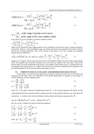
In numerical computation of the surface displacement components of the layer, we have used the Sylvester’s
interpolation formula (Bullen & Bolt, 1985) to obtain for each slab 1 s s z z z ,
21 22
11 12
1
exp[ ( )( )]
P P
P P
A z z zr r 4.22
where
s s s
s s s s s s s s s s s s
h z z
P Cosh h P h Sinh h P Sinh h P Cosh h
1
21 22
1
11 12 ( ); ( ) ( ); ( ) ( ); ( );
an
d s is the value of in 1 s s z z z . Similar results also hold for s .
V. WAVE INTERACTION WITH THE SHORELINE
In this consideration, we investigate the geophysical phenomenon which give rise to the intermediate
frequency range of the microseismic frequency. This frequency range is constantly observed in the series of
analysed gravity water waves and microseisms energy spectrum. In previous attempts, Darbyshire and Okeke
(1969) proposed a model of normal incident and reflected waves on a rocky coastline. Okeke (1972, 1985)
improved on this by assuming that the angle of incidence ranges from 0 to
2
. However, the reflected wave
energy was neglected in the computation. Okeke and Asor (2000) finally generalized the two successful
attempts. The last generalized theory is now used to study the phenomena of the observed micro-scale seismic
oscillations in the range of the intermediate frequency.
In this study, the technique initiated by Darbyshire and Okeke (1969) will be exploited and further generalized.
Let the subscripts i and r refer to the incident and reflected wave components along the coastline respectively.
Let i r k k k be the wave number difference. We now divide k in n sub-divisions each of width p k .
Thus, p k nk
For the incident modes, the spectral amplitudes for the sub-divisions are n h ,h ,..., h 1 2 and for the reflected
modes, they are n g , g ,..., g 1 2 .
In this study, ( , , ) i i i h h R and ( , , ) r r r g g R
The definitions incorporate the angle of incidence i and that of reflection r . Generally, they are usually
regarded as equal. The resultant spectral amplitude is obtained by the convolution of the two spectral
components. That is,
n
r
i r ir
n
i
h g
1 1
where
r i
r i
ir
ir
0 when
1 when
and ir is the Kronecker delta. Physically, r i corresponds to the case
of constructive interference, r i that of destructive interference.
This study concentrates only on the case of constructive interference, so, when, r i , r r f g h R where
f R is the reflection coefficient and is taken as the ensemble average for angles of incidence and reflection.
Thus,
g h = R g2
f i
n
i=1
i i
n
i=1
and
11. Analytical And Numerical Modelling Of Layer...
www.ijmsi.org 28 | P a g e
f p
2
f i
n
i=1
R g = R S ( ,K , ) nK 1 0 , m K K 0 . 5.1
0 K is the wave number of gravity water wave mode, m K is the low wave number component of the water
wave which is small enough to resonate the seismic modes of the seabed, m K K K 0 , i.e. K [,] .
( , , ) 1 0 S K is the spectral amplitude.
To a reasonable degree of accuracy, the power spectrum of a system is proportional to the square of the
amplitude spectrum. Thus for 0 K ,
p f p S (K ,, ) R S (K ,, )nK 0
2
0 1 5.2
S p( K0 , , ) is the power spectrum of the sea wave. The inequality immediately before equation (5.2)
implies that both high and low phase velocity wave number components arising from the linear modulation of
the gravity (water) wave bottom pressure are now activated (Hasselmann, 1963).
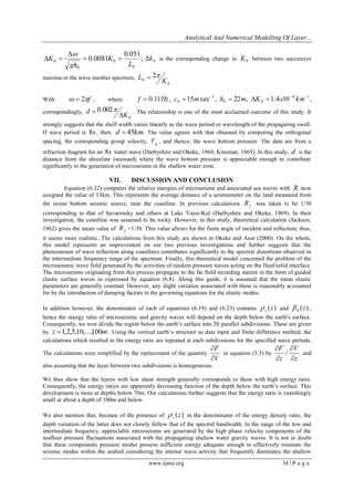
Our model sea wave is that which approaches a shoreline at an angle . Here, , is measured from the line
normal to the shoreline. The sea bottom is uniformly sloping but not necessarily parallel to the shoreline. The
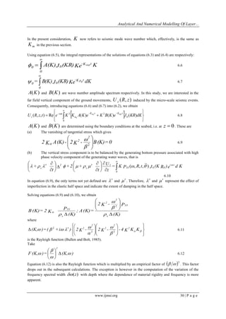
constant , is the gradient of slope. Then, following Okeke (1972, 1985), the wave bottom pressure in this
study takes the form
t.
g
R
J 2
R
d
P33 = w g 0
cos
2
cos
5.3
2
0 < <
, w = water density, R is the radial distance measured from the centre of the generating source,
d is the width of the shelf which includes the breaking zone as measured from the shoreline, 0 J is a zero
order Bessel function of the first kind, g is the acceleration due to gravity.
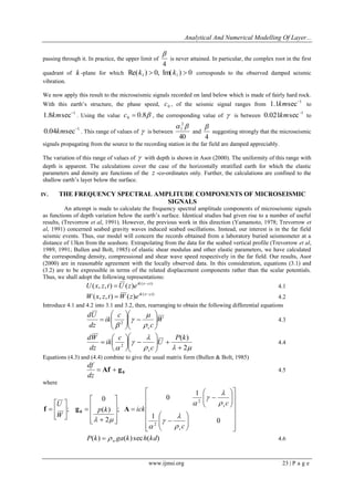
Typical Orthogonal (direction of wavenumbers, vectors perpendicular
to the wave crest)
Bottom Contour
Typical Wavecrest
Shoreline
Fig.1 Reflection of waves along the shoreline….
The components of the Fourier-Bessel coefficients corresponding to equation (5.3) are
12. Analytical And Numerical Modelling Of Layer...
www.ijmsi.org 29 | P a g e
2
cos
K + K
g
J
K + K
d
CH(K, , )=
0 m
2 -1
0
0 m 2
1
2
1
-
5.4
2
cos
K - K
g
J
K - K
d
SH(K, , )=
0 m
2 -1
0
0 m 2
1
2
1
-
5.5
, in the range of low wave number modes
, in the range of gravity wa ter waves. 0
m K
K
K
In the range of very low frequency or primary frequency modes,
1
K - K
g
J
K +K
g
J
0 m
2 -1
0
0 m
2 -1
0
5.6
Okeke (1972) utilized the above approximations in the calculations involving the range of primary frequency
microseisms. However, in the intermediate range, the whole expressions in the equations (5.4) and (5.5) will be
used in the on-going calculations. Thus, with variation of one percent in the wave number, the amplitude
spectral density is defined by
2
K
g
J
K
2 d
=
2
S K , , = CH ( K , ) + SH ( K , ) co s 2
0
-1
2
0
0
2 -1
2
0
2
0
2
0
2
1
Cos
5.7
Equation (5.7) suggests that the spectral density favours the moderate breaker zone and a rather gently sloping
beach. The equation gives the power of pressure wave per unit wave number in the water layer, which in the
present study is inversely proportional to the gravity wave number of the exciting source, i.e. proportional to the
wavelength of the exciting source (i.e. shallow water swell). This conclusion is quantitatively in agreement with
the observed behaviour of microseisms and the generating sea waves.
VI. STRESS WAVES IN AN ELASTIC AND HOMOGENOUS HALF SPACE
In this section, we review the base equations governing the evolutions of stress waves in an elastic and
homogeneous half space. Here, the components of the ground displacement in response to the passage of
seismic oscillations are thus usually given by
R z
+
R
U =
2
R
6.1
R
R
1
-
R
-
z
U = 2
2
z
6.2
where R U is the radial component of displacement whilst Uz is the vertical component. and are still
scalar potential functions associated with the compressional wave with speed and shear wave with speed
respectively. z as before is the vertical coordinate with the related radial distance represented by R .
Take Re{ ( , ) } 0
i t R z e and Re{ ( , ) } 0
i t R z e
then, 0 and 0 respectively satisfy the following equations
+ = 0
z
+
R
R
1
+
R
2 0
0
2
2
2
2
2
6.3
+ = 0
z
+
R
R
1
+
R
2 0
0
2
2
2
2
2
6.4
where
2
0
2
2
2
0
2
2 2 K = K + = K + 0 0
6.5
13. Analytical And Numerical Modelling Of Layer...
www.ijmsi.org 30 | P a g e
In the present consideration, K now refers to seismic mode wave number which, effectively, is the same as
m K in the previous section.
Using equation (6.5), the integral representations of the solutions of equations (6.3) and (6.4) are respectively:
A(K)J (KR)Ke K -K z
0
0
0
0
6.6
= B(K) J (KR)Ke dK -K z
0
0
0
0
6.7
A(K) and B(K) are wave number amplitude spectrum respectively. In this study, we are interested in the
far field vertical component of the ground movements, U (R, z) z induced by the micro-scale seismic events.
Consequently, introducing equations (6.6) and (6.7) into (6.2), we obtain
0
0
2 2 ( , , ) Re ( ) 0 ( ) 0 ( )
0
U R z t e K K A K e K B K e J KR dK
i t K z K z
z
6.8
A(K) and B(K) are determined using the boundary conditions at the seabed, i.e. at z 0 . These are
(a) The vanishing of tangential stress which gives
2 K A (K) - 2K - B (K) = 0
2
2
2
6.9
(b) The vertical stress component is to be balanced by the generating bottom pressure associated with high
phase velocity component of the generating water waves, that is
= K P R t J (K R ) e d K
z
U
t
+ 2 +
t
+ i t
33 0 0
0
z
s
2
s
(, , , )
6.10
In equation (6.9), the only terms not yet defined are and . Therefore, and represent the effect of
imperfection in the elastic half space and indicate the extent of damping in the half space.
Solving equations (6.9) and (6.10), we obtain
(K)
2K - P
; A (K) =
(K)
P
B (K) = 2 K
s
33
2
2
s
33
2
where
(K, ) = ( + i ) 2 K - 2 K - - 4 K K K 2
2
2
2
2
2 2
2
6.11
is the Rayleigh function (Bullen and Bolt, 1985).
Take
F (K, ) = (K, )
2
6.12
Equation (6.12) is also the Rayleigh function which is multiplied by an empirical factor of 2 . This factor
drops out in the subsequent calculations. The exception is however in the computation of the variation of the
frequency spectral width (z) with depth where the dependence of material rigidity and frequency is more
apparent.
14. Analytical And Numerical Modelling Of Layer...
www.ijmsi.org 31 | P a g e
In the areas outside the shallow water zone, 0 33 P . Thus, if equations (6.9) and (6.10) are to be consistent,
F(K,) must vanish identically. Consequently, in verifying the wave number,
(K, ) + ( K ) = 0
K
F
F(K, ) = F(K , ) + K 2
K=K
6.13
From which
(K , )
K
F
- F (K , )
K
6.14
where K is the value of K for which equation (6.13) is satisfied.
In the evaluation of the numerator of equation (6.14), we work in terms of the group velocity, V , of the seismic
modes. Thus,
V
F
V
F
K
C
V
K
V
F
=
K
F
m
m
65.3 6.15
(Here, m C = 2.8 km sec-1). When K = 0.30km-1 (wave length of about 20.9km), gives
K = 3.1 10-4 km-1 6.16
Equation (6.16) gives a result which suggests that the spectrum (energy and amplitude) of the underlying elastic
solid is highly peaked.
However, wave energy or amplitude spectrum is usually calculated in terms of frequencies rather than wave
numbers. Thus, if is the frequency bandwidth shown in figure 2 below, from equation (6.13),
Figure 2. Sketch of Wave Energy as a function of frequency, , (in Hz)
F(K, ) 0 6.17
we obtain approximately that,
( , ) ( , ) ( ) 0 2
F
F K F K
and then, as 0
E()
15. Analytical And Numerical Modelling Of Layer...
www.ijmsi.org 32 | P a g e
4
1
2
1
6
1
4
1
2
1
2
2 2
2 4
2 4 6
2 2
256 64 6
4 96 128 16
256 64 6
96 128 16
( , )
( , )
m m
c c
c c c
k
F k
F K
6.18
(In Hz.)
2
1, 1
f
c
, m and m are the dominant wavelength and peak frequency
respectively.
Equation (6.18) is here used in studying the shallow layer below the earth's surface. So, we have neglected the
effect of which gives the rate of decay of seismic vibrations in the horizontal direction.
In a horizontally stratified shallow structure below the earth's surface, (z) and (z) s s .
Therefrom, (z) . Further, m is about 30km and is about 1.8km/sec in the upper earth's layer
made of soft rock. Thus, despite the factor
2 on the numerator of the right hand side of equation (6.18),
(z) 1. The inequality applies at all depths below the earth's surface over which microseismic signals are
detectable. However, the factor
2 suggests the strong dependence of (z) on the layer rigidity and the
peak wavelength m .
The foregoing statement is confirmed by the numerical calculations depicting the vertical profile of (z) .
The data source is the shear velocity (z) and density (z) s vertical structures extrapolated from the
reference shear wave velocity profile (Bullen and Bolt, 1985; Yamamoto and Torii, 1986; Trevorrow and
Yamamoto, 1991). Thus, figure 2, compares well with the records from the local data. The computed values of
f as function of z are shown in Asor (2000).
If z 1.1m and the period is 8seconds, then,
2 8 1 2 ( ) 16.9 10 ( sec ) x rad . These data are those
frequently used for theoretical calculations involving the peak energy of the solid vertical displacement in
response to the passage of the seismic events. Hence, z 1.1m suggests the likely depth of burial of a land-based
seismometer. Calculations from equation (6.8) further verify that (z) is a decreasing function of the
material rigidity for
2 2
1
1
m T
O
, where m T is the period of the peak,
m
m T
2 .
Consequently, the computed values of f as function of z depicts the form of the vertical structure of the
elastic medium to a depth of about 100m below the earth's surface in the locality (Trevorrow et. al., 1989).
Now,
s
2 2
,
s
for the damping coefficient, (Okeke, 1972).
Eventually, equation (6.8) takes the form
16. Analytical And Numerical Modelling Of Layer...
www.ijmsi.org 33 | P a g e
dK
F(K, )
K J (KR)P (K, , )
U (R, (-0.11 t)= 2
s
0 33
0
z
) exp 6.19
1 1
0
1
0 , 20 100 , 0.1 0.4 K K K km K km K km m m
For large R , we use the asymptotic form of J0 (KR) which is
4
cos KR
KR
2
J (KR) =
2
1
0
6.20
Applying the stationary phase method in seismology (Ewing et. al., 1957) to equation (6.19) using equation
(6.20), then,
(K - K )
F/ K
K
R
2
2 P ( K , )
U (R, ) (-0.11 t) = m
k
2
1
s
33 0
z
exp 6.21
where ( ) m K K is the delta function. k
implies that the summation is over all possible values of k in
the spectrum. However, the contribution to equation (6.21) will come from those values of K that are the roots
of F(K,) 0 .
We now evaluate the amplitude spectrum in the K -plane for the left and right hand sides of equation (6.21).
The convolution theorem applied to Hankel's transform is used to evaluate the power associated with product on
the right-hand side. However, in terms of the amplitude spectrum,
( , , ) ( , , ) ( , ) 0 u p p S K S K H K 6.22
( , ) p H K is the spectrum of the transfer function obtained from
(K - K )
K
F
K
R
2
p
k
2
1
Using a sampling property of the delta function with support at p K K ,
K
F
R
2K
H ( K , ) =
-2
K = K
p
2
p
6.23
K i K K K
K
F
2
1 1
4 [4
2 2
2 2 2
2
6.24
with K as the wave number associated with compressional wave and K that associated with wave of
rotation.
The spectrum expressed by equation (6.23) is strongly peaked when p m K K with K as the width.
However, due to the damping factor, the spectral height is still finite and inversely proportional to R .
Equation (5.7) which gives the spectral density contains d , the shelf width. Because the goal of this study is the
quantitative evaluation of the gravity waves (water) induced seismic activities in the far field, a realistic estimate
of d as a function of wave period is necessary. In this consideration, we take as the angular frequency
change between two successive maxima in the spectra of the incident and reflected beach waves. Using some of
the relations for the shallow water sea waves, the characteristic linear wave speed, 0 0 c gh , 0 h being the
depth of the water layer measured from the undisturbed free surface, 0
2
0
2 K c . Thus,
17. Analytical And Numerical Modelling Of Layer...
www.ijmsi.org 34 | P a g e
;
0.051
0.0081
0
0
0
0 L
K
gh
K
0 k is the corresponding change in 0 K between two successive
maxima in the wave number spectrum,
0
0
2
K
L
With 2f , where
4 1
0 0
1
0 0.11 , 15 sec , 22 , 1.4 10 f Hz c m h m K x km ,
correspondingly,
0
0.002
K
d
. The relationship is one of the most acclaimed outcome of this study. It
strongly suggests that the shelf width varies linearly as the wave period or wavelength of the propagating swell.
If wave period is 8s , then, d 45km. The value agrees with that obtained by computing the orthogonal
spacing, the corresponding group velocity, g V , and thence, the wave bottom pressure. The data are from a
refraction diagram for an 8s water wave (Darbyshire and Okeke, 1969; Kinsman, 1965). In this study, d is the
distance from the shoreline (seaward) where the wave bottom pressure is appreciable enough to contribute
significantly to the generation of microseisms in the shallow water zone.
VII. DISCUSSION AND CONCLUSION
Equation (6.22) computes the relative energies of microseisms and associated sea waves with R now
assigned the value of 13km. This represents the average distance of a seismometer on the land measured from
the ocean bottom seismic source, near the coastline. In previous calculations f R was taken to be 1/30
corresponding to that of Savarensky and others at Lake Yussi-Kul (Darbyshire and Okeke, 1969). In their
investigation, the coastline was assumed to be rocky. However, in this study, theoretical calculation (Jackson,
1962) gives the mean value of f R =1/38. This value allows for the finite angle of incident and reflection; thus,
it seems more realistic. The calculations from this study are shown in Okeke and Asor (2000). On the whole,
this model represents an improvement on our two previous investigations and further suggests that the
phenomenon of wave reflection along coastlines contributes significantly to the spectral distortions observed in
the intermediate frequency range of the spectrum. Finally, this theoretical model concerned the problem of the
microseismic wave field generated by the activities of random pressure waves acting on the fluid/solid interface.
The microseisms originating from this process propagate to the far field recording station in the form of guided
elastic surface waves as expressed by equation (6.8). Along this guide, it is assumed that the mean elastic
parameters are generally constant. However, any slight variation associated with these is reasonably accounted
for by the introduction of damping factors in the governing equations for the elastic modes.
In addition however, the denominator of each of equations (6.19) and (6.23) contains (z) s and ( ) 0 z ,
hence the energy ratio of microseismic and gravity waves will depend on the depth below the earth's surface.
Consequently, we now divide the region below the earth’s surface into 20 parallel subdivisions. These are given
by z 1,2,5,10,...1, 00m. Using the vertical earth’s structure as data input and finite difference method, the
calculations which resulted in the energy ratio are repeated at each subdivisions for the specified wave periods.
The calculations were simplified by the replacement of the quantity
V
F
in equation (5.3) by
z
V
/
z
F
and
also assuming that the layer between two subdivisions is homogeneous.
We thus show that the layers with low shear strength generally corresponds to those with high energy ratio.
Consequently, the energy ratios are apparently decreasing function of the depth below the earth’s surface. This
development is more at depths below 70m. Our calculations further suggests that the energy ratio is vanishingly
small at about a depth of 100m and below.
We also mention that, because of the presence of (z) s in the denominator of the energy density ratio, the
depth variation of the latter does not closely follow that of the spectral bandwidth. In the range of the low and
intermediate frequency, appreciable microseisms are generated by the high phase velocity components of the
seafloor pressure fluctuations associated with the propagating shallow water gravity waves. It is not in doubt
that these components pressure modes possess sufficient energy adequate enough to effectively resonate the
seismic modes within the seabed considering the intense wave activity that frequently dominates the shallow
18. Analytical And Numerical Modelling Of Layer...
www.ijmsi.org 35 | P a g e
water areas. Equation (6.22) governs this process with ( , , ) 0 S K p as the functional representative of the
water wave energy spectrum. On the other hand, ( , ) 0 H K p is the coupling function whose role is to
communicate the gravity wave energy to the seismic modes.
However, the double frequency microseisms are not related to the linear modulation of the seafloor
randomly distributed seawave bottom pressure fluctuations. Instead, the energy input in this case is derived from
non-linear interactions among the components of the seawaves. The amplitude and energy spectra of the
interacting seawaves in shallow water need to be derived. Successful attempts had been made by Darbyshire and
Okeke (1969). More promising is the model developed by Okeke (1978). This is a one-dimensional solution and
it only needs a generalization to two-dimensions to produce the desired result.As already stated, the computed
results arising from this study are nearer to the observed than previous attempts. However, these results could be
significantly improved if the energy of the second order wave effects is incorporated.
REFERENCES
[1] Asor V.E. and Okeke E.O. 1998: The comments on the spectrum of microseismic frequencies, J. of Nigeria Math Phys. 2, 56-61.
[2] Banerji, S.K. (1930); Microseisms associated with disturbed weather. Philosophical Transactions of the Royal Society of London
229: 287-328
[3] Bullen K.E. and Bolt B.A; 1985: An Introduction to the theory of Seismology Cambridge University Press.
[4] Darbyshire J; 1950: Identification of activity with sea waves, Proc. R. Soc. A202, 439-448.
[5] Darbyshire J and Okeke E.O.; 1969: A Study of Microseisms Recorded in Anglesey, Geophys. J. R. Astro. Soc. 17, 63-92.
[6] Gherzi, E. (1932); Cyclones and Microseisms. Gerl. Beitr. Gph. 36: 20-3
[7] Goodman, D., Yamamoto T, Trevorrow M, Abbott. C, Target. A, Badly, M. and Ando, K; 1989. Direction spectra observations of
seafloor microseisms from an ocean bottom seismometer array. J. Acoust. Soc. Am. 86(6) 2309 - 2317.
[8] Gutenberg, B. (1958B); Microseisms. Advances in Gph. 5, 53-92
[9] Hasselmann, K; 1963: A Statistical Analysis of the Generation of the Microseisms. Rev. Geophys; 1, 177-210.
[10] Haubrick, R.A. and MacKenzie, G.S. (1965); Earth Noise, 5 to 500 millicycles per second. Journal of Geophysical Research,
70:1429-40
[11] Hinde, B and Hartley, A; 1965: Comparative Spectra of Sea Waves and Microseisms, Nature, Lond. 205, 1100.
[12] Howell, B.F. Jr. (1990); An Introduction to Seismological Research, History and Development. Cambridge University Press (143p),
pp. 131ff.
[13] Kinsman B.; 1965: Wind waves, Prentice - Hall, Inc.
[14] Kurosh A; 1980: Higher Algebra MIR Publishers (Moscow).
[15] Longuet-Higgins M.S., 1950: A Theory of the Origin of Microseisms, Phil. Trans. R. Soc. A243, 1 - 35.
[16] Okeke E.O; 1972: A Theoretical Model of Primary Frequency Microseisms, Geophy. J.R. astr. Soc. 27, 289 - 299.
[17] Okeke E.O; 1978: The operation of the second order wave modes on a uniformly sloping beach, Geof. Intern. Vol. 17, No. 2 253 -
263.
[18] Okeke, E.O., Adejayan C. and Asor, V.E. (1999); On the evolutions of the ocean wave generated low frequency seismic noise. J.
Nig. Ass. Math. Phys., 3, pp. 290-298.
[19] Okeke E.O and Asor V.E. 1998: Further on the Damping of low Frequency Seismic Waves in a Semi-Infinite Elastic Medium, J. of
Nigeria Math Phys. 2, 48 - 55.
[20] Okeke E.O. and Asor V.E. 2000: On the microseisms associated with coastal sea waves, Geophys. J. Int.141, pp 672-678
[21] Ramirez, J.E. (1940); An experimental investigation of the nature and origin of microseisms. Bulletin of the Seismological Society
of America 30: 35-84, 139-78
[22] Sheriff, R. E. (1991); Encyclopedic dictionary of exploration geophysics.
[23] Trevorrow M.V, Yamamoto T., Badiey H., Turgut, A and Cormer C. 1988a: Experimental Verification of Seabed Shear Modulus
Profile Inversion, Geophy. Journal 93(3), 419 - 436.
[24] Trevorrow M.V. and Yamamoto T. 1991: Summary of Marine Sedimentary Shear Modulus and Acoustic Speed Profile Results
Using a Gravity Wave Inversion Technique. J. Acoust. Soc. Am. 90(1) 441 - 456.
[25] Trevorrow M.V, Yamamoto T., Turgut A., Goodman D and Badiey, H. 1989: Very Low Frequency Ocean Bottom Ambient
Seismic Noise, Marine Geophy. Research, 11, 129 - 152.
[26] Van Straten, F.W. (1953); Storm and surf microseisms. In symposium on Microseisms, ed. J. T. Wilson and F. Press, pp. 94-108.
Washinton: U.S. Natl. Acad. Sci.
[27] Wiechart, E. (1904); Verhandlungen der zweiten internationalen seismologischen Konferenz, Strassburg, 1903. Beitr. Gph. Erganz.
2: 41-3
[28] Yamamoto T. 1977: Wave Induced Instability in Seabeds. Proc. A.S.C.E. Spec. Conf.: Coastal Sediments 77, Charleston, Sc.
[29] Yamamoto T. 1978: On the Response of a Poro-elastic bed to water waves. J. Fluid Mech. 87 part 1. 193 - 206.