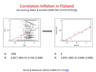
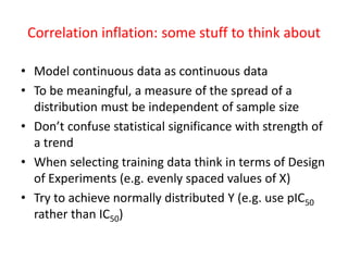
Accident and misadventure in property-based molecular design 
Peter W Kenny (blog) 
NEQUIMED-IQSC-USP 
Funding: FAPESPand CNPq
Hypothesis-driven molecular design and relationships between 
structures as framework for analysing activity and properties 
? 
Date of Analysis N DlogFu SE SD %increase 
2003 7 -0.64 0.09 0.23 0 
2008 12 -0.60 0.06 0.20 0 
Mining PPB database for carboxylate/tetrazole pairs suggested that bioisosteric replacement would 
lead to decrease in Fu . Tetrazoles were not synthesised even though their logP values are expected to 
be 0.3 to 0.4 units lower than for corresponding carboxylic acids. 
Hypothesis-driven versus prediction-driven molecular design: Kenny JCIM 2009 49:1234-1244 DOI 
Relationships between structures as framework for analyzing SAR/SPR: Kenny & Sadowski (2005) Methods and 
Principles in Medicinal Chemistry (Chemoinformatics in Drug Discovery, ed T Oprea) 2005, 23, 271-285 DOI 
Tetazole/carboxylate matched molecular pair analysis: Birch et al (2009) BMCL19:850-853 DOI
Some things that make drug discovery difficult 
•Having to exploit targets that are weakly-linked to human disease 
•Poor understanding and predictability oftoxicity 
•Inability to measure free (unbound) physiological concentrations of drug for remote targets (e.g. intracellular or on far side of blood brain barrier) 
Dansla merde, FBDD & Molecular Design blog :
TEP= [퐷푟푢푔푿,푡]푓푟푒푒 퐾푑 
Target engagement potential (TEP) 
A basis for pharmaceutical molecular design? 
Design objectives 
•Low Kdfor target(s) 
•High (hopefully undetectable) Kdfor antitargets 
•Ability to control[Drug(X,t)]free 
Kenny, Leitão& MontanariJCAMD 2014 28:699-710 DOI
Property-based design as search for ‘sweet spot’ 
Greenandredlinesrepresentprobabilityofachieving‘satisfactory’affinityand‘satisfactory’ADMETcharacteristicsrespectively.Thebluelineshowstheproductoftheseprobabilitiesandcharacterizesthe‘sweetspot’.Thiswayofthinkingaboutthe‘sweetspot’hassimilaritieswithmolecularcomplexitymodelproposedbyHannetal. 
Kenny & Montanari, JCAMD 2013 27:1-13 DOI
Euprefirominhacomida cozidae meus dados brutos….
Correlation 
•Strong correlation implies good predictivity 
–Beware of ‘experts’ who say, “I have observed a correlation so you must use my rule” (Actually, beware of experts and rules). 
•Multivariate data analysis (e.g. PCA) usually involves transformation to orthogonal basis 
•Applying cutoffs (e.g. MW restriction) to data can distort correlations 
•Noise in measurement and dynamic range impose limits on strength of correlation
Quantifying strengths of relationships between continuousvariables 
•Correlation measures 
–Pearson product-moment correlation coefficient (R) 
–Spearman's rank correlation coefficient () 
–Kendall rank correlation coefficient(τ) 
•Quality of fit measures 
–Coefficient of determination (R2) is the fraction of the variance in Y that is explained by model 
–Root mean square error (RMSE)
Drug-likeness ‘experts’ are usually shy about sharing their data but there is a way forward…
Preparation of synthetic data sets 
Add Gaussian noise (SD=10) to Y 
Kenny & Montanari(2013) JCAMD 27:1-13 DOI
Correlation inflation by hiding variation 
See Hopkins, Mason & Overington(2006) CurrOpinStructBiol16:127-136 DOI 
Leeson & Springthorpe(2007) NRDD 6:881-890 DOI 
Data is naturally binned (X is an integer) and mean value of Y is calculated for each value of X. In some studies, averaged data is only presented graphically and it is left to the reader to judge the strength of the correlation. 
R = 0.34 
R = 0.30 
R = 0.31 
R = 0.67 
R = 0.93 
R = 0.996
r 
N 
1202 
R 
0.247 ( 95% CI: 0.193| 0.299) 
N 
8 
R 
0.972 ( 95% CI: 0.846| 0.995) 
Correlation Inflation in Flatland 
See Lovering, Bikker& Humblet(2009) JMC 52:6752-6756 DOI 
Kenny & Montanari(2013) JCAMD 27:1-13 DOI
Masking variation with standard error 
“In each plot provided, the width of the errors bars and the difference in the mean values of the different categories are indicative of the strength of the relationship between the parameters.” Gleeson (2008) JMC 51:817-834 DOI 
Partition by value of X into four bins with equal numbers of data points and display 95% confidence interval for mean (green) and mean ±SD (blue) for each bin. 
R = 0.12 
R = 0.29 
R = 0.28 
Kenny & Montanari(2013) JCAMD 27:1-13 DOI
N 
Bins 
Degrees of Freedom 
F 
P 
40 
4 
3 
0.2596 
0.8540 
400 
4 
3 
12.855 
< 0.0001 
4000 
4 
3 
115.35 
< 0.0001 
4000 
2 
1 
270.91 
< 0.0001 
4000 
8 
7 
50.075 
< 0.0001 
ANOVA tests whether differences in mean values for different categories are significant 
ANOVA for binned synthetic data sets 
Kenny & Montanari(2013) JCAMD 27:1-13 DOI 
This analysis does not take account of ordering of categories (e.g. high, medium and low)
Know your data 
•Assays are typically run in replicate making it possible to estimate assay variance 
•Every assay has a finite dynamic range and it may not always be obvious what this is for a particular assay 
•Dynamic range may have been sacrificed for thoughputbut this, by itself, does not make the assay bad 
•We are likely to need to be able analysein-range and out-of-range data within single unified framework 
–See Lind (2010) QSAR analysis involving assay results which are only known to be greater than, or less than some cut-off limit. MolInf29:845-852 DOI
Correlation inflation: some stuff to think about 
•Model continuous data as continuous data 
•To be meaningful, a measure of the spread of a distribution must be independent of sample size 
•Don’t confuse statistical significance with strength of a trend 
•When selecting training data think in terms of Design of Experiments (e.g. evenly spaced values of X) 
•Try to achieve normally distributed Y (e.g. use pIC50rather than IC50)
Ligand efficiency metrics (LEMs) considered harmful
Introduction to ligand efficiency metrics (LEMs) 
•We use LEMs to normalize activity with respect to risk factors such as molecular size and lipophilicity 
•What do we mean by normalization? 
•We make assumptions about underlying relationship between activity and risk factor(s) when we define an LEM 
•LEM as measure of extent to which activity beats a trend? 
Kenny, Leitão& Montanari(2014) JCAMD 28:699-701 DOI 
Ligand efficiency metrics considered harmful, FBDD & Molecular design blog
Scaleactivity/affinity by risk factor 
LE = ΔG/HA 
Offsetactivity/affinity by risk factor 
LipE= pIC50ClogP 
Ligand efficiency metrics 
There is no reason that normalization of activity with respect to risk factor should be restricted to either of these functional forms. 
Kenny, Leitão& Montanari(2014) JCAMD 28:699-701 DOI
Use trend actually observed in data for normalization rather than some arbitrarily assumed trend 
Kenny, Leitão& Montanari(2014) JCAMD 28:699-701 DOI 
Can we accurately claim to have normalized a data set if we have made no attempt to analyseit?
There’s a reason why we say standardfree energy of binding 
DG= DHTDS= RTln(Kd/C0) 
•Adoption of 1 M as standard concentration is arbitrary 
•A view of a chemical system that changes with the choice of standard concentration is thermodynamically invalid (and, with apologies to Pauli, is ‘not even wrong’) 
Kenny, Leitão& Montanari(2014) JCAMD 28:699-701 DOI 
Efficient voodoo thermodynamics, FBDD & Molecular design blog
NHA 
Kd/M 
C/M 
(1/NHA)log10(Kd/C) 
10 
10-3 
1 
0.30 
20 
10-6 
1 
0.30 
30 
10-9 
1 
0.30 
10 
10-3 
0.1 
0.20 
20 
10-6 
0.1 
0.25 
30 
10-9 
0.1 
0.27 
10 
10-3 
10 
0.40 
20 
10-6 
10 
0.35 
30 
10-9 
10 
0.33 
Effect on LE of changing standard concentration 
Analysis from Kenny, Leitão& Montanari(2014) JCAMD 28:699-701 DOI 
Note that our article overlooked a similar analysis from 5 years earlier by 
Zhou & Gilson (2009) ChemRev 109:4092-4107 DOI
Scaling transformation of parallel lines by dividing Y by X 
(This is how ligand efficiency is calculated) 
Size dependency of LE in this example is consequence of non-zero intercept 
Kenny, Leitão& Montanari(2014) JCAMD 28:699-701 DOI
Affinity plotted against molecular weight for minimal binding elements against various targets in inhibitor deconstruction study showing variation in intercept term 
Data from Hajduk(2006) 
JMC 49:6972–6976 DOI 
Each line corresponds to a different target and no attempt has been made to indicate targets for individual data points. Is it valid to combine results from different assays in LE analysis? 
Kenny, Leitão& Montanari(2014) JCAMD 28:699-701 DOI
Offsetting transformation of lines with different slope and common intercept by subtracting X from Y 
(This is how lipophilic efficiency is calculated) 
Thankfully (hopefully?)lipophilicity-dependent lipophilic efficiency has not yet been ‘discovered’ 
Kenny, Leitão& Montanari(2014) JCAMD 28:699-701 DOI
Linear fit of ΔGto HA for published PKB ligands 
Data from Verdonk& Rees (2008) ChemMedChem3:1179-1180 DOI 
HA 
ΔG/kcalmol-1 
ΔG/kcalmol-10.87 (0.44 HA) 
R20.98 RMSE 0.43 
-ΔGrigid
Ligand efficiency, group efficiency and residuals plotted for PKB binding data 
Resid| GE 
GE 
Resid 
LE 
Residualsandgroupefficiencyvaluesshowsimilartrendswithpyrazole(HA=5) appearingasoutlier(GEiscalculatedusingΔGrigid).UsingresidualstocompareactivityeliminatesneedtouseΔGrigidestimate(seeMurray&Verdonk2002JCAMD16:741-753DOI)whichissubjecttouncertainty.
Use residuals to quantify extent to which activity beats trend 
•Normalize activity using trend(s) actually observed in data (this means we have to model the data) 
•All risk factors are treated within the same data-analytic framework 
•Residuals are invariant with respect to choice in standard concentration 
•Uncertainty in residuals is not explicitly dependent of value of risk factor (not the case for scaled LEMs) 
•Residuals can be used with other functional forms (e.g. non-linear and multi-linear) 
Kenny, Leitão& Montanari(2014) JCAMD 28:699-701 DOI
LEMs: some stuff to think about 
•Ligand efficiency as response of activity to risk factor 
•Need to model activity data if you want to normalize it 
•Using LEMs distorts data analysis unnecessarily

BrazMedChem2014

  • 1.
    Accident and misadventurein property-based molecular design Peter W Kenny (blog) NEQUIMED-IQSC-USP Funding: FAPESPand CNPq
  • 2.
    Hypothesis-driven molecular designand relationships between structures as framework for analysing activity and properties ? Date of Analysis N DlogFu SE SD %increase 2003 7 -0.64 0.09 0.23 0 2008 12 -0.60 0.06 0.20 0 Mining PPB database for carboxylate/tetrazole pairs suggested that bioisosteric replacement would lead to decrease in Fu . Tetrazoles were not synthesised even though their logP values are expected to be 0.3 to 0.4 units lower than for corresponding carboxylic acids. Hypothesis-driven versus prediction-driven molecular design: Kenny JCIM 2009 49:1234-1244 DOI Relationships between structures as framework for analyzing SAR/SPR: Kenny & Sadowski (2005) Methods and Principles in Medicinal Chemistry (Chemoinformatics in Drug Discovery, ed T Oprea) 2005, 23, 271-285 DOI Tetazole/carboxylate matched molecular pair analysis: Birch et al (2009) BMCL19:850-853 DOI
  • 3.
    Some things thatmake drug discovery difficult •Having to exploit targets that are weakly-linked to human disease •Poor understanding and predictability oftoxicity •Inability to measure free (unbound) physiological concentrations of drug for remote targets (e.g. intracellular or on far side of blood brain barrier) Dansla merde, FBDD & Molecular Design blog :
  • 4.
    TEP= [퐷푟푢푔푿,푡]푓푟푒푒 퐾푑 Target engagement potential (TEP) A basis for pharmaceutical molecular design? Design objectives •Low Kdfor target(s) •High (hopefully undetectable) Kdfor antitargets •Ability to control[Drug(X,t)]free Kenny, Leitão& MontanariJCAMD 2014 28:699-710 DOI
  • 5.
    Property-based design assearch for ‘sweet spot’ Greenandredlinesrepresentprobabilityofachieving‘satisfactory’affinityand‘satisfactory’ADMETcharacteristicsrespectively.Thebluelineshowstheproductoftheseprobabilitiesandcharacterizesthe‘sweetspot’.Thiswayofthinkingaboutthe‘sweetspot’hassimilaritieswithmolecularcomplexitymodelproposedbyHannetal. Kenny & Montanari, JCAMD 2013 27:1-13 DOI
  • 6.
  • 7.
    Correlation •Strong correlationimplies good predictivity –Beware of ‘experts’ who say, “I have observed a correlation so you must use my rule” (Actually, beware of experts and rules). •Multivariate data analysis (e.g. PCA) usually involves transformation to orthogonal basis •Applying cutoffs (e.g. MW restriction) to data can distort correlations •Noise in measurement and dynamic range impose limits on strength of correlation
  • 8.
    Quantifying strengths ofrelationships between continuousvariables •Correlation measures –Pearson product-moment correlation coefficient (R) –Spearman's rank correlation coefficient () –Kendall rank correlation coefficient(τ) •Quality of fit measures –Coefficient of determination (R2) is the fraction of the variance in Y that is explained by model –Root mean square error (RMSE)
  • 9.
    Drug-likeness ‘experts’ areusually shy about sharing their data but there is a way forward…
  • 10.
    Preparation of syntheticdata sets Add Gaussian noise (SD=10) to Y Kenny & Montanari(2013) JCAMD 27:1-13 DOI
  • 11.
    Correlation inflation byhiding variation See Hopkins, Mason & Overington(2006) CurrOpinStructBiol16:127-136 DOI Leeson & Springthorpe(2007) NRDD 6:881-890 DOI Data is naturally binned (X is an integer) and mean value of Y is calculated for each value of X. In some studies, averaged data is only presented graphically and it is left to the reader to judge the strength of the correlation. R = 0.34 R = 0.30 R = 0.31 R = 0.67 R = 0.93 R = 0.996
  • 12.
    r N 1202 R 0.247 ( 95% CI: 0.193| 0.299) N 8 R 0.972 ( 95% CI: 0.846| 0.995) Correlation Inflation in Flatland See Lovering, Bikker& Humblet(2009) JMC 52:6752-6756 DOI Kenny & Montanari(2013) JCAMD 27:1-13 DOI
  • 13.
    Masking variation withstandard error “In each plot provided, the width of the errors bars and the difference in the mean values of the different categories are indicative of the strength of the relationship between the parameters.” Gleeson (2008) JMC 51:817-834 DOI Partition by value of X into four bins with equal numbers of data points and display 95% confidence interval for mean (green) and mean ±SD (blue) for each bin. R = 0.12 R = 0.29 R = 0.28 Kenny & Montanari(2013) JCAMD 27:1-13 DOI
  • 14.
    N Bins Degreesof Freedom F P 40 4 3 0.2596 0.8540 400 4 3 12.855 < 0.0001 4000 4 3 115.35 < 0.0001 4000 2 1 270.91 < 0.0001 4000 8 7 50.075 < 0.0001 ANOVA tests whether differences in mean values for different categories are significant ANOVA for binned synthetic data sets Kenny & Montanari(2013) JCAMD 27:1-13 DOI This analysis does not take account of ordering of categories (e.g. high, medium and low)
  • 15.
    Know your data •Assays are typically run in replicate making it possible to estimate assay variance •Every assay has a finite dynamic range and it may not always be obvious what this is for a particular assay •Dynamic range may have been sacrificed for thoughputbut this, by itself, does not make the assay bad •We are likely to need to be able analysein-range and out-of-range data within single unified framework –See Lind (2010) QSAR analysis involving assay results which are only known to be greater than, or less than some cut-off limit. MolInf29:845-852 DOI
  • 16.
    Correlation inflation: somestuff to think about •Model continuous data as continuous data •To be meaningful, a measure of the spread of a distribution must be independent of sample size •Don’t confuse statistical significance with strength of a trend •When selecting training data think in terms of Design of Experiments (e.g. evenly spaced values of X) •Try to achieve normally distributed Y (e.g. use pIC50rather than IC50)
  • 17.
    Ligand efficiency metrics(LEMs) considered harmful
  • 18.
    Introduction to ligandefficiency metrics (LEMs) •We use LEMs to normalize activity with respect to risk factors such as molecular size and lipophilicity •What do we mean by normalization? •We make assumptions about underlying relationship between activity and risk factor(s) when we define an LEM •LEM as measure of extent to which activity beats a trend? Kenny, Leitão& Montanari(2014) JCAMD 28:699-701 DOI Ligand efficiency metrics considered harmful, FBDD & Molecular design blog
  • 19.
    Scaleactivity/affinity by riskfactor LE = ΔG/HA Offsetactivity/affinity by risk factor LipE= pIC50ClogP Ligand efficiency metrics There is no reason that normalization of activity with respect to risk factor should be restricted to either of these functional forms. Kenny, Leitão& Montanari(2014) JCAMD 28:699-701 DOI
  • 20.
    Use trend actuallyobserved in data for normalization rather than some arbitrarily assumed trend Kenny, Leitão& Montanari(2014) JCAMD 28:699-701 DOI Can we accurately claim to have normalized a data set if we have made no attempt to analyseit?
  • 21.
    There’s a reasonwhy we say standardfree energy of binding DG= DHTDS= RTln(Kd/C0) •Adoption of 1 M as standard concentration is arbitrary •A view of a chemical system that changes with the choice of standard concentration is thermodynamically invalid (and, with apologies to Pauli, is ‘not even wrong’) Kenny, Leitão& Montanari(2014) JCAMD 28:699-701 DOI Efficient voodoo thermodynamics, FBDD & Molecular design blog
  • 22.
    NHA Kd/M C/M (1/NHA)log10(Kd/C) 10 10-3 1 0.30 20 10-6 1 0.30 30 10-9 1 0.30 10 10-3 0.1 0.20 20 10-6 0.1 0.25 30 10-9 0.1 0.27 10 10-3 10 0.40 20 10-6 10 0.35 30 10-9 10 0.33 Effect on LE of changing standard concentration Analysis from Kenny, Leitão& Montanari(2014) JCAMD 28:699-701 DOI Note that our article overlooked a similar analysis from 5 years earlier by Zhou & Gilson (2009) ChemRev 109:4092-4107 DOI
  • 23.
    Scaling transformation ofparallel lines by dividing Y by X (This is how ligand efficiency is calculated) Size dependency of LE in this example is consequence of non-zero intercept Kenny, Leitão& Montanari(2014) JCAMD 28:699-701 DOI
  • 24.
    Affinity plotted againstmolecular weight for minimal binding elements against various targets in inhibitor deconstruction study showing variation in intercept term Data from Hajduk(2006) JMC 49:6972–6976 DOI Each line corresponds to a different target and no attempt has been made to indicate targets for individual data points. Is it valid to combine results from different assays in LE analysis? Kenny, Leitão& Montanari(2014) JCAMD 28:699-701 DOI
  • 25.
    Offsetting transformation oflines with different slope and common intercept by subtracting X from Y (This is how lipophilic efficiency is calculated) Thankfully (hopefully?)lipophilicity-dependent lipophilic efficiency has not yet been ‘discovered’ Kenny, Leitão& Montanari(2014) JCAMD 28:699-701 DOI
  • 26.
    Linear fit ofΔGto HA for published PKB ligands Data from Verdonk& Rees (2008) ChemMedChem3:1179-1180 DOI HA ΔG/kcalmol-1 ΔG/kcalmol-10.87 (0.44 HA) R20.98 RMSE 0.43 -ΔGrigid
  • 27.
    Ligand efficiency, groupefficiency and residuals plotted for PKB binding data Resid| GE GE Resid LE Residualsandgroupefficiencyvaluesshowsimilartrendswithpyrazole(HA=5) appearingasoutlier(GEiscalculatedusingΔGrigid).UsingresidualstocompareactivityeliminatesneedtouseΔGrigidestimate(seeMurray&Verdonk2002JCAMD16:741-753DOI)whichissubjecttouncertainty.
  • 28.
    Use residuals toquantify extent to which activity beats trend •Normalize activity using trend(s) actually observed in data (this means we have to model the data) •All risk factors are treated within the same data-analytic framework •Residuals are invariant with respect to choice in standard concentration •Uncertainty in residuals is not explicitly dependent of value of risk factor (not the case for scaled LEMs) •Residuals can be used with other functional forms (e.g. non-linear and multi-linear) Kenny, Leitão& Montanari(2014) JCAMD 28:699-701 DOI
  • 29.
    LEMs: some stuffto think about •Ligand efficiency as response of activity to risk factor •Need to model activity data if you want to normalize it •Using LEMs distorts data analysis unnecessarily