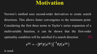
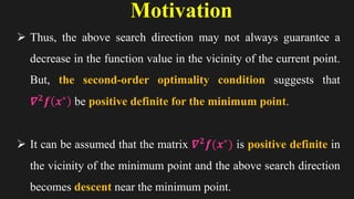
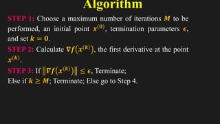
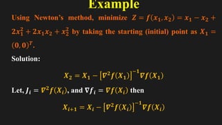
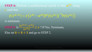
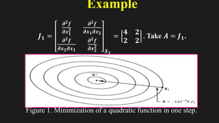
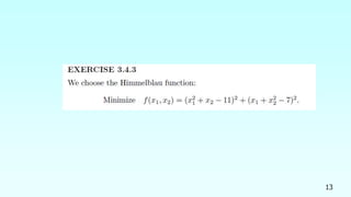
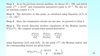
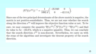
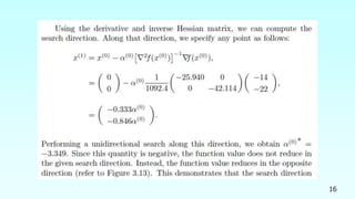
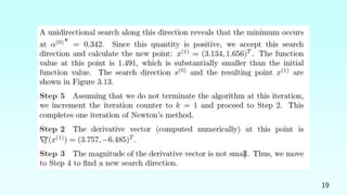
Newton’s Method for Multivariable
Optimization
Course Name: Optimization Techniques
Department of Mathematics
Amrita School of Engineering
Amrita Vishwa Vidyapeetham, Coimbatore
Outline
 Motivation
 Algorithm
 Example
 Remarks
Motivation
3
Newton’s method uses second-order derivatives to create search
directions. This allows faster convergence to the minimum point.
Considering the first three terms in Taylor’s series expansion of a
multivariable function, it can be shown that the first-order
optimality condition will be satisfied if a search direction
𝒔 𝒌
= − 𝜵𝟐
𝒇 𝒙 𝒌 −𝟏
𝜵𝒇 𝒙 𝒌
is used.
(𝟏)
Motivation
4
 If 𝜵𝟐𝒇 𝒙 𝒌 −𝟏
is positive semidefinite, the direction 𝒔 𝒌
must be descent.
 If 𝜵𝟐𝒇 𝒙 𝒌 −𝟏
is not positive definite, the direction 𝒔 𝒌 may
or may not be descent, depending on whether the quantity
𝛁𝒇 𝒙 𝒌 𝑻
𝜵𝟐
𝒇 𝒙 𝒌 −𝟏
𝜵𝒇 𝒙 𝒌
is positive or not.
Motivation
5
 Thus, the above search direction may not always guarantee a
decrease in the function value in the vicinity of the current point.
But, the second-order optimality condition suggests that
𝜵𝟐
𝒇 𝒙∗
be positive definite for the minimum point.
 It can be assumed that the matrix 𝜵𝟐𝒇(𝒙∗) is positive definite in
the vicinity of the minimum point and the above search direction
becomes descent near the minimum point.
Algorithm
6
STEP 1: Choose a maximum number of iterations 𝑴 to be
performed, an initial point 𝒙 𝟎 , termination parameters 𝝐,
and set 𝒌 = 𝟎.
STEP 2: Calculate 𝛁𝒇 𝒙 𝒌
, the first derivative at the point
𝒙 𝒌 .
STEP 3: If 𝜵𝒇 𝒙 𝒌
≤ 𝝐, Terminate;
Else if 𝒌 ≥ 𝑴; Terminate; Else go to Step 4.
Example
7
Using Newton’s method, minimize 𝒁 = 𝒇 𝒙𝟏, 𝒙𝟐 = 𝒙𝟏 − 𝒙𝟐 +
𝟐𝒙𝟏
𝟐
+ 𝟐𝒙𝟏𝒙𝟐 + 𝒙𝟐
𝟐
by taking the starting (initial) point as 𝑿𝟏 =
𝟎, 𝟎 𝑻.
Solution:
𝑿𝟐 = 𝑿𝟏 − 𝜵𝟐
𝒇 𝑿𝟏
−𝟏
𝜵𝒇 𝑿𝟏
Let, 𝑱𝒊 = 𝜵𝟐𝒇 𝑿𝒊 , and 𝛁𝒇𝒊 = 𝜵𝒇 𝑿𝒊 then
𝑿𝒊+𝟏 = 𝑿𝒊 − 𝜵𝟐𝒇 𝑿𝒊
−𝟏
𝜵𝒇 𝑿𝒊
https://www.youtube.com/SukantaNaya
kedu 8
STEP 4: Perform a unidirectional search to find 𝜶 𝒌 using
𝝐 such that
𝒇 𝒙 𝒌+𝟏
= 𝒇 𝒙 𝒌
− 𝜶 𝒌
𝜵𝟐
𝒇 𝒙 𝒌 −𝟏
𝜵𝒇 𝒙 𝒌
is minimum.
STEP 5: Is
𝒙 𝒌+𝟏 −𝒙 𝒌
𝒙 𝒌 ≤ 𝝐 ? If Yes, Terminate;
Else set 𝒌 = 𝒌 + 𝟏 and go to STEP 2.
Example
9
𝑱𝟏 =
𝝏𝟐𝒇
𝝏𝒙𝟏
𝟐
𝝏𝟐𝒇
𝝏𝒙𝟏𝝏𝒙𝟐
𝝏𝟐𝒇
𝝏𝒙𝟐𝝏𝒙𝟏
𝝏𝟐𝒇
𝝏𝒙𝟐
𝟐
𝑿𝟏
=
𝟒 𝟐
𝟐 𝟐
. Take 𝑨 = 𝑱𝟏.
Figure 1. Minimization of a quadratic function in one step.
10
Example
11
𝑱𝟏
−𝟏 =
𝟏
𝟐
−
𝟏
𝟐
−
𝟏
𝟐
𝟏
. 𝛁𝒇𝟏 =
𝟏 + 𝟒𝒙𝟏 + 𝟐𝒙𝟐
−𝟏 + 𝟐𝒙𝟏 + 𝟐𝒙𝟐 𝑿𝟏
=
𝟏
−𝟏
Hence, 𝑿𝟐 = 𝑿𝟏 − 𝑱𝟏
−𝟏𝛁𝒇𝟏 =
𝟎
𝟎
−
𝟏
𝟐
−
𝟏
𝟐
−
𝟏
𝟐
𝟏
𝟏
−𝟏
=
−𝟏
𝟏. 𝟓
𝛁𝒇𝟐 =
𝟏 + 𝟒𝒙𝟏 + 𝟐𝒙𝟐
−𝟏 + 𝟐𝒙𝟏 + 𝟐𝒙𝟐 𝑿𝟐
=
𝟎
𝟎
Remarks
12
 This method is suitable and efficient when the initial point is
close to the optimum point.
 Since, the function value is not guaranteed to reduce at every
iteration, the occasional restart of the algorithm from a different
point is often necessary.
13
14
15
16
17
18
19
20
21

Newton's Method for Multivariable.pdf.pptx

  • 1.
    Newton’s Method forMultivariable Optimization Course Name: Optimization Techniques Department of Mathematics Amrita School of Engineering Amrita Vishwa Vidyapeetham, Coimbatore
  • 2.
  • 3.
    Motivation 3 Newton’s method usessecond-order derivatives to create search directions. This allows faster convergence to the minimum point. Considering the first three terms in Taylor’s series expansion of a multivariable function, it can be shown that the first-order optimality condition will be satisfied if a search direction 𝒔 𝒌 = − 𝜵𝟐 𝒇 𝒙 𝒌 −𝟏 𝜵𝒇 𝒙 𝒌 is used. (𝟏)
  • 4.
    Motivation 4  If 𝜵𝟐𝒇𝒙 𝒌 −𝟏 is positive semidefinite, the direction 𝒔 𝒌 must be descent.  If 𝜵𝟐𝒇 𝒙 𝒌 −𝟏 is not positive definite, the direction 𝒔 𝒌 may or may not be descent, depending on whether the quantity 𝛁𝒇 𝒙 𝒌 𝑻 𝜵𝟐 𝒇 𝒙 𝒌 −𝟏 𝜵𝒇 𝒙 𝒌 is positive or not.
  • 5.
    Motivation 5  Thus, theabove search direction may not always guarantee a decrease in the function value in the vicinity of the current point. But, the second-order optimality condition suggests that 𝜵𝟐 𝒇 𝒙∗ be positive definite for the minimum point.  It can be assumed that the matrix 𝜵𝟐𝒇(𝒙∗) is positive definite in the vicinity of the minimum point and the above search direction becomes descent near the minimum point.
  • 6.
    Algorithm 6 STEP 1: Choosea maximum number of iterations 𝑴 to be performed, an initial point 𝒙 𝟎 , termination parameters 𝝐, and set 𝒌 = 𝟎. STEP 2: Calculate 𝛁𝒇 𝒙 𝒌 , the first derivative at the point 𝒙 𝒌 . STEP 3: If 𝜵𝒇 𝒙 𝒌 ≤ 𝝐, Terminate; Else if 𝒌 ≥ 𝑴; Terminate; Else go to Step 4.
  • 7.
    Example 7 Using Newton’s method,minimize 𝒁 = 𝒇 𝒙𝟏, 𝒙𝟐 = 𝒙𝟏 − 𝒙𝟐 + 𝟐𝒙𝟏 𝟐 + 𝟐𝒙𝟏𝒙𝟐 + 𝒙𝟐 𝟐 by taking the starting (initial) point as 𝑿𝟏 = 𝟎, 𝟎 𝑻. Solution: 𝑿𝟐 = 𝑿𝟏 − 𝜵𝟐 𝒇 𝑿𝟏 −𝟏 𝜵𝒇 𝑿𝟏 Let, 𝑱𝒊 = 𝜵𝟐𝒇 𝑿𝒊 , and 𝛁𝒇𝒊 = 𝜵𝒇 𝑿𝒊 then 𝑿𝒊+𝟏 = 𝑿𝒊 − 𝜵𝟐𝒇 𝑿𝒊 −𝟏 𝜵𝒇 𝑿𝒊
  • 8.
    https://www.youtube.com/SukantaNaya kedu 8 STEP 4:Perform a unidirectional search to find 𝜶 𝒌 using 𝝐 such that 𝒇 𝒙 𝒌+𝟏 = 𝒇 𝒙 𝒌 − 𝜶 𝒌 𝜵𝟐 𝒇 𝒙 𝒌 −𝟏 𝜵𝒇 𝒙 𝒌 is minimum. STEP 5: Is 𝒙 𝒌+𝟏 −𝒙 𝒌 𝒙 𝒌 ≤ 𝝐 ? If Yes, Terminate; Else set 𝒌 = 𝒌 + 𝟏 and go to STEP 2.
  • 9.
  • 10.
  • 11.
    Example 11 𝑱𝟏 −𝟏 = 𝟏 𝟐 − 𝟏 𝟐 − 𝟏 𝟐 𝟏 . 𝛁𝒇𝟏= 𝟏 + 𝟒𝒙𝟏 + 𝟐𝒙𝟐 −𝟏 + 𝟐𝒙𝟏 + 𝟐𝒙𝟐 𝑿𝟏 = 𝟏 −𝟏 Hence, 𝑿𝟐 = 𝑿𝟏 − 𝑱𝟏 −𝟏𝛁𝒇𝟏 = 𝟎 𝟎 − 𝟏 𝟐 − 𝟏 𝟐 − 𝟏 𝟐 𝟏 𝟏 −𝟏 = −𝟏 𝟏. 𝟓 𝛁𝒇𝟐 = 𝟏 + 𝟒𝒙𝟏 + 𝟐𝒙𝟐 −𝟏 + 𝟐𝒙𝟏 + 𝟐𝒙𝟐 𝑿𝟐 = 𝟎 𝟎
  • 12.
    Remarks 12  This methodis suitable and efficient when the initial point is close to the optimum point.  Since, the function value is not guaranteed to reduce at every iteration, the occasional restart of the algorithm from a different point is often necessary.
  • 13.
  • 14.
  • 15.
  • 16.
  • 17.
  • 18.
  • 19.
  • 20.
  • 21.