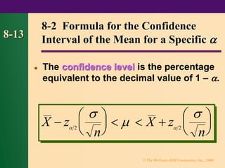
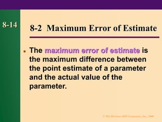
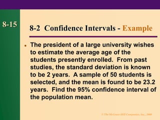
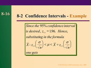
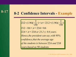
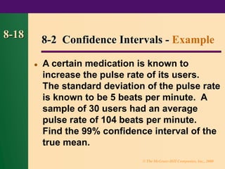
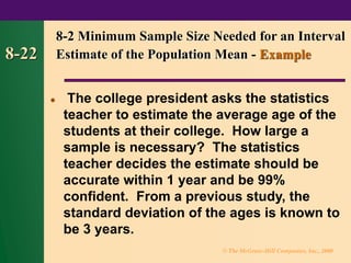
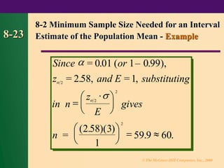
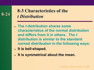
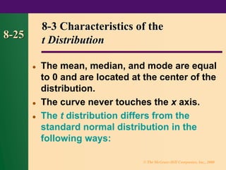
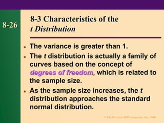
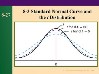
© The McGraw-Hill Companies, Inc., 2000
8-1
Chapter 8
Confidence Intervals
and Sample Size
© The McGraw-Hill Companies, Inc., 2000
8-2 Outline
⚫ 8-1 Introduction
⚫ 8-2 Confidence Intervals for the
Mean [ Known or n  30]
and Sample Size
⚫ 8-3 Confidence Intervals for the
Mean [ Unknown and n  30]
© The McGraw-Hill Companies, Inc., 2000
8-3 Outline
⚫ 8-4 Confidence Intervals and
Sample Size for Proportions
⚫ 8-5 Confidence Intervals for
Variances and Standard
Deviations
© The McGraw-Hill Companies, Inc., 2000
8-4 Objectives
⚫ Find the confidence interval for the
mean when  is known or n  30.
⚫ Determine the minimum sample
size for finding a confidence
interval for the mean.
© The McGraw-Hill Companies, Inc., 2000
8-5 Objectives
⚫ Find the confidence interval for the mean
when  is unknown and n  30.
⚫ Find the confidence interval for a proportion.
⚫ Determine the minimum sample size for
finding a confidence interval for a
proportion.
⚫ Find a confidence interval for a variance and
a standard deviation.
© The McGraw-Hill Companies, Inc., 2000
8-6
8-2 Confidence Intervals for the Mean
( Known or n  30) and Sample Size
X
A point estimate is a specific numerical
value estimate of a parameter. The best
estimate of the population mean is the
sample mean .

© The McGraw-Hill Companies, Inc., 2000
8-7
⚫ The estimator must be an unbiased
estimator. That is, the expected
value or the mean of the estimates
obtained from samples of a given
size is equal to the parameter being
estimated.
8-2 Three Properties of a Good
Estimator
© The McGraw-Hill Companies, Inc., 2000
8-8
⚫ The estimator must be consistent.
For a consistent estimator, as
sample size increases, the value of
the estimator approaches the value
of the parameter estimated.
8-2 Three Properties of a Good
Estimator
© The McGraw-Hill Companies, Inc., 2000
8-9
⚫ The estimator must be a relatively
efficient estimator. That is, of all
the statistics that can be used to
estimate a parameter, the relatively
efficient estimator has the smallest
variance.
8-2 Three Properties of a Good
Estimator
© The McGraw-Hill Companies, Inc., 2000
8-10 8-2 Confidence Intervals
⚫ An interval estimate of a parameter
is an interval or a range of values
used to estimate the parameter.
This estimate may or may not
contain the value of the parameter
being estimated.
© The McGraw-Hill Companies, Inc., 2000
8-11 8-2 Confidence Intervals
⚫ A confidence interval is a specific
interval estimate of a parameter
determined by using data obtained
from a sample and the specific
confidence level of the estimate.
© The McGraw-Hill Companies, Inc., 2000
8-12 8-2 Confidence Intervals
⚫ The confidence level of an interval
estimate of a parameter is the
probability that the interval
estimate will contain the
parameter.
© The McGraw-Hill Companies, Inc., 2000
8-13
⚫ The confidence level is the percentage
equivalent to the decimal value of 1 – .
8-2 Formula for the Confidence
Interval of the Mean for a Specific 
X z
n
X z
n
−





   +






 



2 2
© The McGraw-Hill Companies, Inc., 2000
8-14
⚫ The maximum error of estimate is
the maximum difference between
the point estimate of a parameter
and the actual value of the
parameter.
8-2 Maximum Error of Estimate
© The McGraw-Hill Companies, Inc., 2000
8-15
⚫ The president of a large university wishes
to estimate the average age of the
students presently enrolled. From past
studies, the standard deviation is known
to be 2 years. A sample of 50 students is
selected, and the mean is found to be 23.2
years. Find the 95% confidence interval of
the population mean.
8-2 Confidence Intervals - Example
© The McGraw-Hill Companies, Inc., 2000
8-16
Since the confidence
is desired z Hence
substituting in the formula
X z
n
X z
n
one gets
, ,
– +
2
95%
196
2 2
interval

 



=





   





. .
8-2 Confidence Intervals - Example
© The McGraw-Hill Companies, Inc., 2000
8-17
232
2
50
23.2
2
232 0 6 236 0 6
22 6 238
95%
22 6 238
50
. (1.96)( ) (1.96)( )
. . . .
. . or 23.2 0.6 years.
, ,
,
. .
, .
−   +
−   +
 



Hence the president can say with
confidence that the average age
of the students is between and
years based on students
8-2 Confidence Intervals - Example

50
© The McGraw-Hill Companies, Inc., 2000
8-18
⚫ A certain medication is known to
increase the pulse rate of its users.
The standard deviation of the pulse rate
is known to be 5 beats per minute. A
sample of 30 users had an average
pulse rate of 104 beats per minute.
Find the 99% confidence interval of the
true mean.
8-2 Confidence Intervals - Example
© The McGraw-Hill Companies, Inc., 2000
8-19
Since the confidence
is desired z Hence
substituting in the formula
X z
n
X z
n
one gets
, ,
– +
2
99%
258
2 2
interval

 



=





  






. .
8-2 Confidence Intervals - Example
© The McGraw-Hill Companies, Inc., 2000
8-20
104 (2.58)
5
30
104 (2.58)
5
30
104 2 4 104 2 4
1016 1064
99%
1016 106.4
−   +
−   +
 
. ( ) ( )
. .
. . .
, ,
,
.



Hence one can say with
confidence that the average pulse
rate is between and
beats per minute, based on 30 users.
8-2 Confidence Intervals - Example
© The McGraw-Hill Companies, Inc., 2000
8-21
8-2 Formula for the Minimum Sample Size
Needed for an Interval Estimate of the
Population Mean
.
,
.
n
z
E
where E is the error
of estimate
If necessary round the answer up
to obtain a whole number
=









2
2
maximum
© The McGraw-Hill Companies, Inc., 2000
8-22
⚫ The college president asks the statistics
teacher to estimate the average age of the
students at their college. How large a
sample is necessary? The statistics
teacher decides the estimate should be
accurate within 1 year and be 99%
confident. From a previous study, the
standard deviation of the ages is known to
be 3 years.
8-2 Minimum Sample Size Needed for an Interval
Estimate of the Population Mean - Example
© The McGraw-Hill Companies, Inc., 2000
8-23
Since or
z and E substituting
in n
z
E
gives
n
= . ( – . ),
= . , = ,
=
( . )( )




0 01 1 0 99
2 58 1
2 58 3
1
59 9 60
2
2
2
2
=












 = 
. .
8-2 Minimum Sample Size Needed for an Interval
Estimate of the Population Mean - Example
© The McGraw-Hill Companies, Inc., 2000
8-24
8-3 Characteristics of the
t Distribution
⚫ The t distribution shares some
characteristics of the normal distribution
and differs from it in others. The t
distribution is similar to the standard
normal distribution in the following ways:
⚫ It is bell-shaped.
⚫ It is symmetrical about the mean.
© The McGraw-Hill Companies, Inc., 2000
8-25
8-3 Characteristics of the
t Distribution
⚫ The mean, median, and mode are equal
to 0 and are located at the center of the
distribution.
⚫ The curve never touches the x axis.
⚫ The t distribution differs from the
standard normal distribution in the
following ways:
© The McGraw-Hill Companies, Inc., 2000
8-26
8-3 Characteristics of the
t Distribution
⚫ The variance is greater than 1.
⚫ The t distribution is actually a family of
curves based on the concept of
degrees of freedom, which is related to
the sample size.
⚫ As the sample size increases, the t
distribution approaches the standard
normal distribution.
© The McGraw-Hill Companies, Inc., 2000
8-27
8-3 Standard Normal Curve and
the t Distribution
© The McGraw-Hill Companies, Inc., 2000
8-28
⚫ Ten randomly selected automobiles
were stopped, and the tread depth of
the right front tire was measured. The
mean was 0.32 inch, and the standard
deviation was 0.08 inch. Find the 95%
confidence interval of the mean depth.
Assume that the variable is
approximately normally distributed.
8-3 Confidence Interval for the Mean
( Unknown and n < 30) - Example
© The McGraw-Hill Companies, Inc., 2000
8-29
⚫ Since  is unknown and s must replace
it, the t distribution must be used with
 = 0.05. Hence, with 9 degrees of
freedom, t/2 = 2.262 (see Table F in
text).
⚫ From the next slide, we can be 95%
confident that the population mean is
between 0.26 and 0.38.
8-3 Confidence Interval for the Mean
( Unknown and n < 30) - Example
© The McGraw-Hill Companies, Inc., 2000
8-30
8-3 Confidence Interval for the Mean
( Unknown and n < 30) - Example
Thus the confidence
of the population mean is found by
substituting in
X t
s
X t
s
n
0.32–(2.262)
0.08
10
(2.262)
0.08
10
95%
0 32
0 26 0 38
2 2
interval
−





   +











   +






 
 



.
. .
n
© The McGraw-Hill Companies, Inc., 2000
8-31
8-4 Confidence Intervals and
Sample Size for Proportions
Symbols Used in Notation
p population proportion
p read “p hat” sample proportion
p
X
n
and q
n X
n
or p
where X number of sample units that
possess the characteristic of
and n sample size
–
Proportion
interest
=
− =
= =
−
=
=
( )
  
.
1
© The McGraw-Hill Companies, Inc., 2000
8-32
⚫ In a recent survey of 150
households, 54 had central air
conditioning. Find and .
8-4 Confidence Intervals and Sample
Size for Proportions - Example
p̂ q̂
© The McGraw-Hill Companies, Inc., 2000
8-33
Since X and n then
p
X
n
and q
n X
n
or q p
=
54
150
= 0.36 = 36%
=
150 −54
150
= –
= =
=
=
−
= =
= − =
54 150
0 64 64%
1 1 0 36 0 64
,


.
  . . .
8-4 Confidence Intervals and Sample
Size for Proportions - Example
150
96
=
© The McGraw-Hill Companies, Inc., 2000
8-34

 

p
pq
n
p p
 
pq
n
−   +
8-4 Formula for a Specific Confidence
Interval for a Proportion
(z 2
) (z 2
)
© The McGraw-Hill Companies, Inc., 2000
8-35
⚫ A sample of 500 nursing applications
included 60 from men. Find the 90%
confidence interval of the true
proportion of men who applied to the
nursing program.
⚫ Here  = 1 – 0.90 = 0.10, and z/2 = 1.65.
⚫ = 60/500 = 0.12 and = 1– 0.12 = 0.88.
8-4 Specific Confidence Interval for
a Proportion - Example
p̂ q̂
© The McGraw-Hill Companies, Inc., 2000
8-36
8-4 Specific Confidence Interval for a
Proportion - Example
pq
n
 
Substituti ng in
p
pq
n
p p
we get
Lower limit
Upper limit
Thus
=
=
0.096 < p < 0.144 or 9.6% < p < 14.4%.

 

. ( . )
( . )( . )
.
. ( . )
( . )( . )
.
,
 
= −
= +
+ ( )
z 2
012 165
012 0 88
500
0 096
012 165
012 0 88
500
0144
− ( )
z 2
© The McGraw-Hill Companies, Inc., 2000
8-37
.
,
.
n pq
z
E
where E is the error
of estimate
If necessary round the answer up
to obtain a whole number
=






   2
2
maximum
8-4 Sample Size Needed for Interval
Estimate of a Population Proportion
© The McGraw-Hill Companies, Inc., 2000
8-38
⚫ A researcher wishes to estimate, with
95% confidence, the number of people
who own a home computer. A previous
study shows that 40% of those
interviewed had a computer at home.
The researcher wishes to be accurate
within 2% of the true proportion. Find
the minimum sample size necessary.
8-4 Sample Size Needed for Interval Estimate
of a Population Proportion - Example
© The McGraw-Hill Companies, Inc., 2000
8-39
Since z p
and q then n pq
z
E
= . , = . ,
= . ,
 

0 05 E
= . , = .
196 0 02 0 40
0 60
196
0 02
2304 96
Which, when rounded up is 2305 people
to interview.
2
2
2
2

  
.
.
.
=






= (0.40)(0.60)





 =
8-4 Sample Size Needed for Interval Estimate
of a Population Proportion - Example
© The McGraw-Hill Companies, Inc., 2000
8-40
8-5 Confidence Intervals for
Variances and Standard Deviations
⚫ To calculate these confidence intervals,
the chi-square distribution is used.
⚫ The chi-square distribution is similar to
the t distribution in that its distribution
is a family of curves based on the
number of degrees of freedom.
⚫ The symbol for chi-square is  2.
© The McGraw-Hill Companies, Inc., 2000
8-41
8-5 Confidence Interval for a
Variance
Formula for the confidence
for a
n s n s
d f n
right left
interval
variance
( ) ( )
. .
−
 
−
= −
1 1
1
2
2
2
2
2



© The McGraw-Hill Companies, Inc., 2000
8-42
Formula for the confidence
for a standard deviation
n s n s
d.f. n
right left
interval
( ) ( )
−
 
−
= −
1 1
1
2
2
2
2



8-5 Confidence Interval for a
Standard Deviation
© The McGraw-Hill Companies, Inc., 2000
8-43
⚫ Find the 95% confidence interval for the
variance and standard deviation of the
nicotine content of cigarettes
manufactured if a sample of 20 cigarettes
has a standard deviation of 1.6 milligrams.
⚫ Since  = 0.05, the critical values for the
0.025 and 0.975 levels for 19 degrees of
freedom are 32.852 and 8.907.
8-5 Confidence Interval for the
Variance - Example
© The McGraw-Hill Companies, Inc., 2000
8-44
The confidence
for the is found by
substituting in
n s n s
right left
95%
1 1
20 1
32852
20 1
8 907
15 55
2
2
2
2
2
2
2
2
2
interval
variance
( ) ( )
( )(1.6)
.
( )(1.6)
.
. .
−
 
−
−
 
−
 





8-5 Confidence Interval for the
Variance - Example
© The McGraw-Hill Companies, Inc., 2000
8-45
The confidence
for the standard deviation is
95% interval
15 55
12 2 3
. .
. .
 
 


8-5 Confidence Interval for the
Standard Deviation - Example

bman08.pdf statistics for health care workers

  • 1.
    © The McGraw-HillCompanies, Inc., 2000 8-1 Chapter 8 Confidence Intervals and Sample Size
  • 2.
    © The McGraw-HillCompanies, Inc., 2000 8-2 Outline ⚫ 8-1 Introduction ⚫ 8-2 Confidence Intervals for the Mean [ Known or n  30] and Sample Size ⚫ 8-3 Confidence Intervals for the Mean [ Unknown and n  30]
  • 3.
    © The McGraw-HillCompanies, Inc., 2000 8-3 Outline ⚫ 8-4 Confidence Intervals and Sample Size for Proportions ⚫ 8-5 Confidence Intervals for Variances and Standard Deviations
  • 4.
    © The McGraw-HillCompanies, Inc., 2000 8-4 Objectives ⚫ Find the confidence interval for the mean when  is known or n  30. ⚫ Determine the minimum sample size for finding a confidence interval for the mean.
  • 5.
    © The McGraw-HillCompanies, Inc., 2000 8-5 Objectives ⚫ Find the confidence interval for the mean when  is unknown and n  30. ⚫ Find the confidence interval for a proportion. ⚫ Determine the minimum sample size for finding a confidence interval for a proportion. ⚫ Find a confidence interval for a variance and a standard deviation.
  • 6.
    © The McGraw-HillCompanies, Inc., 2000 8-6 8-2 Confidence Intervals for the Mean ( Known or n  30) and Sample Size X A point estimate is a specific numerical value estimate of a parameter. The best estimate of the population mean is the sample mean . 
  • 7.
    © The McGraw-HillCompanies, Inc., 2000 8-7 ⚫ The estimator must be an unbiased estimator. That is, the expected value or the mean of the estimates obtained from samples of a given size is equal to the parameter being estimated. 8-2 Three Properties of a Good Estimator
  • 8.
    © The McGraw-HillCompanies, Inc., 2000 8-8 ⚫ The estimator must be consistent. For a consistent estimator, as sample size increases, the value of the estimator approaches the value of the parameter estimated. 8-2 Three Properties of a Good Estimator
  • 9.
    © The McGraw-HillCompanies, Inc., 2000 8-9 ⚫ The estimator must be a relatively efficient estimator. That is, of all the statistics that can be used to estimate a parameter, the relatively efficient estimator has the smallest variance. 8-2 Three Properties of a Good Estimator
  • 10.
    © The McGraw-HillCompanies, Inc., 2000 8-10 8-2 Confidence Intervals ⚫ An interval estimate of a parameter is an interval or a range of values used to estimate the parameter. This estimate may or may not contain the value of the parameter being estimated.
  • 11.
    © The McGraw-HillCompanies, Inc., 2000 8-11 8-2 Confidence Intervals ⚫ A confidence interval is a specific interval estimate of a parameter determined by using data obtained from a sample and the specific confidence level of the estimate.
  • 12.
    © The McGraw-HillCompanies, Inc., 2000 8-12 8-2 Confidence Intervals ⚫ The confidence level of an interval estimate of a parameter is the probability that the interval estimate will contain the parameter.
  • 13.
    © The McGraw-HillCompanies, Inc., 2000 8-13 ⚫ The confidence level is the percentage equivalent to the decimal value of 1 – . 8-2 Formula for the Confidence Interval of the Mean for a Specific  X z n X z n −         +            2 2
  • 14.
    © The McGraw-HillCompanies, Inc., 2000 8-14 ⚫ The maximum error of estimate is the maximum difference between the point estimate of a parameter and the actual value of the parameter. 8-2 Maximum Error of Estimate
  • 15.
    © The McGraw-HillCompanies, Inc., 2000 8-15 ⚫ The president of a large university wishes to estimate the average age of the students presently enrolled. From past studies, the standard deviation is known to be 2 years. A sample of 50 students is selected, and the mean is found to be 23.2 years. Find the 95% confidence interval of the population mean. 8-2 Confidence Intervals - Example
  • 16.
    © The McGraw-HillCompanies, Inc., 2000 8-16 Since the confidence is desired z Hence substituting in the formula X z n X z n one gets , , – + 2 95% 196 2 2 interval       =               . . 8-2 Confidence Intervals - Example
  • 17.
    © The McGraw-HillCompanies, Inc., 2000 8-17 232 2 50 23.2 2 232 0 6 236 0 6 22 6 238 95% 22 6 238 50 . (1.96)( ) (1.96)( ) . . . . . . or 23.2 0.6 years. , , , . . , . −   + −   +      Hence the president can say with confidence that the average age of the students is between and years based on students 8-2 Confidence Intervals - Example  50
  • 18.
    © The McGraw-HillCompanies, Inc., 2000 8-18 ⚫ A certain medication is known to increase the pulse rate of its users. The standard deviation of the pulse rate is known to be 5 beats per minute. A sample of 30 users had an average pulse rate of 104 beats per minute. Find the 99% confidence interval of the true mean. 8-2 Confidence Intervals - Example
  • 19.
    © The McGraw-HillCompanies, Inc., 2000 8-19 Since the confidence is desired z Hence substituting in the formula X z n X z n one gets , , – + 2 99% 258 2 2 interval       =               . . 8-2 Confidence Intervals - Example
  • 20.
    © The McGraw-HillCompanies, Inc., 2000 8-20 104 (2.58) 5 30 104 (2.58) 5 30 104 2 4 104 2 4 1016 1064 99% 1016 106.4 −   + −   +   . ( ) ( ) . . . . . , , , .    Hence one can say with confidence that the average pulse rate is between and beats per minute, based on 30 users. 8-2 Confidence Intervals - Example
  • 21.
    © The McGraw-HillCompanies, Inc., 2000 8-21 8-2 Formula for the Minimum Sample Size Needed for an Interval Estimate of the Population Mean . , . n z E where E is the error of estimate If necessary round the answer up to obtain a whole number =          2 2 maximum
  • 22.
    © The McGraw-HillCompanies, Inc., 2000 8-22 ⚫ The college president asks the statistics teacher to estimate the average age of the students at their college. How large a sample is necessary? The statistics teacher decides the estimate should be accurate within 1 year and be 99% confident. From a previous study, the standard deviation of the ages is known to be 3 years. 8-2 Minimum Sample Size Needed for an Interval Estimate of the Population Mean - Example
  • 23.
    © The McGraw-HillCompanies, Inc., 2000 8-23 Since or z and E substituting in n z E gives n = . ( – . ), = . , = , = ( . )( )     0 01 1 0 99 2 58 1 2 58 3 1 59 9 60 2 2 2 2 =              =  . . 8-2 Minimum Sample Size Needed for an Interval Estimate of the Population Mean - Example
  • 24.
    © The McGraw-HillCompanies, Inc., 2000 8-24 8-3 Characteristics of the t Distribution ⚫ The t distribution shares some characteristics of the normal distribution and differs from it in others. The t distribution is similar to the standard normal distribution in the following ways: ⚫ It is bell-shaped. ⚫ It is symmetrical about the mean.
  • 25.
    © The McGraw-HillCompanies, Inc., 2000 8-25 8-3 Characteristics of the t Distribution ⚫ The mean, median, and mode are equal to 0 and are located at the center of the distribution. ⚫ The curve never touches the x axis. ⚫ The t distribution differs from the standard normal distribution in the following ways:
  • 26.
    © The McGraw-HillCompanies, Inc., 2000 8-26 8-3 Characteristics of the t Distribution ⚫ The variance is greater than 1. ⚫ The t distribution is actually a family of curves based on the concept of degrees of freedom, which is related to the sample size. ⚫ As the sample size increases, the t distribution approaches the standard normal distribution.
  • 27.
    © The McGraw-HillCompanies, Inc., 2000 8-27 8-3 Standard Normal Curve and the t Distribution
  • 28.
    © The McGraw-HillCompanies, Inc., 2000 8-28 ⚫ Ten randomly selected automobiles were stopped, and the tread depth of the right front tire was measured. The mean was 0.32 inch, and the standard deviation was 0.08 inch. Find the 95% confidence interval of the mean depth. Assume that the variable is approximately normally distributed. 8-3 Confidence Interval for the Mean ( Unknown and n < 30) - Example
  • 29.
    © The McGraw-HillCompanies, Inc., 2000 8-29 ⚫ Since  is unknown and s must replace it, the t distribution must be used with  = 0.05. Hence, with 9 degrees of freedom, t/2 = 2.262 (see Table F in text). ⚫ From the next slide, we can be 95% confident that the population mean is between 0.26 and 0.38. 8-3 Confidence Interval for the Mean ( Unknown and n < 30) - Example
  • 30.
    © The McGraw-HillCompanies, Inc., 2000 8-30 8-3 Confidence Interval for the Mean ( Unknown and n < 30) - Example Thus the confidence of the population mean is found by substituting in X t s X t s n 0.32–(2.262) 0.08 10 (2.262) 0.08 10 95% 0 32 0 26 0 38 2 2 interval −         +               +              . . . n
  • 31.
    © The McGraw-HillCompanies, Inc., 2000 8-31 8-4 Confidence Intervals and Sample Size for Proportions Symbols Used in Notation p population proportion p read “p hat” sample proportion p X n and q n X n or p where X number of sample units that possess the characteristic of and n sample size – Proportion interest = − = = = − = = ( )    . 1
  • 32.
    © The McGraw-HillCompanies, Inc., 2000 8-32 ⚫ In a recent survey of 150 households, 54 had central air conditioning. Find and . 8-4 Confidence Intervals and Sample Size for Proportions - Example p̂ q̂
  • 33.
    © The McGraw-HillCompanies, Inc., 2000 8-33 Since X and n then p X n and q n X n or q p = 54 150 = 0.36 = 36% = 150 −54 150 = – = = = = − = = = − = 54 150 0 64 64% 1 1 0 36 0 64 ,   .   . . . 8-4 Confidence Intervals and Sample Size for Proportions - Example 150 96 =
  • 34.
    © The McGraw-HillCompanies, Inc., 2000 8-34     p pq n p p   pq n −   + 8-4 Formula for a Specific Confidence Interval for a Proportion (z 2 ) (z 2 )
  • 35.
    © The McGraw-HillCompanies, Inc., 2000 8-35 ⚫ A sample of 500 nursing applications included 60 from men. Find the 90% confidence interval of the true proportion of men who applied to the nursing program. ⚫ Here  = 1 – 0.90 = 0.10, and z/2 = 1.65. ⚫ = 60/500 = 0.12 and = 1– 0.12 = 0.88. 8-4 Specific Confidence Interval for a Proportion - Example p̂ q̂
  • 36.
    © The McGraw-HillCompanies, Inc., 2000 8-36 8-4 Specific Confidence Interval for a Proportion - Example pq n   Substituti ng in p pq n p p we get Lower limit Upper limit Thus = = 0.096 < p < 0.144 or 9.6% < p < 14.4%.     . ( . ) ( . )( . ) . . ( . ) ( . )( . ) . ,   = − = + + ( ) z 2 012 165 012 0 88 500 0 096 012 165 012 0 88 500 0144 − ( ) z 2
  • 37.
    © The McGraw-HillCompanies, Inc., 2000 8-37 . , . n pq z E where E is the error of estimate If necessary round the answer up to obtain a whole number =          2 2 maximum 8-4 Sample Size Needed for Interval Estimate of a Population Proportion
  • 38.
    © The McGraw-HillCompanies, Inc., 2000 8-38 ⚫ A researcher wishes to estimate, with 95% confidence, the number of people who own a home computer. A previous study shows that 40% of those interviewed had a computer at home. The researcher wishes to be accurate within 2% of the true proportion. Find the minimum sample size necessary. 8-4 Sample Size Needed for Interval Estimate of a Population Proportion - Example
  • 39.
    © The McGraw-HillCompanies, Inc., 2000 8-39 Since z p and q then n pq z E = . , = . , = . ,    0 05 E = . , = . 196 0 02 0 40 0 60 196 0 02 2304 96 Which, when rounded up is 2305 people to interview. 2 2 2 2     . . . =       = (0.40)(0.60)       = 8-4 Sample Size Needed for Interval Estimate of a Population Proportion - Example
  • 40.
    © The McGraw-HillCompanies, Inc., 2000 8-40 8-5 Confidence Intervals for Variances and Standard Deviations ⚫ To calculate these confidence intervals, the chi-square distribution is used. ⚫ The chi-square distribution is similar to the t distribution in that its distribution is a family of curves based on the number of degrees of freedom. ⚫ The symbol for chi-square is  2.
  • 41.
    © The McGraw-HillCompanies, Inc., 2000 8-41 8-5 Confidence Interval for a Variance Formula for the confidence for a n s n s d f n right left interval variance ( ) ( ) . . −   − = − 1 1 1 2 2 2 2 2   
  • 42.
    © The McGraw-HillCompanies, Inc., 2000 8-42 Formula for the confidence for a standard deviation n s n s d.f. n right left interval ( ) ( ) −   − = − 1 1 1 2 2 2 2    8-5 Confidence Interval for a Standard Deviation
  • 43.
    © The McGraw-HillCompanies, Inc., 2000 8-43 ⚫ Find the 95% confidence interval for the variance and standard deviation of the nicotine content of cigarettes manufactured if a sample of 20 cigarettes has a standard deviation of 1.6 milligrams. ⚫ Since  = 0.05, the critical values for the 0.025 and 0.975 levels for 19 degrees of freedom are 32.852 and 8.907. 8-5 Confidence Interval for the Variance - Example
  • 44.
    © The McGraw-HillCompanies, Inc., 2000 8-44 The confidence for the is found by substituting in n s n s right left 95% 1 1 20 1 32852 20 1 8 907 15 55 2 2 2 2 2 2 2 2 2 interval variance ( ) ( ) ( )(1.6) . ( )(1.6) . . . −   − −   −        8-5 Confidence Interval for the Variance - Example
  • 45.
    © The McGraw-HillCompanies, Inc., 2000 8-45 The confidence for the standard deviation is 95% interval 15 55 12 2 3 . . . .       8-5 Confidence Interval for the Standard Deviation - Example