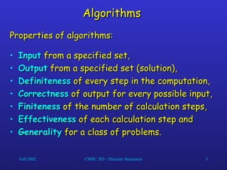
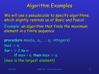
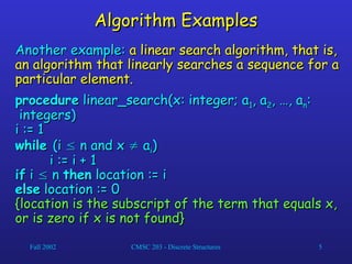
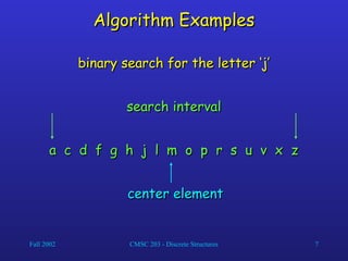
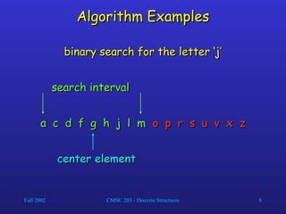
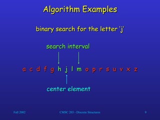
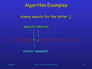
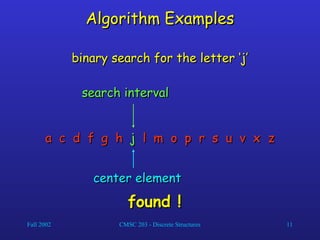
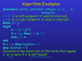
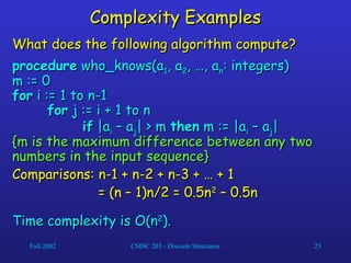
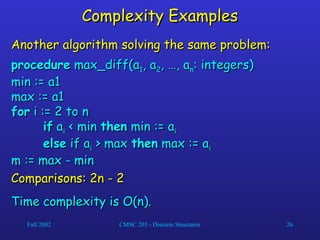
Fall 2002 CMSC 203 - Discrete Structures 1
Enough Mathematical Appetizers!
Let us look at something more interesting:
Algorithms
Algorithms
Fall 2002 CMSC 203 - Discrete Structures 2
Algorithms
Algorithms
What is an algorithm?
An algorithm is a finite set of precise instructions
for performing a computation or for solving a
problem.
problem.
This is a rather vague definition. You will get to
know a more precise and mathematically useful
definition when you attend CMSC441.
But this one is good enough for now…
Fall 2002 CMSC 203 - Discrete Structures 3
Algorithms
Algorithms
Properties of algorithms:
• Input
Input from a specified set,
from a specified set,
• Output
Output from a specified set (solution),
from a specified set (solution),
• Definiteness
Definiteness of every step in the computation,
of every step in the computation,
• Correctness
Correctness of output for every possible input,
of output for every possible input,
• Finiteness
Finiteness of the number of calculation steps,
of the number of calculation steps,
• Effectiveness
Effectiveness of each calculation step and
of each calculation step and
• Generality
Generality for a class of problems.
for a class of problems.
Fall 2002 CMSC 203 - Discrete Structures 4
Algorithm Examples
Algorithm Examples
We will use a pseudocode to specify algorithms,
which slightly reminds us of Basic and Pascal.
Example:
Example: an algorithm that finds the maximum
an algorithm that finds the maximum
element in a finite sequence
procedure
procedure max(a
max(a1
1, a
, a2
2, …, a
, …, an
n: integers)
: integers)
max := a
max := a1
1
for
for i := 2
i := 2 to
to n
n
if
if max < a
max < ai
i then
then max := a
max := ai
i
{max is the largest element}
Fall 2002 CMSC 203 - Discrete Structures 5
Algorithm Examples
Algorithm Examples
Another example:
Another example: a linear search algorithm, that is,
a linear search algorithm, that is,
an algorithm that linearly searches a sequence for a
particular element.
particular element.
procedure
procedure linear_search(x: integer; a
linear_search(x: integer; a1
1, a
, a2
2, …, a
, …, an
n:
:
integers)
integers)
i := 1
i := 1
while
while (i
(i 
 n and x
n and x 
 a
ai
i)
)
i := i + 1
i := i + 1
if
if i
i 
 n
n then
then location := i
location := i
else
else location := 0
location := 0
{location is the subscript of the term that equals x,
or is zero if x is not found}
Fall 2002 CMSC 203 - Discrete Structures 6
Algorithm Examples
Algorithm Examples
If the terms in a sequence are ordered, a binary
search algorithm is more efficient than linear
search.
search.
The binary search algorithm iteratively restricts
the relevant search interval until it closes in on
the position of the element to be located.
Fall 2002 CMSC 203 - Discrete Structures 7
Algorithm Examples
Algorithm Examples
a c d f g h j l m o p r s u v x z
binary search for the letter ‘j’
center element
center element
search interval
search interval
Fall 2002 CMSC 203 - Discrete Structures 8
Algorithm Examples
Algorithm Examples
a c d f g h j l m
a c d f g h j l m o p r s u v x z
o p r s u v x z
binary search for the letter ‘j’
center element
center element
search interval
search interval
Fall 2002 CMSC 203 - Discrete Structures 9
Algorithm Examples
Algorithm Examples
a c d f g
a c d f g h j l m
h j l m o p r s u v x z
o p r s u v x z
binary search for the letter ‘j’
center element
center element
search interval
search interval
Fall 2002 CMSC 203 - Discrete Structures 10
Algorithm Examples
Algorithm Examples
a c d f g
a c d f g h j
h j l m
l m o p r s u v x z
o p r s u v x z
binary search for the letter ‘j’
center element
center element
search interval
search interval
Fall 2002 CMSC 203 - Discrete Structures 11
Algorithm Examples
Algorithm Examples
a c d f g
a c d f g h
h j
j l m
l m o p r s u v x z
o p r s u v x z
binary search for the letter ‘j’
center element
center element
search interval
search interval
found !
found !
Fall 2002 CMSC 203 - Discrete Structures 12
Algorithm Examples
Algorithm Examples
procedure
procedure binary_search(x: integer; a
binary_search(x: integer; a1
1, a
, a2
2, …, a
, …, an
n:
:
integers)
integers)
i := 1
i := 1 {i is left endpoint of search interval}
{i is left endpoint of search interval}
j := n
j := n {j is right endpoint of search interval}
{j is right endpoint of search interval}
while
while (i < j)
(i < j)
begin
begin
m :=
m := 
(i + j)/2
(i + j)/2

if
if x > a
x > am
m then
then i := m + 1
i := m + 1
else
else j := m
j := m
end
end
if
if x = a
x = ai
i then
then location := i
location := i
else
else location := 0
location := 0
{location is the subscript of the term that equals
x, or is zero if x is not found}
Fall 2002 CMSC 203 - Discrete Structures 13
Complexity
Complexity
In general, we are not so much interested in the
time and space complexity for small inputs.
For example, while the difference in time
complexity between linear and binary search is
meaningless for a sequence with n = 10, it is
gigantic for n = 2
gigantic for n = 230
30
.
.
Fall 2002 CMSC 203 - Discrete Structures 14
Complexity
Complexity
For example, let us assume two algorithms A and
B that solve the same class of problems.
The time complexity of A is 5,000n, the one for
B is
B is 
1.1
1.1n
n

 for an input with n elements.
for an input with n elements.
For n = 10, A requires 50,000 steps, but B only 3,
so B seems to be superior to A.
For n = 1000, however, A requires 5,000,000
steps, while B requires 2.5
steps, while B requires 2.5
10
1041
41
steps.
steps.
Fall 2002 CMSC 203 - Discrete Structures 15
Complexity
Complexity
This means that algorithm B cannot be used for
large inputs, while algorithm A is still feasible.
So what is important is the
So what is important is the growth
growth of the
of the
complexity functions.
The growth of time and space complexity with
increasing input size n is a suitable measure for
the comparison of algorithms.
Fall 2002 CMSC 203 - Discrete Structures 16
Complexity
Complexity
Comparison:
Comparison: time complexity of algorithms A and B
time complexity of algorithms A and B
Algorithm A
Algorithm A Algorithm B
Algorithm B
Input Size
Input Size
n
n
10
10
100
100
1,000
1,000
1,000,000
1,000,000
5,000n
5,000n
50,000
50,000
500,000
500,000
5,000,000
5,000,000
5
5
10
109
9

1.1
1.1n
n


3
3
2.5
2.5
10
1041
41
13,781
13,781
4.8
4.8
10
1041392
41392
Fall 2002 CMSC 203 - Discrete Structures 17
The Growth of Functions
The growth of functions is usually described
using the
using the big-O notation
big-O notation.
.
Definition:
Definition: Let f and g be functions from the
Let f and g be functions from the
integers or the real numbers to the real numbers.
We say that f(x) is O(g(x)) if there are constants
C and k such that
C and k such that
|f(x)|
|f(x)| 
 C|g(x)|
C|g(x)|
whenever x > k.
whenever x > k.
Fall 2002 CMSC 203 - Discrete Structures 18
The Growth of Functions
When we analyze the growth of
When we analyze the growth of complexity
complexity
functions
functions, f(x) and g(x) are always positive.
, f(x) and g(x) are always positive.
Therefore, we can simplify the big-O requirement
to
to
f(x)
f(x) 
 C
C
g(x) whenever x > k.
g(x) whenever x > k.
If we want to show that f(x) is O(g(x)), we only
need to find
need to find one
one pair (C, k) (which is never unique).
pair (C, k) (which is never unique).
Fall 2002 CMSC 203 - Discrete Structures 19
The Growth of Functions
The idea behind the big-O notation is to establish
an
an upper boundary
upper boundary for the growth of a function
for the growth of a function
f(x) for
f(x) for large
large x.
x.
This boundary is specified by a function g(x) that
is usually much
is usually much simpler
simpler than f(x).
than f(x).
We accept the constant C in the requirement
f(x)
f(x) 
 C
C
g(x) whenever x > k,
g(x) whenever x > k,
because
because C does not grow with x.
C does not grow with x.
We are only interested in large x, so it is OK if
f(x) > C
f(x) > C
g(x) for x
g(x) for x 
 k.
k.
Fall 2002 CMSC 203 - Discrete Structures 20
The Growth of Functions
Example:
Example:
Show that f(x) = x
Show that f(x) = x2
2
+ 2x + 1 is O(x
+ 2x + 1 is O(x2
2
).
).
For x > 1 we have:
For x > 1 we have:
x
x2
2
+ 2x + 1
+ 2x + 1 
 x
x2
2
+ 2x
+ 2x2
2
+ x
+ x2
2

 x
x2
2
+ 2x + 1
+ 2x + 1 
 4x
4x2
2
Therefore, for C = 4 and k = 1:
f(x)
f(x) 
 Cx
Cx2
2
whenever x > k.
whenever x > k.

 f(x) is O(x
f(x) is O(x2
2
).
).
Fall 2002 CMSC 203 - Discrete Structures 21
The Growth of Functions
Question: If f(x) is O(x
Question: If f(x) is O(x2
2
), is it also O(x
), is it also O(x3
3
)?
)?
Yes.
Yes. x
x3
3
grows faster than x
grows faster than x2
2
, so x
, so x3
3
grows also
grows also
faster than f(x).
faster than f(x).
Therefore, we always have to find the
Therefore, we always have to find the smallest
smallest
simple function g(x) for which f(x) is O(g(x)).
Fall 2002 CMSC 203 - Discrete Structures 22
The Growth of Functions
“
“Popular” functions g(n) are
Popular” functions g(n) are
n log n, 1, 2
n log n, 1, 2n
n
, n
, n2
2
, n!, n, n
, n!, n, n3
3
, log n
, log n
Listed from slowest to fastest growth:
• 1
1
• log n
log n
• n
n
• n log n
n log n
• n
n2
2
• n
n3
3
• 2
2n
n
• n!
n!
Fall 2002 CMSC 203 - Discrete Structures 23
The Growth of Functions
A problem that can be solved with polynomial
worst-case complexity is called
worst-case complexity is called tractable
tractable.
.
Problems of higher complexity are called
intractable.
intractable.
Problems that no algorithm can solve are called
unsolvable
unsolvable.
.
You will find out more about this in CMSC441.
Fall 2002 CMSC 203 - Discrete Structures 24
Useful Rules for Big-O
For any
For any polynomial
polynomial f(x) = a
f(x) = an
nx
xn
n
+ a
+ an-1
n-1x
xn-1
n-1
+ … + a
+ … + a0
0, where
, where
a
a0
0, a
, a1
1, …, a
, …, an
n are real numbers,
are real numbers,
f(x) is O(x
f(x) is O(xn
n
).
).
If f
If f1
1(x) is O(g
(x) is O(g1
1(x)) and f
(x)) and f2
2(x) is O(g
(x) is O(g2
2(x)), then
(x)), then
(f
(f1
1 + f
+ f2
2)(x) is O(max(g
)(x) is O(max(g1
1(x), g
(x), g2
2(x)))
(x)))
If f
If f1
1(x) is O(g(x)) and f
(x) is O(g(x)) and f2
2(x) is O(g(x)), then
(x) is O(g(x)), then
(f
(f1
1 + f
+ f2
2)(x) is O(g(x)).
)(x) is O(g(x)).
If f
If f1
1(x) is O(g
(x) is O(g1
1(x)) and f
(x)) and f2
2(x) is O(g
(x) is O(g2
2(x)), then
(x)), then
(f
(f1
1f
f2
2)(x) is O(g
)(x) is O(g1
1(x) g
(x) g2
2(x)).
(x)).
Fall 2002 CMSC 203 - Discrete Structures 25
Complexity Examples
Complexity Examples
What does the following algorithm compute?
procedure
procedure who_knows(a
who_knows(a1
1, a
, a2
2, …, a
, …, an
n: integers)
: integers)
m := 0
m := 0
for
for i := 1 to n-1
i := 1 to n-1
for
for j := i + 1 to n
j := i + 1 to n
if
if |a
|ai
i – a
– aj
j| > m
| > m then
then m := |a
m := |ai
i – a
– aj
j|
|
{m is the maximum difference between any two
numbers in the input sequence}
Comparisons: n-1 + n-2 + n-3 + … + 1
= (n – 1)n/2 = 0.5n
= (n – 1)n/2 = 0.5n2
2
– 0.5n
– 0.5n
Time complexity is O(n
Time complexity is O(n2
2
).
).
Fall 2002 CMSC 203 - Discrete Structures 26
Complexity Examples
Complexity Examples
Another algorithm solving the same problem:
procedure
procedure max_diff(a
max_diff(a1
1, a
, a2
2, …, a
, …, an
n: integers)
: integers)
min := a1
min := a1
max := a1
max := a1
for
for i := 2 to n
i := 2 to n
if
if a
ai
i < min
< min then
then min := a
min := ai
i
else
else if a
if ai
i > max
> max then
then max := a
max := ai
i
m := max - min
m := max - min
Comparisons: 2n - 2
Comparisons: 2n - 2
Time complexity is O(n).
Fall 2002 CMSC 203 - Discrete Structures 27
Let us get into…
Let us get into…
Number Theory
Number Theory
Fall 2002 CMSC 203 - Discrete Structures 28
Introduction to Number Theory
Number theory is about
Number theory is about integers
integers and their
and their
properties.
properties.
We will start with the basic principles of
• divisibility,
divisibility,
• greatest common divisors,
greatest common divisors,
• least common multiples, and
least common multiples, and
• modular arithmetic
modular arithmetic
and look at some relevant algorithms.
Fall 2002 CMSC 203 - Discrete Structures 29
Division
Division
If a and b are integers with a
If a and b are integers with a 
 0, we say that
0, we say that
a
a divides
divides b if there is an integer c so that b = ac.
b if there is an integer c so that b = ac.
When a divides b we say that a is a
When a divides b we say that a is a factor
factor of b
of b
and that b is a
and that b is a multiple
multiple of a.
of a.
The notation
The notation a | b
a | b means that a divides b.
means that a divides b.
We write
We write a
a χ
χ b
b when a does not divide b
when a does not divide b
(see book for correct symbol).
Fall 2002 CMSC 203 - Discrete Structures 30
Divisibility Theorems
For integers a, b, and c it is true that
• if a | b and a | c, then a | (b + c)
if a | b and a | c, then a | (b + c)
Example:
Example: 3 | 6 and 3 | 9, so 3 | 15.
3 | 6 and 3 | 9, so 3 | 15.
• if a | b, then a | bc for all integers c
if a | b, then a | bc for all integers c
Example:
Example: 5 | 10, so 5 | 20, 5 | 30, 5 | 40, …
5 | 10, so 5 | 20, 5 | 30, 5 | 40, …
• if a | b and b | c, then a | c
if a | b and b | c, then a | c
Example:
Example: 4 | 8 and 8 | 24, so 4 | 24.
4 | 8 and 8 | 24, so 4 | 24.
Fall 2002 CMSC 203 - Discrete Structures 31
Primes
Primes
A positive integer p greater than 1 is called prime
if the only positive factors of p are 1 and p.
Note: 1 is not a prime
A positive integer that is greater than 1 and is not
prime is called composite.
The fundamental theorem of arithmetic:
Every positive integer can be written
Every positive integer can be written uniquely
uniquely as
as
the
the product of primes
product of primes, where the prime factors
, where the prime factors
are written in order of increasing size.
Fall 2002 CMSC 203 - Discrete Structures 32
Primes
Primes
Examples:
Examples:
3·5
3·5
48 =
48 =
17 =
17 =
100 =
100 =
512 =
512 =
515 =
515 =
28 =
28 =
15 =
15 =
2·2·2·2·3 = 2
2·2·2·2·3 = 24
4
·3
·3
17
17
2·2·5·5 = 2
2·2·5·5 = 22
2
·5
·52
2
2·2·2·2·2·2·2·2·2 = 2
2·2·2·2·2·2·2·2·2 = 29
9
5·103
5·103
2·2·7
2·2·7
Fall 2002 CMSC 203 - Discrete Structures 33
Primes
Primes
If n is a composite integer, then n has a prime
divisor less than or equal .
This is easy to see: if n is a composite integer, it
must have at least two prime divisors. Let the
largest two be p
largest two be p1
1 and p
and p2
2. Then p
. Then p1
1
p
p2
2 <= n.
<= n.
p
p1
1 and p
and p2
2 cannot both be greater than
cannot both be greater than
, because then p
, because then p1
1
p
p2
2 > n.
> n.
n
n
Fall 2002 CMSC 203 - Discrete Structures 34
The Division Algorithm
Let
Let a
a be an integer and
be an integer and d
d a positive integer.
a positive integer.
Then there are unique integers
Then there are unique integers q
q and
and r
r, with
, with
0
0 
 r < d
r < d, such that
, such that a = dq + r
a = dq + r.
.
In the above equation,
• d
d is called the divisor,
is called the divisor,
• a
a is called the dividend,
is called the dividend,
• q
q is called the quotient, and
is called the quotient, and
• r
r is called the remainder.
is called the remainder.
Fall 2002 CMSC 203 - Discrete Structures 35
The Division Algorithm
Example:
Example:
When we divide 17 by 5, we have
17 = 5
17 = 5
3 + 2.
3 + 2.
• 17 is the dividend,
17 is the dividend,
• 5 is the divisor,
5 is the divisor,
• 3 is called the quotient, and
3 is called the quotient, and
• 2 is called the remainder.
2 is called the remainder.
Fall 2002 CMSC 203 - Discrete Structures 36
The Division Algorithm
Another example:
Another example:
What happens when we divide -11 by 3 ?
Note that the remainder cannot be negative.
-11 = 3
-11 = 3
(-4) + 1.
(-4) + 1.
• -11 is the dividend,
-11 is the dividend,
• 3 is the divisor,
3 is the divisor,
• -4 is called the quotient, and
-4 is called the quotient, and
• 1 is called the remainder.
1 is called the remainder.
Fall 2002 CMSC 203 - Discrete Structures 37
Greatest Common Divisors
Let a and b be integers, not both zero.
The largest integer d such that d | a and d | b is
called the
called the greatest common divisor
greatest common divisor of a and b.
of a and b.
The greatest common divisor of a and b is denoted
by gcd(a, b).
by gcd(a, b).
Example 1:
Example 1: What is gcd(48, 72) ?
What is gcd(48, 72) ?
The positive common divisors of 48 and 72 are
1, 2, 3, 4, 6, 8, 12, 16, and 24, so gcd(48, 72) = 24.
Example 2:
Example 2: What is gcd(19, 72) ?
What is gcd(19, 72) ?
The only positive common divisor of 19 and 72 is
1, so gcd(19, 72) = 1.
Fall 2002 CMSC 203 - Discrete Structures 38
Greatest Common Divisors
Using prime factorizations:
a = p
a = p1
1
a
a
1
1 p
p2
2
a
a
2
2 … p
… pn
n
a
a
n
n , b = p
, b = p1
1
b
b
1
1 p
p2
2
b
b
2
2 … p
… pn
n
b
b
n
n ,
,
where p
where p1
1 < p
< p2
2 < … < p
< … < pn
n and a
and ai
i, b
, bi
i 
 N
N for 1
for 1 
 i
i 
 n
n
gcd(a, b) = p
gcd(a, b) = p1
1
min(a
min(a
1
1, b
, b
1
1 )
)
p
p2
2
min(a
min(a
2
2, b
, b
2
2 )
)
… p
… pn
n
min(a
min(a
n
n, b
, b
n
n )
)
Example:
Example:
a = 60 =
a = 60 = 2
22
2
3
31
1
5
51
1
b = 54 =
b = 54 = 2
21
1
3
33
3
5
50
0
gcd(a, b) =
gcd(a, b) = 2
21
1
3
31
1
5
50
0
= 6
= 6
Fall 2002 CMSC 203 - Discrete Structures 39
Relatively Prime Integers
Definition:
Definition:
Two integers a and b are
Two integers a and b are relatively prime
relatively prime if
if
gcd(a, b) = 1.
gcd(a, b) = 1.
Examples:
Examples:
Are 15 and 28 relatively prime?
Yes, gcd(15, 28) = 1.
Are 55 and 28 relatively prime?
Yes, gcd(55, 28) = 1.
Are 35 and 28 relatively prime?
No, gcd(35, 28) = 7.
Fall 2002 CMSC 203 - Discrete Structures 40
Relatively Prime Integers
Definition:
Definition:
The integers a
The integers a1
1, a
, a2
2, …, a
, …, an
n are
are pairwise relatively
pairwise relatively
prime
prime if gcd(a
if gcd(ai
i, a
, aj
j) = 1 whenever 1
) = 1 whenever 1 
 i < j
i < j 
 n.
n.
Examples:
Examples:
Are 15, 17, and 27 pairwise relatively prime?
No, because gcd(15, 27) = 3.
Are 15, 17, and 28 pairwise relatively prime?
Yes, because gcd(15, 17) = 1, gcd(15, 28) = 1 and
gcd(17, 28) = 1.
gcd(17, 28) = 1.
Fall 2002 CMSC 203 - Discrete Structures 41
Least Common Multiples
Definition:
Definition:
The
The least common multiple
least common multiple of the positive
of the positive
integers a and b is the smallest positive integer
that is divisible by both a and b.
We denote the least common multiple of a and b
by lcm(a, b).
by lcm(a, b).
Examples:
Examples:
lcm(3, 7) =
lcm(3, 7) = 21
21
lcm(4, 6) =
lcm(4, 6) = 12
12
lcm(5, 10) =
lcm(5, 10) = 10
10
Fall 2002 CMSC 203 - Discrete Structures 42
Least Common Multiples
Using prime factorizations:
a = p
a = p1
1
a
a
1
1 p
p2
2
a
a
2
2 … p
… pn
n
a
a
n
n , b = p
, b = p1
1
b
b
1
1 p
p2
2
b
b
2
2 … p
… pn
n
b
b
n
n ,
,
where p
where p1
1 < p
< p2
2 < … < p
< … < pn
n and a
and ai
i, b
, bi
i 
 N
N for 1
for 1 
 i
i 
 n
n
lcm(a, b) = p
lcm(a, b) = p1
1
max(a
max(a
1
1, b
, b
1
1 )
)
p
p2
2
max(a
max(a
2
2, b
, b
2
2 )
)
… p
… pn
n
max(a
max(a
n
n, b
, b
n
n )
)
Example:
Example:
a = 60 =
a = 60 = 2
22
2
3
31
1
5
51
1
b = 54 =
b = 54 = 2
21
1
3
33
3
5
50
0
lcm(a, b) =
lcm(a, b) = 2
22
2
3
33
3
5
51
1
= 4
= 4
27
27
5 = 540
5 = 540
Fall 2002 CMSC 203 - Discrete Structures 43
GCD and LCM
GCD and LCM
a = 60 =
a = 60 = 2
22
2
3
31
1
5
51
1
b = 54 =
b = 54 = 2
21
1
3
33
3
5
50
0
lcm(a, b) =
lcm(a, b) = 2
22
2
3
33
3
5
51
1
= 540
= 540
gcd(a, b) =
gcd(a, b) = 2
21
1
3
31
1
5
50
0
= 6
= 6
Theorem: a
Theorem: a
b =
b = gcd(a,b)
gcd(a,b)
lcm(a,b)
lcm(a,b)
Fall 2002 CMSC 203 - Discrete Structures 44
Modular Arithmetic
Modular Arithmetic
Let a be an integer and m be a positive integer.
We denote by
We denote by a mod m
a mod m the remainder when a is
the remainder when a is
divided by m.
divided by m.
Examples:
Examples:
9 mod 4 =
9 mod 4 = 1
1
9 mod 3 =
9 mod 3 = 0
0
9 mod 10 =
9 mod 10 = 9
9
-13 mod 4 =
-13 mod 4 = 3
3
Fall 2002 CMSC 203 - Discrete Structures 45
Congruences
Congruences
Let a and b be integers and m be a positive integer.
We say that
We say that a is congruent to b modulo m
a is congruent to b modulo m if
if
m divides a – b.
m divides a – b.
We use the notation
We use the notation a
a 
 b (mod m)
b (mod m) to indicate
to indicate
that a is congruent to b modulo m.
In other words:
In other words:
a
a 
 b (mod m) if and only if
b (mod m) if and only if a mod m = b mod m
a mod m = b mod m.
.
Fall 2002 CMSC 203 - Discrete Structures 46
Congruences
Congruences
Examples:
Examples:
Is it true that 46
Is it true that 46 
 68 (mod 11) ?
68 (mod 11) ?
Yes, because 11 | (46 – 68).
Is it true that 46
Is it true that 46 
 68 (mod 22)?
68 (mod 22)?
Yes, because 22 | (46 – 68).
For which integers z is it true that z
For which integers z is it true that z 
 12 (mod 10)?
12 (mod 10)?
It is true for any z
It is true for any z
{…,-28, -18, -8, 2, 12, 22, 32, …}
{…,-28, -18, -8, 2, 12, 22, 32, …}
Theorem:
Theorem: Let m be a positive integer. The integers
Let m be a positive integer. The integers
a and b are congruent modulo m if and only if there
is an integer k such that a = b + km.
Fall 2002 CMSC 203 - Discrete Structures 47
Congruences
Congruences
Theorem:
Theorem: Let m be a positive integer.
Let m be a positive integer.
If a
If a 
 b (mod m) and c
b (mod m) and c 
 d (mod m), then
d (mod m), then
a + c
a + c 
 b + d (mod m) and ac
b + d (mod m) and ac 
 bd (mod m).
bd (mod m).
Proof:
Proof:
We know that a
We know that a 
 b (mod m) and c
b (mod m) and c 
 d (mod m)
d (mod m)
implies that there are integers s and t with
b = a + sm and d = c + tm.
Therefore,
Therefore,
b + d = (a + sm) + (c + tm) = (a + c) + m(s + t) and
bd = (a + sm)(c + tm) = ac + m(at + cs + stm).
Hence, a + c
Hence, a + c 
 b + d (mod m) and ac
b + d (mod m) and ac 
 bd (mod m).
bd (mod m).
Fall 2002 CMSC 203 - Discrete Structures 48
Congruences
Congruences
Theorem:
Theorem: Let m be a positive integer. a
Let m be a positive integer. a 
 b (mod m)
b (mod m)
iff a mod m = b mod m.
Proof:
Proof:
Let a = mq1 + r1, and b = mq2 + r2.
Only if part:
Only if part: a mod m = b mod m
a mod m = b mod m 
 r1 = r2, therefore
r1 = r2, therefore
a – b = m(q1 – q2), and a
a – b = m(q1 – q2), and a 
 b (mod m).
b (mod m).
If part:
If part: a
a 
 b (mod m) implies
b (mod m) implies
a – b = mq
a – b = mq
mq1 + r1 – (mq2 + r2) = mq
r1 – r2 = m(q – q1 + q2).
Since 0
Since 0 
 r1, r2
r1, r2 
 m, 0
m, 0 
 |r1 - r2|
|r1 - r2| 
 m. The only
m. The only
multiple in that range is 0.
Therefore r1 = r2, and a mod m = b mod m.
Fall 2002 CMSC 203 - Discrete Structures 49
The Euclidean Algorithm
The
The Euclidean Algorithm
Euclidean Algorithm finds the
finds the greatest
greatest
common divisor
common divisor of two integers a and b.
of two integers a and b.
For example, if we want to find gcd(287, 91), we
divide
divide 287 by 91:
287 by 91:
287 = 91
287 = 91
3 + 14
3 + 14
We know that for integers a, b and c,
if a | b and a | c, then a | (b + c).
Therefore, any divisor (including their gcd) of 287
and 91 must also be a divisor of 287 - 91
and 91 must also be a divisor of 287 - 91
3 = 14.
3 = 14.
Consequently, gcd(287, 91) = gcd(14, 91).
Fall 2002 CMSC 203 - Discrete Structures 50
The Euclidean Algorithm
In the next step, we divide 91 by 14:
91 = 14
91 = 14
6 + 7
6 + 7
This means that gcd(14, 91) = gcd(14, 7).
So we divide 14 by 7:
14 = 7
14 = 7
2 + 0
2 + 0
We find that 7 | 14, and thus gcd(14, 7) = 7.
Therefore, gcd(287, 91) = 7.
Fall 2002 CMSC 203 - Discrete Structures 51
The Euclidean Algorithm
In
In pseudocode
pseudocode, the algorithm can be implemented
, the algorithm can be implemented
as follows:
as follows:
procedure
procedure gcd(a, b: positive integers)
gcd(a, b: positive integers)
x := a
x := a
y := b
y := b
while
while y
y 
 0
0
begin
begin
r := x
r := x mod
mod y
y
x := y
x := y
y := r
y := r
end
end {x is gcd(a, b)}
{x is gcd(a, b)}
Fall 2002 CMSC 203 - Discrete Structures 52
Representations of Integers
Let b be a positive integer greater than 1.
Then if n is a positive integer, it can be expressed
uniquely
uniquely in the form:
in the form:
n = a
n = ak
kb
bk
k
+ a
+ ak-1
k-1b
bk-1
k-1
+ … + a
+ … + a1
1b + a
b + a0
0,
,
where k is a nonnegative integer,
a
a0
0, a
, a1
1, …, a
, …, ak
k are nonnegative integers less than b,
are nonnegative integers less than b,
and a
and ak
k 
 0.
0.
Example for b=10:
Example for b=10:
859 = 8
859 = 8
10
102
2
+ 5
+ 5
10
101
1
+ 9
+ 9
10
100
0
Fall 2002 CMSC 203 - Discrete Structures 53
Representations of Integers
Example for b=2 (binary expansion):
(10110)
(10110)2
2 = 1
= 1
2
24
4
+ 1
+ 1
2
22
2
+ 1
+ 1
2
21
1
= (22)
= (22)10
10
Example for b=16 (hexadecimal expansion):
(we use letters A to F to indicate numbers 10 to 15)
(3A0F)
(3A0F)16
16 = 3
= 3
16
163
3
+ 10
+ 10
16
162
2
+ 15
+ 15
16
160
0
= (14863)
= (14863)10
10
Fall 2002 CMSC 203 - Discrete Structures 54
Representations of Integers
How can we construct the base b expansion of an
integer n?
integer n?
First, divide n by b to obtain a quotient q
First, divide n by b to obtain a quotient q0
0 and
and
remainder a
remainder a0
0, that is,
, that is,
n = bq
n = bq0
0 + a
+ a0
0, where 0
, where 0 
 a
a0
0 < b.
< b.
The remainder a
The remainder a0
0 is the rightmost digit in the base b
is the rightmost digit in the base b
expansion of n.
expansion of n.
Next, divide q
Next, divide q0
0 by b to obtain:
by b to obtain:
q
q0
0 = bq
= bq1
1 + a
+ a1
1, where 0
, where 0 
 a
a1
1 < b.
< b.
a
a1
1 is the second digit from the right in the base b
is the second digit from the right in the base b
expansion of n. Continue this process until you obtain a
quotient equal to zero.
Fall 2002 CMSC 203 - Discrete Structures 55
Representations of Integers
Example:
Example:
What is the base 8 expansion of (12345)
What is the base 8 expansion of (12345)10
10 ?
?
First, divide 12345 by 8:
12345 = 8
12345 = 8
1543 + 1
1543 + 1
1543 = 8
1543 = 8
192 + 7
192 + 7
192 = 8
192 = 8
24 + 0
24 + 0
24 = 8
24 = 8
3 + 0
3 + 0
3 = 8
3 = 8
0 + 3
0 + 3
The result is: (12345)
The result is: (12345)10
10 = (30071)
= (30071)8
8.
.
Fall 2002 CMSC 203 - Discrete Structures 56
Representations of Integers
procedure
procedure base_b_expansion(n, b: positive integers)
base_b_expansion(n, b: positive integers)
q := n
q := n
k := 0
k := 0
while
while q
q 
 0
0
begin
begin
a
ak
k := q mod b
:= q mod b
q :=
q := 
q/b
q/b

k := k + 1
k := k + 1
end
end
{the base b expansion of n is (a
{the base b expansion of n is (ak-1
k-1 … a
… a1
1a
a0
0)
)b
b }
}
Fall 2002 CMSC 203 - Discrete Structures 57
Addition of Integers
How do we (humans) add two integers?
Example:
Example: 7583
7583
+
+ 4932
4932
5
5
1
1
5
5
2
2
1
1
1
1
1
1
1
1 carry
carry
Binary expansions:
Binary expansions: (1011)
(1011)2
2
+
+ (1010)
(1010)2
2
1
1
0
0
carry
carry
1
1
1
1
0
0
1
1
1
1
(
( )
)2
2
Fall 2002 CMSC 203 - Discrete Structures 58
Addition of Integers
Let a = (a
Let a = (an-1
n-1a
an-2
n-2…a
…a1
1a
a0
0)
)2
2, b = (b
, b = (bn-1
n-1b
bn-2
n-2…b
…b1
1b
b0
0)
)2.
2.
How can we
How can we algorithmically
algorithmically add these two binary
add these two binary
numbers?
numbers?
First, add their rightmost bits:
a
a0
0 + b
+ b0
0 = c
= c0
0
2 + s
2 + s0
0,
,
where s
where s0
0 is the
is the rightmost bit
rightmost bit in the binary expansion
in the binary expansion
of a + b, and c
of a + b, and c0
0 is the
is the carry
carry.
.
Then, add the next pair of bits and the carry:
a
a1
1 + b
+ b1
1 + c
+ c0
0 = c
= c1
1
2 + s
2 + s1
1,
,
where s
where s1
1 is the
is the next bit
next bit in the binary expansion of a +
in the binary expansion of a +
b, and c
b, and c1
1 is the carry.
is the carry.
Fall 2002 CMSC 203 - Discrete Structures 59
Addition of Integers
Continue this process until you obtain c
Continue this process until you obtain cn-1
n-1.
.
The leading bit of the sum is s
The leading bit of the sum is sn
n = c
= cn-1
n-1.
.
The result is:
The result is:
a + b = (s
a + b = (sn
ns
sn-1
n-1…s
…s1
1s
s0
0)
)2
2
Fall 2002 CMSC 203 - Discrete Structures 60
Addition of Integers
Example:
Example:
Add a = (1110)
Add a = (1110)2
2 and b = (1011)
and b = (1011)2
2.
.
a
a0
0 + b
+ b0
0 = 0 + 1 = 0
= 0 + 1 = 0
2 + 1, so that c
2 + 1, so that c0
0 = 0 and s
= 0 and s0
0 = 1.
= 1.
a
a1
1 + b
+ b1
1 + c
+ c0
0 = 1 + 1 + 0 = 1
= 1 + 1 + 0 = 1
2 + 0, so c
2 + 0, so c1
1 = 1 and s
= 1 and s1
1 = 0.
= 0.
a
a2
2 + b
+ b2
2 + c
+ c1
1 = 1 + 0 + 1 = 1
= 1 + 0 + 1 = 1
2 + 0, so c
2 + 0, so c2
2 = 1 and s
= 1 and s2
2 = 0.
= 0.
a
a3
3 + b
+ b3
3 + c
+ c2
2 = 1 + 1 + 1 = 1
= 1 + 1 + 1 = 1
2 + 1, so c
2 + 1, so c3
3 = 1 and s
= 1 and s3
3 = 1.
= 1.
s
s4
4 = c
= c3
3 = 1.
= 1.
Therefore, s = a + b = (11001)
Therefore, s = a + b = (11001)2
2.
.
Fall 2002 CMSC 203 - Discrete Structures 61
Addition of Integers
procedure
procedure add(a, b: positive integers)
add(a, b: positive integers)
c := 0
c := 0
for j := 0 to n-1
for j := 0 to n-1
begin
begin
d :=
d := 
(a
(aj
j + b
+ bj
j + c)/2
+ c)/2

s
sj
j := a
:= aj
j + b
+ bj
j + c – 2d
+ c – 2d
c := d
c := d
end
end
s
sn
n := c
:= c
{the binary expansion of the sum is (s
{the binary expansion of the sum is (sn
ns
sn-1
n-1…s
…s1
1s
s0
0)
)2
2}
}

Ch02 algorithm 127836129812y12y823873893.ppt

  • 1.
    Fall 2002 CMSC203 - Discrete Structures 1 Enough Mathematical Appetizers! Enough Mathematical Appetizers! Let us look at something more interesting: Let us look at something more interesting: Algorithms Algorithms
  • 2.
    Fall 2002 CMSC203 - Discrete Structures 2 Algorithms Algorithms What is an algorithm? What is an algorithm? An algorithm is a finite set of precise instructions An algorithm is a finite set of precise instructions for performing a computation or for solving a for performing a computation or for solving a problem. problem. This is a rather vague definition. You will get to This is a rather vague definition. You will get to know a more precise and mathematically useful know a more precise and mathematically useful definition when you attend CMSC441. definition when you attend CMSC441. But this one is good enough for now… But this one is good enough for now…
  • 3.
    Fall 2002 CMSC203 - Discrete Structures 3 Algorithms Algorithms Properties of algorithms: Properties of algorithms: • Input Input from a specified set, from a specified set, • Output Output from a specified set (solution), from a specified set (solution), • Definiteness Definiteness of every step in the computation, of every step in the computation, • Correctness Correctness of output for every possible input, of output for every possible input, • Finiteness Finiteness of the number of calculation steps, of the number of calculation steps, • Effectiveness Effectiveness of each calculation step and of each calculation step and • Generality Generality for a class of problems. for a class of problems.
  • 4.
    Fall 2002 CMSC203 - Discrete Structures 4 Algorithm Examples Algorithm Examples We will use a pseudocode to specify algorithms, We will use a pseudocode to specify algorithms, which slightly reminds us of Basic and Pascal. which slightly reminds us of Basic and Pascal. Example: Example: an algorithm that finds the maximum an algorithm that finds the maximum element in a finite sequence element in a finite sequence procedure procedure max(a max(a1 1, a , a2 2, …, a , …, an n: integers) : integers) max := a max := a1 1 for for i := 2 i := 2 to to n n if if max < a max < ai i then then max := a max := ai i {max is the largest element} {max is the largest element}
  • 5.
    Fall 2002 CMSC203 - Discrete Structures 5 Algorithm Examples Algorithm Examples Another example: Another example: a linear search algorithm, that is, a linear search algorithm, that is, an algorithm that linearly searches a sequence for a an algorithm that linearly searches a sequence for a particular element. particular element. procedure procedure linear_search(x: integer; a linear_search(x: integer; a1 1, a , a2 2, …, a , …, an n: : integers) integers) i := 1 i := 1 while while (i (i   n and x n and x   a ai i) ) i := i + 1 i := i + 1 if if i i   n n then then location := i location := i else else location := 0 location := 0 {location is the subscript of the term that equals x, {location is the subscript of the term that equals x, or is zero if x is not found} or is zero if x is not found}
  • 6.
    Fall 2002 CMSC203 - Discrete Structures 6 Algorithm Examples Algorithm Examples If the terms in a sequence are ordered, a binary If the terms in a sequence are ordered, a binary search algorithm is more efficient than linear search algorithm is more efficient than linear search. search. The binary search algorithm iteratively restricts The binary search algorithm iteratively restricts the relevant search interval until it closes in on the relevant search interval until it closes in on the position of the element to be located. the position of the element to be located.
  • 7.
    Fall 2002 CMSC203 - Discrete Structures 7 Algorithm Examples Algorithm Examples a c d f g h j l m o p r s u v x z a c d f g h j l m o p r s u v x z binary search for the letter ‘j’ binary search for the letter ‘j’ center element center element search interval search interval
  • 8.
    Fall 2002 CMSC203 - Discrete Structures 8 Algorithm Examples Algorithm Examples a c d f g h j l m a c d f g h j l m o p r s u v x z o p r s u v x z binary search for the letter ‘j’ binary search for the letter ‘j’ center element center element search interval search interval
  • 9.
    Fall 2002 CMSC203 - Discrete Structures 9 Algorithm Examples Algorithm Examples a c d f g a c d f g h j l m h j l m o p r s u v x z o p r s u v x z binary search for the letter ‘j’ binary search for the letter ‘j’ center element center element search interval search interval
  • 10.
    Fall 2002 CMSC203 - Discrete Structures 10 Algorithm Examples Algorithm Examples a c d f g a c d f g h j h j l m l m o p r s u v x z o p r s u v x z binary search for the letter ‘j’ binary search for the letter ‘j’ center element center element search interval search interval
  • 11.
    Fall 2002 CMSC203 - Discrete Structures 11 Algorithm Examples Algorithm Examples a c d f g a c d f g h h j j l m l m o p r s u v x z o p r s u v x z binary search for the letter ‘j’ binary search for the letter ‘j’ center element center element search interval search interval found ! found !
  • 12.
    Fall 2002 CMSC203 - Discrete Structures 12 Algorithm Examples Algorithm Examples procedure procedure binary_search(x: integer; a binary_search(x: integer; a1 1, a , a2 2, …, a , …, an n: : integers) integers) i := 1 i := 1 {i is left endpoint of search interval} {i is left endpoint of search interval} j := n j := n {j is right endpoint of search interval} {j is right endpoint of search interval} while while (i < j) (i < j) begin begin m := m :=  (i + j)/2 (i + j)/2  if if x > a x > am m then then i := m + 1 i := m + 1 else else j := m j := m end end if if x = a x = ai i then then location := i location := i else else location := 0 location := 0 {location is the subscript of the term that equals {location is the subscript of the term that equals x, or is zero if x is not found} x, or is zero if x is not found}
  • 13.
    Fall 2002 CMSC203 - Discrete Structures 13 Complexity Complexity In general, we are not so much interested in the In general, we are not so much interested in the time and space complexity for small inputs. time and space complexity for small inputs. For example, while the difference in time For example, while the difference in time complexity between linear and binary search is complexity between linear and binary search is meaningless for a sequence with n = 10, it is meaningless for a sequence with n = 10, it is gigantic for n = 2 gigantic for n = 230 30 . .
  • 14.
    Fall 2002 CMSC203 - Discrete Structures 14 Complexity Complexity For example, let us assume two algorithms A and For example, let us assume two algorithms A and B that solve the same class of problems. B that solve the same class of problems. The time complexity of A is 5,000n, the one for The time complexity of A is 5,000n, the one for B is B is  1.1 1.1n n   for an input with n elements. for an input with n elements. For n = 10, A requires 50,000 steps, but B only 3, For n = 10, A requires 50,000 steps, but B only 3, so B seems to be superior to A. so B seems to be superior to A. For n = 1000, however, A requires 5,000,000 For n = 1000, however, A requires 5,000,000 steps, while B requires 2.5 steps, while B requires 2.5 10 1041 41 steps. steps.
  • 15.
    Fall 2002 CMSC203 - Discrete Structures 15 Complexity Complexity This means that algorithm B cannot be used for This means that algorithm B cannot be used for large inputs, while algorithm A is still feasible. large inputs, while algorithm A is still feasible. So what is important is the So what is important is the growth growth of the of the complexity functions. complexity functions. The growth of time and space complexity with The growth of time and space complexity with increasing input size n is a suitable measure for increasing input size n is a suitable measure for the comparison of algorithms. the comparison of algorithms.
  • 16.
    Fall 2002 CMSC203 - Discrete Structures 16 Complexity Complexity Comparison: Comparison: time complexity of algorithms A and B time complexity of algorithms A and B Algorithm A Algorithm A Algorithm B Algorithm B Input Size Input Size n n 10 10 100 100 1,000 1,000 1,000,000 1,000,000 5,000n 5,000n 50,000 50,000 500,000 500,000 5,000,000 5,000,000 5 5 10 109 9  1.1 1.1n n   3 3 2.5 2.5 10 1041 41 13,781 13,781 4.8 4.8 10 1041392 41392
  • 17.
    Fall 2002 CMSC203 - Discrete Structures 17 The Growth of Functions The Growth of Functions The growth of functions is usually described The growth of functions is usually described using the using the big-O notation big-O notation. . Definition: Definition: Let f and g be functions from the Let f and g be functions from the integers or the real numbers to the real numbers. integers or the real numbers to the real numbers. We say that f(x) is O(g(x)) if there are constants We say that f(x) is O(g(x)) if there are constants C and k such that C and k such that |f(x)| |f(x)|   C|g(x)| C|g(x)| whenever x > k. whenever x > k.
  • 18.
    Fall 2002 CMSC203 - Discrete Structures 18 The Growth of Functions The Growth of Functions When we analyze the growth of When we analyze the growth of complexity complexity functions functions, f(x) and g(x) are always positive. , f(x) and g(x) are always positive. Therefore, we can simplify the big-O requirement Therefore, we can simplify the big-O requirement to to f(x) f(x)   C C g(x) whenever x > k. g(x) whenever x > k. If we want to show that f(x) is O(g(x)), we only If we want to show that f(x) is O(g(x)), we only need to find need to find one one pair (C, k) (which is never unique). pair (C, k) (which is never unique).
  • 19.
    Fall 2002 CMSC203 - Discrete Structures 19 The Growth of Functions The Growth of Functions The idea behind the big-O notation is to establish The idea behind the big-O notation is to establish an an upper boundary upper boundary for the growth of a function for the growth of a function f(x) for f(x) for large large x. x. This boundary is specified by a function g(x) that This boundary is specified by a function g(x) that is usually much is usually much simpler simpler than f(x). than f(x). We accept the constant C in the requirement We accept the constant C in the requirement f(x) f(x)   C C g(x) whenever x > k, g(x) whenever x > k, because because C does not grow with x. C does not grow with x. We are only interested in large x, so it is OK if We are only interested in large x, so it is OK if f(x) > C f(x) > C g(x) for x g(x) for x   k. k.
  • 20.
    Fall 2002 CMSC203 - Discrete Structures 20 The Growth of Functions The Growth of Functions Example: Example: Show that f(x) = x Show that f(x) = x2 2 + 2x + 1 is O(x + 2x + 1 is O(x2 2 ). ). For x > 1 we have: For x > 1 we have: x x2 2 + 2x + 1 + 2x + 1   x x2 2 + 2x + 2x2 2 + x + x2 2   x x2 2 + 2x + 1 + 2x + 1   4x 4x2 2 Therefore, for C = 4 and k = 1: Therefore, for C = 4 and k = 1: f(x) f(x)   Cx Cx2 2 whenever x > k. whenever x > k.   f(x) is O(x f(x) is O(x2 2 ). ).
  • 21.
    Fall 2002 CMSC203 - Discrete Structures 21 The Growth of Functions The Growth of Functions Question: If f(x) is O(x Question: If f(x) is O(x2 2 ), is it also O(x ), is it also O(x3 3 )? )? Yes. Yes. x x3 3 grows faster than x grows faster than x2 2 , so x , so x3 3 grows also grows also faster than f(x). faster than f(x). Therefore, we always have to find the Therefore, we always have to find the smallest smallest simple function g(x) for which f(x) is O(g(x)). simple function g(x) for which f(x) is O(g(x)).
  • 22.
    Fall 2002 CMSC203 - Discrete Structures 22 The Growth of Functions The Growth of Functions “ “Popular” functions g(n) are Popular” functions g(n) are n log n, 1, 2 n log n, 1, 2n n , n , n2 2 , n!, n, n , n!, n, n3 3 , log n , log n Listed from slowest to fastest growth: Listed from slowest to fastest growth: • 1 1 • log n log n • n n • n log n n log n • n n2 2 • n n3 3 • 2 2n n • n! n!
  • 23.
    Fall 2002 CMSC203 - Discrete Structures 23 The Growth of Functions The Growth of Functions A problem that can be solved with polynomial A problem that can be solved with polynomial worst-case complexity is called worst-case complexity is called tractable tractable. . Problems of higher complexity are called Problems of higher complexity are called intractable. intractable. Problems that no algorithm can solve are called Problems that no algorithm can solve are called unsolvable unsolvable. . You will find out more about this in CMSC441. You will find out more about this in CMSC441.
  • 24.
    Fall 2002 CMSC203 - Discrete Structures 24 Useful Rules for Big-O Useful Rules for Big-O For any For any polynomial polynomial f(x) = a f(x) = an nx xn n + a + an-1 n-1x xn-1 n-1 + … + a + … + a0 0, where , where a a0 0, a , a1 1, …, a , …, an n are real numbers, are real numbers, f(x) is O(x f(x) is O(xn n ). ). If f If f1 1(x) is O(g (x) is O(g1 1(x)) and f (x)) and f2 2(x) is O(g (x) is O(g2 2(x)), then (x)), then (f (f1 1 + f + f2 2)(x) is O(max(g )(x) is O(max(g1 1(x), g (x), g2 2(x))) (x))) If f If f1 1(x) is O(g(x)) and f (x) is O(g(x)) and f2 2(x) is O(g(x)), then (x) is O(g(x)), then (f (f1 1 + f + f2 2)(x) is O(g(x)). )(x) is O(g(x)). If f If f1 1(x) is O(g (x) is O(g1 1(x)) and f (x)) and f2 2(x) is O(g (x) is O(g2 2(x)), then (x)), then (f (f1 1f f2 2)(x) is O(g )(x) is O(g1 1(x) g (x) g2 2(x)). (x)).
  • 25.
    Fall 2002 CMSC203 - Discrete Structures 25 Complexity Examples Complexity Examples What does the following algorithm compute? What does the following algorithm compute? procedure procedure who_knows(a who_knows(a1 1, a , a2 2, …, a , …, an n: integers) : integers) m := 0 m := 0 for for i := 1 to n-1 i := 1 to n-1 for for j := i + 1 to n j := i + 1 to n if if |a |ai i – a – aj j| > m | > m then then m := |a m := |ai i – a – aj j| | {m is the maximum difference between any two {m is the maximum difference between any two numbers in the input sequence} numbers in the input sequence} Comparisons: n-1 + n-2 + n-3 + … + 1 Comparisons: n-1 + n-2 + n-3 + … + 1 = (n – 1)n/2 = 0.5n = (n – 1)n/2 = 0.5n2 2 – 0.5n – 0.5n Time complexity is O(n Time complexity is O(n2 2 ). ).
  • 26.
    Fall 2002 CMSC203 - Discrete Structures 26 Complexity Examples Complexity Examples Another algorithm solving the same problem: Another algorithm solving the same problem: procedure procedure max_diff(a max_diff(a1 1, a , a2 2, …, a , …, an n: integers) : integers) min := a1 min := a1 max := a1 max := a1 for for i := 2 to n i := 2 to n if if a ai i < min < min then then min := a min := ai i else else if a if ai i > max > max then then max := a max := ai i m := max - min m := max - min Comparisons: 2n - 2 Comparisons: 2n - 2 Time complexity is O(n). Time complexity is O(n).
  • 27.
    Fall 2002 CMSC203 - Discrete Structures 27 Let us get into… Let us get into… Number Theory Number Theory
  • 28.
    Fall 2002 CMSC203 - Discrete Structures 28 Introduction to Number Theory Introduction to Number Theory Number theory is about Number theory is about integers integers and their and their properties. properties. We will start with the basic principles of We will start with the basic principles of • divisibility, divisibility, • greatest common divisors, greatest common divisors, • least common multiples, and least common multiples, and • modular arithmetic modular arithmetic and look at some relevant algorithms. and look at some relevant algorithms.
  • 29.
    Fall 2002 CMSC203 - Discrete Structures 29 Division Division If a and b are integers with a If a and b are integers with a   0, we say that 0, we say that a a divides divides b if there is an integer c so that b = ac. b if there is an integer c so that b = ac. When a divides b we say that a is a When a divides b we say that a is a factor factor of b of b and that b is a and that b is a multiple multiple of a. of a. The notation The notation a | b a | b means that a divides b. means that a divides b. We write We write a a χ χ b b when a does not divide b when a does not divide b (see book for correct symbol). (see book for correct symbol).
  • 30.
    Fall 2002 CMSC203 - Discrete Structures 30 Divisibility Theorems Divisibility Theorems For integers a, b, and c it is true that For integers a, b, and c it is true that • if a | b and a | c, then a | (b + c) if a | b and a | c, then a | (b + c) Example: Example: 3 | 6 and 3 | 9, so 3 | 15. 3 | 6 and 3 | 9, so 3 | 15. • if a | b, then a | bc for all integers c if a | b, then a | bc for all integers c Example: Example: 5 | 10, so 5 | 20, 5 | 30, 5 | 40, … 5 | 10, so 5 | 20, 5 | 30, 5 | 40, … • if a | b and b | c, then a | c if a | b and b | c, then a | c Example: Example: 4 | 8 and 8 | 24, so 4 | 24. 4 | 8 and 8 | 24, so 4 | 24.
  • 31.
    Fall 2002 CMSC203 - Discrete Structures 31 Primes Primes A positive integer p greater than 1 is called prime A positive integer p greater than 1 is called prime if the only positive factors of p are 1 and p. if the only positive factors of p are 1 and p. Note: 1 is not a prime Note: 1 is not a prime A positive integer that is greater than 1 and is not A positive integer that is greater than 1 and is not prime is called composite. prime is called composite. The fundamental theorem of arithmetic: The fundamental theorem of arithmetic: Every positive integer can be written Every positive integer can be written uniquely uniquely as as the the product of primes product of primes, where the prime factors , where the prime factors are written in order of increasing size. are written in order of increasing size.
  • 32.
    Fall 2002 CMSC203 - Discrete Structures 32 Primes Primes Examples: Examples: 3·5 3·5 48 = 48 = 17 = 17 = 100 = 100 = 512 = 512 = 515 = 515 = 28 = 28 = 15 = 15 = 2·2·2·2·3 = 2 2·2·2·2·3 = 24 4 ·3 ·3 17 17 2·2·5·5 = 2 2·2·5·5 = 22 2 ·5 ·52 2 2·2·2·2·2·2·2·2·2 = 2 2·2·2·2·2·2·2·2·2 = 29 9 5·103 5·103 2·2·7 2·2·7
  • 33.
    Fall 2002 CMSC203 - Discrete Structures 33 Primes Primes If n is a composite integer, then n has a prime If n is a composite integer, then n has a prime divisor less than or equal . divisor less than or equal . This is easy to see: if n is a composite integer, it This is easy to see: if n is a composite integer, it must have at least two prime divisors. Let the must have at least two prime divisors. Let the largest two be p largest two be p1 1 and p and p2 2. Then p . Then p1 1 p p2 2 <= n. <= n. p p1 1 and p and p2 2 cannot both be greater than cannot both be greater than , because then p , because then p1 1 p p2 2 > n. > n. n n
  • 34.
    Fall 2002 CMSC203 - Discrete Structures 34 The Division Algorithm The Division Algorithm Let Let a a be an integer and be an integer and d d a positive integer. a positive integer. Then there are unique integers Then there are unique integers q q and and r r, with , with 0 0   r < d r < d, such that , such that a = dq + r a = dq + r. . In the above equation, In the above equation, • d d is called the divisor, is called the divisor, • a a is called the dividend, is called the dividend, • q q is called the quotient, and is called the quotient, and • r r is called the remainder. is called the remainder.
  • 35.
    Fall 2002 CMSC203 - Discrete Structures 35 The Division Algorithm The Division Algorithm Example: Example: When we divide 17 by 5, we have When we divide 17 by 5, we have 17 = 5 17 = 5 3 + 2. 3 + 2. • 17 is the dividend, 17 is the dividend, • 5 is the divisor, 5 is the divisor, • 3 is called the quotient, and 3 is called the quotient, and • 2 is called the remainder. 2 is called the remainder.
  • 36.
    Fall 2002 CMSC203 - Discrete Structures 36 The Division Algorithm The Division Algorithm Another example: Another example: What happens when we divide -11 by 3 ? What happens when we divide -11 by 3 ? Note that the remainder cannot be negative. Note that the remainder cannot be negative. -11 = 3 -11 = 3 (-4) + 1. (-4) + 1. • -11 is the dividend, -11 is the dividend, • 3 is the divisor, 3 is the divisor, • -4 is called the quotient, and -4 is called the quotient, and • 1 is called the remainder. 1 is called the remainder.
  • 37.
    Fall 2002 CMSC203 - Discrete Structures 37 Greatest Common Divisors Greatest Common Divisors Let a and b be integers, not both zero. Let a and b be integers, not both zero. The largest integer d such that d | a and d | b is The largest integer d such that d | a and d | b is called the called the greatest common divisor greatest common divisor of a and b. of a and b. The greatest common divisor of a and b is denoted The greatest common divisor of a and b is denoted by gcd(a, b). by gcd(a, b). Example 1: Example 1: What is gcd(48, 72) ? What is gcd(48, 72) ? The positive common divisors of 48 and 72 are The positive common divisors of 48 and 72 are 1, 2, 3, 4, 6, 8, 12, 16, and 24, so gcd(48, 72) = 24. 1, 2, 3, 4, 6, 8, 12, 16, and 24, so gcd(48, 72) = 24. Example 2: Example 2: What is gcd(19, 72) ? What is gcd(19, 72) ? The only positive common divisor of 19 and 72 is The only positive common divisor of 19 and 72 is 1, so gcd(19, 72) = 1. 1, so gcd(19, 72) = 1.
  • 38.
    Fall 2002 CMSC203 - Discrete Structures 38 Greatest Common Divisors Greatest Common Divisors Using prime factorizations: Using prime factorizations: a = p a = p1 1 a a 1 1 p p2 2 a a 2 2 … p … pn n a a n n , b = p , b = p1 1 b b 1 1 p p2 2 b b 2 2 … p … pn n b b n n , , where p where p1 1 < p < p2 2 < … < p < … < pn n and a and ai i, b , bi i   N N for 1 for 1   i i   n n gcd(a, b) = p gcd(a, b) = p1 1 min(a min(a 1 1, b , b 1 1 ) ) p p2 2 min(a min(a 2 2, b , b 2 2 ) ) … p … pn n min(a min(a n n, b , b n n ) ) Example: Example: a = 60 = a = 60 = 2 22 2 3 31 1 5 51 1 b = 54 = b = 54 = 2 21 1 3 33 3 5 50 0 gcd(a, b) = gcd(a, b) = 2 21 1 3 31 1 5 50 0 = 6 = 6
  • 39.
    Fall 2002 CMSC203 - Discrete Structures 39 Relatively Prime Integers Relatively Prime Integers Definition: Definition: Two integers a and b are Two integers a and b are relatively prime relatively prime if if gcd(a, b) = 1. gcd(a, b) = 1. Examples: Examples: Are 15 and 28 relatively prime? Are 15 and 28 relatively prime? Yes, gcd(15, 28) = 1. Yes, gcd(15, 28) = 1. Are 55 and 28 relatively prime? Are 55 and 28 relatively prime? Yes, gcd(55, 28) = 1. Yes, gcd(55, 28) = 1. Are 35 and 28 relatively prime? Are 35 and 28 relatively prime? No, gcd(35, 28) = 7. No, gcd(35, 28) = 7.
  • 40.
    Fall 2002 CMSC203 - Discrete Structures 40 Relatively Prime Integers Relatively Prime Integers Definition: Definition: The integers a The integers a1 1, a , a2 2, …, a , …, an n are are pairwise relatively pairwise relatively prime prime if gcd(a if gcd(ai i, a , aj j) = 1 whenever 1 ) = 1 whenever 1   i < j i < j   n. n. Examples: Examples: Are 15, 17, and 27 pairwise relatively prime? Are 15, 17, and 27 pairwise relatively prime? No, because gcd(15, 27) = 3. No, because gcd(15, 27) = 3. Are 15, 17, and 28 pairwise relatively prime? Are 15, 17, and 28 pairwise relatively prime? Yes, because gcd(15, 17) = 1, gcd(15, 28) = 1 and Yes, because gcd(15, 17) = 1, gcd(15, 28) = 1 and gcd(17, 28) = 1. gcd(17, 28) = 1.
  • 41.
    Fall 2002 CMSC203 - Discrete Structures 41 Least Common Multiples Least Common Multiples Definition: Definition: The The least common multiple least common multiple of the positive of the positive integers a and b is the smallest positive integer integers a and b is the smallest positive integer that is divisible by both a and b. that is divisible by both a and b. We denote the least common multiple of a and b We denote the least common multiple of a and b by lcm(a, b). by lcm(a, b). Examples: Examples: lcm(3, 7) = lcm(3, 7) = 21 21 lcm(4, 6) = lcm(4, 6) = 12 12 lcm(5, 10) = lcm(5, 10) = 10 10
  • 42.
    Fall 2002 CMSC203 - Discrete Structures 42 Least Common Multiples Least Common Multiples Using prime factorizations: Using prime factorizations: a = p a = p1 1 a a 1 1 p p2 2 a a 2 2 … p … pn n a a n n , b = p , b = p1 1 b b 1 1 p p2 2 b b 2 2 … p … pn n b b n n , , where p where p1 1 < p < p2 2 < … < p < … < pn n and a and ai i, b , bi i   N N for 1 for 1   i i   n n lcm(a, b) = p lcm(a, b) = p1 1 max(a max(a 1 1, b , b 1 1 ) ) p p2 2 max(a max(a 2 2, b , b 2 2 ) ) … p … pn n max(a max(a n n, b , b n n ) ) Example: Example: a = 60 = a = 60 = 2 22 2 3 31 1 5 51 1 b = 54 = b = 54 = 2 21 1 3 33 3 5 50 0 lcm(a, b) = lcm(a, b) = 2 22 2 3 33 3 5 51 1 = 4 = 4 27 27 5 = 540 5 = 540
  • 43.
    Fall 2002 CMSC203 - Discrete Structures 43 GCD and LCM GCD and LCM a = 60 = a = 60 = 2 22 2 3 31 1 5 51 1 b = 54 = b = 54 = 2 21 1 3 33 3 5 50 0 lcm(a, b) = lcm(a, b) = 2 22 2 3 33 3 5 51 1 = 540 = 540 gcd(a, b) = gcd(a, b) = 2 21 1 3 31 1 5 50 0 = 6 = 6 Theorem: a Theorem: a b = b = gcd(a,b) gcd(a,b) lcm(a,b) lcm(a,b)
  • 44.
    Fall 2002 CMSC203 - Discrete Structures 44 Modular Arithmetic Modular Arithmetic Let a be an integer and m be a positive integer. Let a be an integer and m be a positive integer. We denote by We denote by a mod m a mod m the remainder when a is the remainder when a is divided by m. divided by m. Examples: Examples: 9 mod 4 = 9 mod 4 = 1 1 9 mod 3 = 9 mod 3 = 0 0 9 mod 10 = 9 mod 10 = 9 9 -13 mod 4 = -13 mod 4 = 3 3
  • 45.
    Fall 2002 CMSC203 - Discrete Structures 45 Congruences Congruences Let a and b be integers and m be a positive integer. Let a and b be integers and m be a positive integer. We say that We say that a is congruent to b modulo m a is congruent to b modulo m if if m divides a – b. m divides a – b. We use the notation We use the notation a a   b (mod m) b (mod m) to indicate to indicate that a is congruent to b modulo m. that a is congruent to b modulo m. In other words: In other words: a a   b (mod m) if and only if b (mod m) if and only if a mod m = b mod m a mod m = b mod m. .
  • 46.
    Fall 2002 CMSC203 - Discrete Structures 46 Congruences Congruences Examples: Examples: Is it true that 46 Is it true that 46   68 (mod 11) ? 68 (mod 11) ? Yes, because 11 | (46 – 68). Yes, because 11 | (46 – 68). Is it true that 46 Is it true that 46   68 (mod 22)? 68 (mod 22)? Yes, because 22 | (46 – 68). Yes, because 22 | (46 – 68). For which integers z is it true that z For which integers z is it true that z   12 (mod 10)? 12 (mod 10)? It is true for any z It is true for any z {…,-28, -18, -8, 2, 12, 22, 32, …} {…,-28, -18, -8, 2, 12, 22, 32, …} Theorem: Theorem: Let m be a positive integer. The integers Let m be a positive integer. The integers a and b are congruent modulo m if and only if there a and b are congruent modulo m if and only if there is an integer k such that a = b + km. is an integer k such that a = b + km.
  • 47.
    Fall 2002 CMSC203 - Discrete Structures 47 Congruences Congruences Theorem: Theorem: Let m be a positive integer. Let m be a positive integer. If a If a   b (mod m) and c b (mod m) and c   d (mod m), then d (mod m), then a + c a + c   b + d (mod m) and ac b + d (mod m) and ac   bd (mod m). bd (mod m). Proof: Proof: We know that a We know that a   b (mod m) and c b (mod m) and c   d (mod m) d (mod m) implies that there are integers s and t with implies that there are integers s and t with b = a + sm and d = c + tm. b = a + sm and d = c + tm. Therefore, Therefore, b + d = (a + sm) + (c + tm) = (a + c) + m(s + t) and b + d = (a + sm) + (c + tm) = (a + c) + m(s + t) and bd = (a + sm)(c + tm) = ac + m(at + cs + stm). bd = (a + sm)(c + tm) = ac + m(at + cs + stm). Hence, a + c Hence, a + c   b + d (mod m) and ac b + d (mod m) and ac   bd (mod m). bd (mod m).
  • 48.
    Fall 2002 CMSC203 - Discrete Structures 48 Congruences Congruences Theorem: Theorem: Let m be a positive integer. a Let m be a positive integer. a   b (mod m) b (mod m) iff a mod m = b mod m. iff a mod m = b mod m. Proof: Proof: Let a = mq1 + r1, and b = mq2 + r2. Let a = mq1 + r1, and b = mq2 + r2. Only if part: Only if part: a mod m = b mod m a mod m = b mod m   r1 = r2, therefore r1 = r2, therefore a – b = m(q1 – q2), and a a – b = m(q1 – q2), and a   b (mod m). b (mod m). If part: If part: a a   b (mod m) implies b (mod m) implies a – b = mq a – b = mq mq1 + r1 – (mq2 + r2) = mq mq1 + r1 – (mq2 + r2) = mq r1 – r2 = m(q – q1 + q2). r1 – r2 = m(q – q1 + q2). Since 0 Since 0   r1, r2 r1, r2   m, 0 m, 0   |r1 - r2| |r1 - r2|   m. The only m. The only multiple in that range is 0. multiple in that range is 0. Therefore r1 = r2, and a mod m = b mod m. Therefore r1 = r2, and a mod m = b mod m.
  • 49.
    Fall 2002 CMSC203 - Discrete Structures 49 The Euclidean Algorithm The Euclidean Algorithm The The Euclidean Algorithm Euclidean Algorithm finds the finds the greatest greatest common divisor common divisor of two integers a and b. of two integers a and b. For example, if we want to find gcd(287, 91), we For example, if we want to find gcd(287, 91), we divide divide 287 by 91: 287 by 91: 287 = 91 287 = 91 3 + 14 3 + 14 We know that for integers a, b and c, We know that for integers a, b and c, if a | b and a | c, then a | (b + c). if a | b and a | c, then a | (b + c). Therefore, any divisor (including their gcd) of 287 Therefore, any divisor (including their gcd) of 287 and 91 must also be a divisor of 287 - 91 and 91 must also be a divisor of 287 - 91 3 = 14. 3 = 14. Consequently, gcd(287, 91) = gcd(14, 91). Consequently, gcd(287, 91) = gcd(14, 91).
  • 50.
    Fall 2002 CMSC203 - Discrete Structures 50 The Euclidean Algorithm The Euclidean Algorithm In the next step, we divide 91 by 14: In the next step, we divide 91 by 14: 91 = 14 91 = 14 6 + 7 6 + 7 This means that gcd(14, 91) = gcd(14, 7). This means that gcd(14, 91) = gcd(14, 7). So we divide 14 by 7: So we divide 14 by 7: 14 = 7 14 = 7 2 + 0 2 + 0 We find that 7 | 14, and thus gcd(14, 7) = 7. We find that 7 | 14, and thus gcd(14, 7) = 7. Therefore, gcd(287, 91) = 7. Therefore, gcd(287, 91) = 7.
  • 51.
    Fall 2002 CMSC203 - Discrete Structures 51 The Euclidean Algorithm The Euclidean Algorithm In In pseudocode pseudocode, the algorithm can be implemented , the algorithm can be implemented as follows: as follows: procedure procedure gcd(a, b: positive integers) gcd(a, b: positive integers) x := a x := a y := b y := b while while y y   0 0 begin begin r := x r := x mod mod y y x := y x := y y := r y := r end end {x is gcd(a, b)} {x is gcd(a, b)}
  • 52.
    Fall 2002 CMSC203 - Discrete Structures 52 Representations of Integers Representations of Integers Let b be a positive integer greater than 1. Let b be a positive integer greater than 1. Then if n is a positive integer, it can be expressed Then if n is a positive integer, it can be expressed uniquely uniquely in the form: in the form: n = a n = ak kb bk k + a + ak-1 k-1b bk-1 k-1 + … + a + … + a1 1b + a b + a0 0, , where k is a nonnegative integer, where k is a nonnegative integer, a a0 0, a , a1 1, …, a , …, ak k are nonnegative integers less than b, are nonnegative integers less than b, and a and ak k   0. 0. Example for b=10: Example for b=10: 859 = 8 859 = 8 10 102 2 + 5 + 5 10 101 1 + 9 + 9 10 100 0
  • 53.
    Fall 2002 CMSC203 - Discrete Structures 53 Representations of Integers Representations of Integers Example for b=2 (binary expansion): Example for b=2 (binary expansion): (10110) (10110)2 2 = 1 = 1 2 24 4 + 1 + 1 2 22 2 + 1 + 1 2 21 1 = (22) = (22)10 10 Example for b=16 (hexadecimal expansion): Example for b=16 (hexadecimal expansion): (we use letters A to F to indicate numbers 10 to 15) (we use letters A to F to indicate numbers 10 to 15) (3A0F) (3A0F)16 16 = 3 = 3 16 163 3 + 10 + 10 16 162 2 + 15 + 15 16 160 0 = (14863) = (14863)10 10
  • 54.
    Fall 2002 CMSC203 - Discrete Structures 54 Representations of Integers Representations of Integers How can we construct the base b expansion of an How can we construct the base b expansion of an integer n? integer n? First, divide n by b to obtain a quotient q First, divide n by b to obtain a quotient q0 0 and and remainder a remainder a0 0, that is, , that is, n = bq n = bq0 0 + a + a0 0, where 0 , where 0   a a0 0 < b. < b. The remainder a The remainder a0 0 is the rightmost digit in the base b is the rightmost digit in the base b expansion of n. expansion of n. Next, divide q Next, divide q0 0 by b to obtain: by b to obtain: q q0 0 = bq = bq1 1 + a + a1 1, where 0 , where 0   a a1 1 < b. < b. a a1 1 is the second digit from the right in the base b is the second digit from the right in the base b expansion of n. Continue this process until you obtain a expansion of n. Continue this process until you obtain a quotient equal to zero. quotient equal to zero.
  • 55.
    Fall 2002 CMSC203 - Discrete Structures 55 Representations of Integers Representations of Integers Example: Example: What is the base 8 expansion of (12345) What is the base 8 expansion of (12345)10 10 ? ? First, divide 12345 by 8: First, divide 12345 by 8: 12345 = 8 12345 = 8 1543 + 1 1543 + 1 1543 = 8 1543 = 8 192 + 7 192 + 7 192 = 8 192 = 8 24 + 0 24 + 0 24 = 8 24 = 8 3 + 0 3 + 0 3 = 8 3 = 8 0 + 3 0 + 3 The result is: (12345) The result is: (12345)10 10 = (30071) = (30071)8 8. .
  • 56.
    Fall 2002 CMSC203 - Discrete Structures 56 Representations of Integers Representations of Integers procedure procedure base_b_expansion(n, b: positive integers) base_b_expansion(n, b: positive integers) q := n q := n k := 0 k := 0 while while q q   0 0 begin begin a ak k := q mod b := q mod b q := q :=  q/b q/b  k := k + 1 k := k + 1 end end {the base b expansion of n is (a {the base b expansion of n is (ak-1 k-1 … a … a1 1a a0 0) )b b } }
  • 57.
    Fall 2002 CMSC203 - Discrete Structures 57 Addition of Integers Addition of Integers How do we (humans) add two integers? How do we (humans) add two integers? Example: Example: 7583 7583 + + 4932 4932 5 5 1 1 5 5 2 2 1 1 1 1 1 1 1 1 carry carry Binary expansions: Binary expansions: (1011) (1011)2 2 + + (1010) (1010)2 2 1 1 0 0 carry carry 1 1 1 1 0 0 1 1 1 1 ( ( ) )2 2
  • 58.
    Fall 2002 CMSC203 - Discrete Structures 58 Addition of Integers Addition of Integers Let a = (a Let a = (an-1 n-1a an-2 n-2…a …a1 1a a0 0) )2 2, b = (b , b = (bn-1 n-1b bn-2 n-2…b …b1 1b b0 0) )2. 2. How can we How can we algorithmically algorithmically add these two binary add these two binary numbers? numbers? First, add their rightmost bits: First, add their rightmost bits: a a0 0 + b + b0 0 = c = c0 0 2 + s 2 + s0 0, , where s where s0 0 is the is the rightmost bit rightmost bit in the binary expansion in the binary expansion of a + b, and c of a + b, and c0 0 is the is the carry carry. . Then, add the next pair of bits and the carry: Then, add the next pair of bits and the carry: a a1 1 + b + b1 1 + c + c0 0 = c = c1 1 2 + s 2 + s1 1, , where s where s1 1 is the is the next bit next bit in the binary expansion of a + in the binary expansion of a + b, and c b, and c1 1 is the carry. is the carry.
  • 59.
    Fall 2002 CMSC203 - Discrete Structures 59 Addition of Integers Addition of Integers Continue this process until you obtain c Continue this process until you obtain cn-1 n-1. . The leading bit of the sum is s The leading bit of the sum is sn n = c = cn-1 n-1. . The result is: The result is: a + b = (s a + b = (sn ns sn-1 n-1…s …s1 1s s0 0) )2 2
  • 60.
    Fall 2002 CMSC203 - Discrete Structures 60 Addition of Integers Addition of Integers Example: Example: Add a = (1110) Add a = (1110)2 2 and b = (1011) and b = (1011)2 2. . a a0 0 + b + b0 0 = 0 + 1 = 0 = 0 + 1 = 0 2 + 1, so that c 2 + 1, so that c0 0 = 0 and s = 0 and s0 0 = 1. = 1. a a1 1 + b + b1 1 + c + c0 0 = 1 + 1 + 0 = 1 = 1 + 1 + 0 = 1 2 + 0, so c 2 + 0, so c1 1 = 1 and s = 1 and s1 1 = 0. = 0. a a2 2 + b + b2 2 + c + c1 1 = 1 + 0 + 1 = 1 = 1 + 0 + 1 = 1 2 + 0, so c 2 + 0, so c2 2 = 1 and s = 1 and s2 2 = 0. = 0. a a3 3 + b + b3 3 + c + c2 2 = 1 + 1 + 1 = 1 = 1 + 1 + 1 = 1 2 + 1, so c 2 + 1, so c3 3 = 1 and s = 1 and s3 3 = 1. = 1. s s4 4 = c = c3 3 = 1. = 1. Therefore, s = a + b = (11001) Therefore, s = a + b = (11001)2 2. .
  • 61.
    Fall 2002 CMSC203 - Discrete Structures 61 Addition of Integers Addition of Integers procedure procedure add(a, b: positive integers) add(a, b: positive integers) c := 0 c := 0 for j := 0 to n-1 for j := 0 to n-1 begin begin d := d :=  (a (aj j + b + bj j + c)/2 + c)/2  s sj j := a := aj j + b + bj j + c – 2d + c – 2d c := d c := d end end s sn n := c := c {the binary expansion of the sum is (s {the binary expansion of the sum is (sn ns sn-1 n-1…s …s1 1s s0 0) )2 2} }