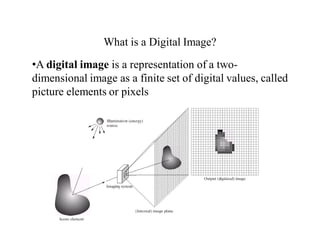
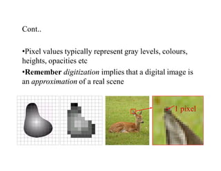
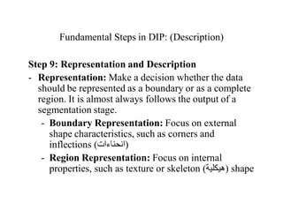
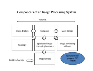
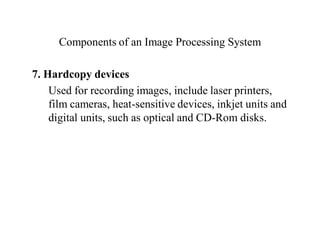
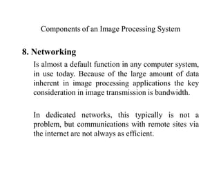
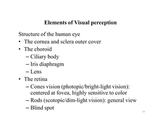
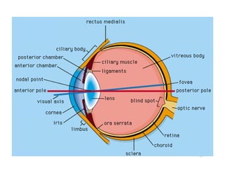
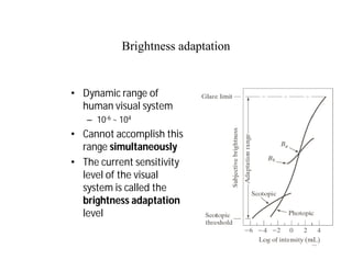
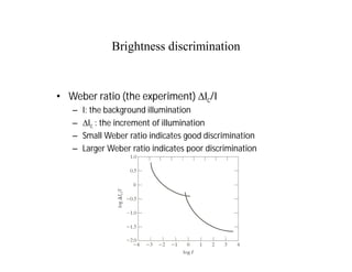
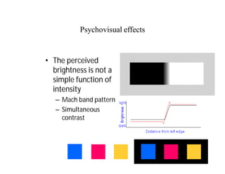
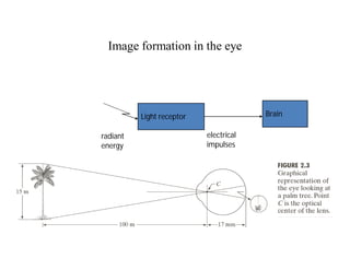
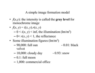
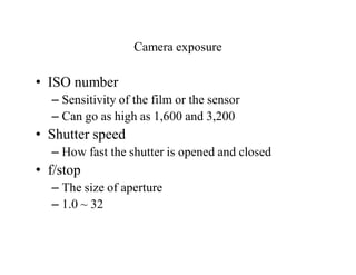
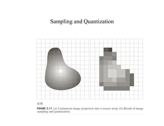
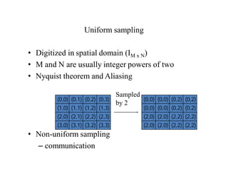
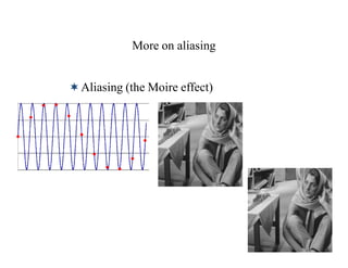
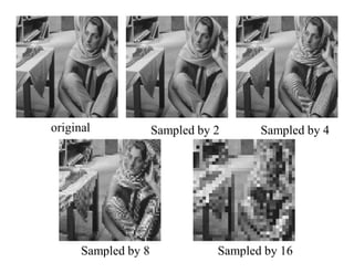
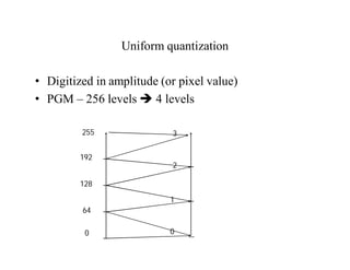
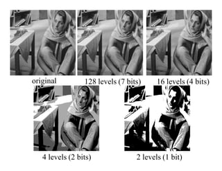
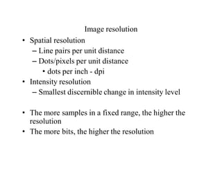
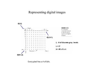
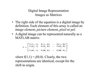
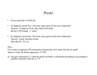
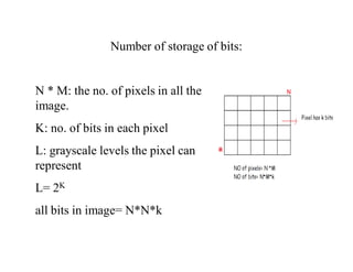
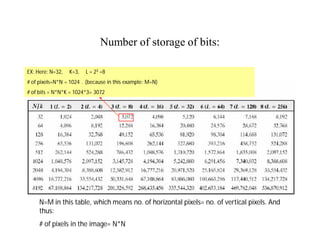
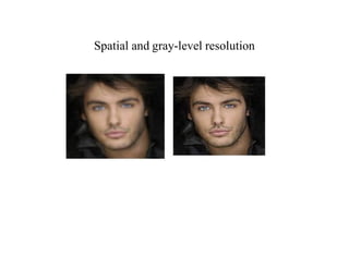
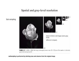
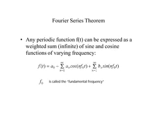
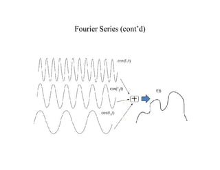
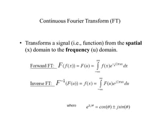
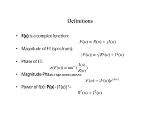
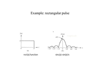
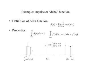
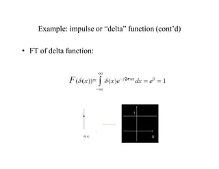
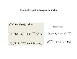
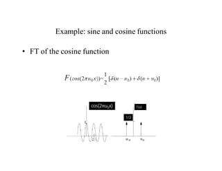
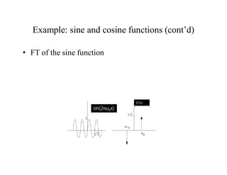
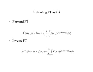
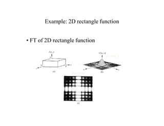
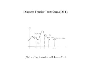
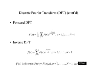
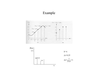
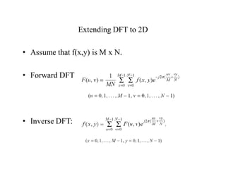
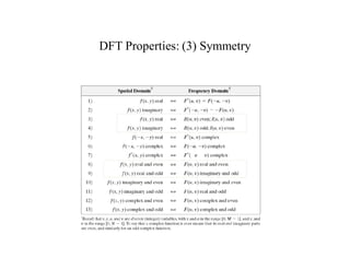
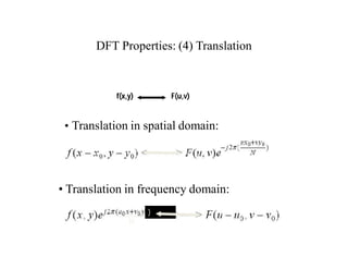
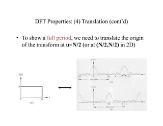
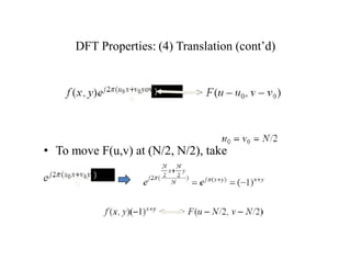
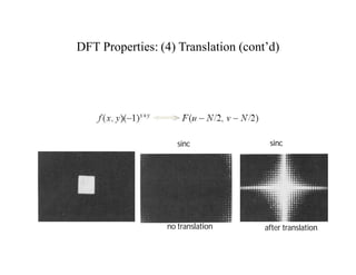
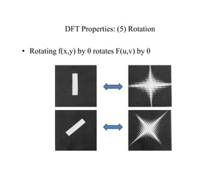
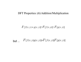
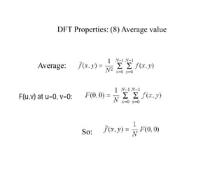
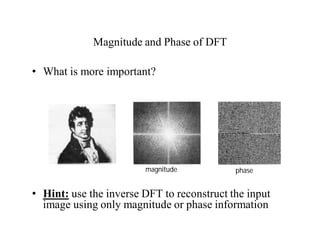
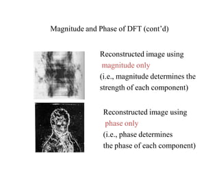
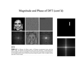
SlideShare a Scribd company logo
1 of 122
Download to read offline
BEC007-Digital Image Processing
UNIT I
DIGITAL IMAGE FUNDAMENTAL
• Elements of digital image processing systems
• Elements of Visual perception
• Image sampling and quantization
• Matrix and Singular Value representation of discrete
images.
What is a Digital Image?
•A digital image is a representation of a two-
dimensional image as a finite set of digital values, called
picture elements or pixels
Cont..
•Pixel values typically represent gray levels, colours,
heights, opacities etc
•Remember digitization implies that a digital image is
an approximation of a real scene
1 pixel
Cont..
Common image formats include:
1 sample per point (B&W or Grayscale)
3 samples per point (Red, Green, and Blue)
4 samples per point (Red, Green, Blue, and
“Alpha”, a.k.a. Opacity)
For most of this course we will focus on grey-
scale images
What is Digital Image Processing?
•Digital image processing focuses on two major tasks
– Improvement of pictorial information for human
interpretation
– Processing of image data for storage, transmission
and representation for autonomous machine
perception
•Some argument about where image processing ends
and fields such as image analysis and computer vision
start
cont…
The continuum from image processing to computer
vision can be broken up into low-, mid- and high-
level processes
History of Digital Image Processing
•Early 1920s: One of the first applications of digital
imaging was in the news-
paper industry
– The Bartlane cable picture
transmission service
– Images were transferred by submarine cable
between London and New York
– Pictures were coded for cable transfer and
reconstructed at the receiving end on a telegraph
printer
History of DIP (cont…)
•Mid to late 1920s: Improvements to the
Bartlane system resulted in higher quality images
– New reproduction
processes based
on photographic
techniques
– Increased number
of tones in
reproduced images
Improved
digital image Early 15 tone digital image
History of DIP (cont…)
•1960s: Improvements in computing technology
and the onset of the space race led to a surge of
work in digital image processing
– 1964: Computers used to
improve the quality of
images of the moon taken
by the Ranger 7 probe
– Such techniques were used
in other space missions
including the Apollo landings A picture of the moon taken by
the Ranger 7 probe minutes
before landing
History of DIP (cont…)
•1970s: Digital image processing begins to be
used in medical applications
– 1979: Sir Godfrey N.
Hounsfield & Prof. Allan M.
Cormack share the Nobel
Prize in medicine for the
invention of tomography,
the technology behind
Computerised Axial
Tomography (CAT) scans
Typical head slice CAT image
History of DIP (cont…)
•1980s - Today: The use of digital image processing
techniques has exploded and they are now used for all
kinds of tasks in all kinds of areas
– Image enhancement/restoration
– Artistic effects
– Medical visualisation
– Industrial inspection
– Law enforcement
– Human computer interfaces
Image Processing Fields
• Computer Graphics: The creation of images
• Image Processing: Enhancement or other
manipulation of the image
• Computer Vision: Analysis of the image content
Image Processing Fields
Input /
Output
Image Description
Image Image
Processing
Computer
Vision
Description Computer
Graphics
AI
Sometimes, Image Processing is defined as “a
discipline in which both the input and output of a
process are images
But, according to this classification, trivial tasks
of computing the average intensity of an image
would not be considered an image processing
operation
Computerized Processes Types
• Low-Level Processes:
– Input and output are images
– Tasks: Primitive operations, such as, image
processing to reduce noise, contrast enhancement
and image sharpening
Computerized Processes Types
• Mid-Level Processes:
– Inputs, generally, are images. Outputs are
attributes extracted from those images (edges,
contours, identity of individual objects)
– Tasks:
• Segmentation (partitioning an image into
regions or objects)
• Description of those objects to reduce them to a
form suitable for computer processing
• Classifications (recognition) of objects
Computerized Processes Types
• High-Level Processes:
– Image analysis and computer vision
Digital Image Definition
• An image can be defined as a two-dimensional
function f(x,y)
• x,y: Spatial coordinate
• F: the amplitude of any pair of coordinate x,y, which
is called the intensity or gray level of the image at
that point.
• X,y and f, are all finite and discrete quantities.
Fundamental Steps in Digital Image Processing:
Image
Acquisition
Image
Restoration
Morphological
Processing
Segmentation
Object
Recognition
Image
Enhancement Representation
& Description
Problem Domain
Colour Image
Processing
Image
Compression
Wavelets &
Multiresolution
processing
Knowledge Base
Outputs of these processes generally are images
Outputs
of
these
processes
generally
are
image
attributes
Fundamental Steps in DIP: (Description)
Step 1: Image Acquisition
The image is captured by a sensor (eg. Camera), and
digitized if the output of the camera or sensor is not
already in digital form, using analogue-to-digital
convertor
Fundamental Steps in DIP: (Description)
Step 2: Image Enhancement
The process of manipulating an image so that the
result is more suitable than the original for specific
applications.
The idea behind enhancement techniques is to bring
out details that are hidden, or simple to highlight
certain features of interest in an image.
Fundamental Steps in DIP: (Description)
Step 3: Image Restoration
- Improving the appearance of an image
- Tend to be mathematical or probabilistic models.
Enhancement, on the other hand, is based on human
subjective preferences regarding what constitutes a
“good” enhancement result.
Fundamental Steps in DIP: (Description)
Step 4: Colour Image Processing
Use the colour of the image to extract features of
interest in an image
Fundamental Steps in DIP: (Description)
Step 5: Wavelets
Are the foundation of representing images in various
degrees of resolution. It is used for image data
compression.
Fundamental Steps in DIP: (Description)
Step 6: Compression
Techniques for reducing the storage required to save
an image or the bandwidth required to transmit it.
Fundamental Steps in DIP: (Description)
Step 7: Morphological Processing
Tools for extracting image components that are useful
in the representation and description of shape.
In this step, there would be a transition from
processes that output images, to processes that output
image attributes.
Fundamental Steps in DIP: (Description)
Step 8: Image Segmentation
Segmentation procedures partition an image into its
constituent parts or objects.
Important Tip: The more accurate the
segmentation, the more likely recognition is to
succeed.
Fundamental Steps in DIP: (Description)
Step 9: Representation and Description
- Representation: Make a decision whether the data
should be represented as a boundary or as a complete
region. It is almost always follows the output of a
segmentation stage.
- Boundary Representation: Focus on external
shape characteristics, such as corners and
inflections (‫)اﻧﺤﻨﺎءات‬
- Region Representation: Focus on internal
properties, such as texture or skeleton (‫)ھﯿﻜﻠﯿﺔ‬ shape
Fundamental Steps in DIP: (Description)
Step 9: Representation and Description
- Choosing a representation is only part of the solution
for transforming raw data into a form suitable for
subsequent computer processing (mainly recognition)
- Description: also called, feature selection, deals with
extracting attributes that result in some information of
interest.
Fundamental Steps in DIP: (Description)
Step 9: Recognition and Interpretation
Recognition: the process that assigns label to an
object based on the information provided by its
description.
Fundamental Steps in DIP: (Description)
Step 10: Knowledge Base
Knowledge about a problem domain is coded into an
image processing system in the form of a knowledge
database.
Components of an Image Processing System
Network
Image displays Computer Mass storage
Hardcopy
Specialized image
processing hardware
Image processing
software
Image sensors
Problem Domain
Typical general-
purpose DIP
system
Components of an Image Processing System
1. Image Sensors
Two elements are required to acquire digital images.
The first is the physical device that is sensitive to the
energy radiated by the object we wish to image
(Sensor). The second, called a digitizer, is a device
for converting the output of the physical sensing
device into digital form.
Components of an Image Processing System
2. Specialized Image Processing Hardware
Usually consists of the digitizer, mentioned before,
plus hardware that performs other primitive
operations, such as an arithmetic logic unit (ALU),
which performs arithmetic and logical operations in
parallel on entire images.
This type of hardware sometimes is called a front-
end subsystem, and its most distinguishing
characteristic is speed. In other words, this unit
performs functions that require fast data throughputs
that the typical main computer cannot handle.
Components of an Image Processing System
3. Computer
The computer in an image processing system is a
general-purpose computer and can range from a PC
to a supercomputer. In dedicated applications,
sometimes specially designed computers are used to
achieve a required level of performance.
Components of an Image Processing System
4. Image Processing Software
Software for image processing consists of
specialized modules that perform specific tasks. A
well-designed package also includes the capability
for the user to write code that, as a minimum,
utilizes the specialized modules.
Components of an Image Processing System
5. Mass Storage Capability
Mass storage capability is a must in a image
processing applications. And image of sized 1024 *
1024 pixels requires one megabyte of storage space
if the image is not compressed.
Digital storage for image processing applications
falls into three principal categories:
1. Short-term storage for use during processing.
2. on line storage for relatively fast recall
3. Archival storage, characterized by infrequent
access
Components of an Image Processing System
5. Mass Storage Capability
One method of providing short-term storage is
computer memory. Another is by specialized boards,
called frame buffers, that store one or more images
and can be accessed rapidly.
The on-line storage method, allows virtually
instantaneous image zoom, as well as scroll (vertical
shifts) and pan (horizontal shifts). On-line storage
generally takes the form of magnetic disks and
optical-media storage. The key factor characterizing
on-line storage is frequent access to the stored data.
Components of an Image Processing System
6. Image Displays
The displays in use today are mainly color
(preferably flat screen) TV monitors. Monitors are
driven by the outputs of the image and graphics
display cards that are an integral part of a computer
system.
Components of an Image Processing System
7. Hardcopy devices
Used for recording images, include laser printers,
film cameras, heat-sensitive devices, inkjet units and
digital units, such as optical and CD-Rom disks.
Components of an Image Processing System
8. Networking
Is almost a default function in any computer system,
in use today. Because of the large amount of data
inherent in image processing applications the key
consideration in image transmission is bandwidth.
In dedicated networks, this typically is not a
problem, but communications with remote sites via
the internet are not always as efficient.
44
Elements of Visual perception
Structure of the human eye
• The cornea and sclera outer cover
• The choroid
– Ciliary body
– Iris diaphragm
– Lens
• The retina
– Cones vision (photopic/bright-light vision):
centered at fovea, highly sensitive to color
– Rods (scotopic/dim-light vision): general view
– Blind spot
45
Human eye
Cones vs. Rods
Hexagonal pixel
•Models human visual system more precisely
•The distance between a given pixel and its
immediate neighbors is the same
•Hexagonal sampling requires 13% fewer
samples than rectangular sampling
•ANN can be trained with less errors
Cone distribution on the
fovea (200,000 cones/mm2)
More on the cone
mosaic
The cone mosaic of fish retina
Lythgoe, Ecology of Vision (1979)
Human retina mosaic
-Irregularity reduces visual
acuity for high-frequency signals
-Introduce random noise
The mosaic array of most
vertebrates is regular
A mosaicked multispectral camera
50
Brightness adaptation
• Dynamic range of
human visual system
– 10-6 ~ 104
• Cannot accomplish this
range simultaneously
• The current sensitivity
level of the visual
system is called the
brightness adaptation
level
Brightness discrimination
• Weber ratio (the experiment) DIc/I
– I: the background illumination
– DIc : the increment of illumination
– Small Weber ratio indicates good discrimination
– Larger Weber ratio indicates poor discrimination
52
Psychovisual effects
• The perceived
brightness is not a
simple function of
intensity
– Mach band pattern
– Simultaneous
contrast
Image formation in the eye
• Flexible lens
• Controlled by the tension in the fibers of the
ciliary body
– To focus on distant objects?
– To focus on objects near eye?
– Near-sighted and far-sighted
Image formation in the eye
Light receptor
radiant
energy
electrical
impulses
Brain
A simple image formation model
• f(x,y): the intensity is called the gray level for
monochrome image
• f(x, y) = i(x, y).r(x, y)
– 0 < i(x, y) < inf, the illumination (lm/m2)
– 0< r(x, y) < 1, the reflectance
• Some illumination figures (lm/m2)
– 90,000: full sun - 0.01: black
velvet
– 10,000: cloudy day - 0.93: snow
– 0.1: full moon
– 1,000: commercial office
Camera exposure
• ISO number
– Sensitivity of the film or the sensor
– Can go as high as 1,600 and 3,200
• Shutter speed
– How fast the shutter is opened and closed
• f/stop
– The size of aperture
– 1.0 ~ 32
Sampling and Quantization
Uniform sampling
• Digitized in spatial domain (IM x N)
• M and N are usually integer powers of two
• Nyquist theorem and Aliasing
• Non-uniform sampling
– communication
(0,0) (0,1) (0,2) (0,3)
(1,0)
(3,0)
(2,0)
(1,1)
(2,1)
(3,1)
(2,2)
(3,2)
(1,2)
(3,3)
(2,3)
(1,3)
(0,0) (0,0) (0,2) (0,2)
(0,0)
(2,0)
(2,0)
(0,0)
(2,0)
(2,0)
(2,2)
(2,2)
(0,2)
(2,2)
(2,2)
(0,2)
Sampled
by 2
59
More on aliasing
Aliasing (the Moire effect)
original Sampled by 2 Sampled by 4
Sampled by 8 Sampled by 16
Uniform quantization
• Digitized in amplitude (or pixel value)
• PGM – 256 levels  4 levels
0
255
64
128
192
0
3
1
2
original 128 levels (7 bits) 16 levels (4 bits)
4 levels (2 bits) 2 levels (1 bit)
Image resolution
• Spatial resolution
– Line pairs per unit distance
– Dots/pixels per unit distance
• dots per inch - dpi
• Intensity resolution
– Smallest discernible change in intensity level
• The more samples in a fixed range, the higher the
resolution
• The more bits, the higher the resolution
3D interpretation of line drawing
• Emulation approach
– A given 3-D interpretation is considered less likely
to be correct if some angles between the wires are
much larger than others
Representing digital images
Every pixel has a # of bits.
Digital Image Representation Coordinate Conventions
• The result of sampling and quantization is a matrix of real
numbers
• There are two principle ways to represent a digital image:
– Assume that an image f(x,y) is sampled so that the resulting
image has M rows and N columns. We say that the image is
of size
M x N. The values of the coordinates (x,y) are discrete
quantities. For clarity, we use integer values for these
discrete coordinates.
In many image processing books, the image origin is
defined to be at (x,y) = (0,0). The next coordinate values
along the first row of the image are (x,y) = (0,1). It is
important to keep in mind that the notation (0,1) is used to
signify the second sample along the first row. It does not
mean that these are the actual values of physical
coordinates. Note that x ranges from 0 to M-1, and y ranges
from 0 to N-1. Figure (a)
Digital Image Representation Coordinate Conventions
– The coordinate convention used in toolbox to
denote arrays is different from the preceding
paragraph in two minor ways.
• Instead of using (x,y) the toolbox uses the
notation (r,c) to indicate rows and columns.
• The origin of the coordinate system is at (r,c) =
(1,1); thus, r ranges from 1 to M and c from 1 to
N, in integer increments. This coordinate
convention is shown in Figure (b).
Digital Image Representation Coordinate Conventions
(A) (B)
Digital Image Representation
Images as Matrices
• The coordination system in figure (A) and the
preceding discussion lead to the following
representation for a digitized image function:
Digital Image Representation
Images as Matrices
• The right side of the equation is a digital image by
definition. Each element of this array is called an
image element, picture element, pixel or pel.
• A digital image can be represented naturally as a
MATLAB matrix:
Where f(1,1) = f(0,0). Clearly, the two
representations are identical, except for the
shift in origin.
Pixels!
• Every pixel has # of bits (k)
• Q: Suppose a pixel has 1 bit, how many gray levels can it represent?
Answer: 2 intensity levels only, black and white.
Bit (0,1)  0:black , 1: white
• Q: Suppose a pixel has 2 bit, how many gray levels can it represent?
Answer: 4 gray intensity levels
2Bit (00, 01, 10 ,11).
Now ..
if we want to represent 256 intensities of grayscale, how many bits do we need?
Answer: 8 bits  which represents: 28=256
so, the gray intensities ( L ) that the pixel can hold, is calculated according to according to
number of pixels it has (k). L= 2k
Number of storage of bits:
N * M: the no. of pixels in all the
image.
K: no. of bits in each pixel
L: grayscale levels the pixel can
represent
L= 2K
all bits in image= N*N*k
Number of storage of bits:
EX: Here: N=32, K=3, L = 23 =8
# of pixels=N*N = 1024 . (because in this example: M=N)
# of bits = N*N*K = 1024*3= 3072
N=M in this table, which means no. of horizontal pixels= no. of vertical pixels. And
thus:
# of pixels in the image= N*N
Spatial and gray-level resolution
• Sampling is the principal factor determining the spatial
resolution of an image
• Basically, spatial resolution is the smallest discernible
detail in an image.
• Spatial Resolution
Spatial and gray-level resolution
• Gray-level resolution refers to the smallest discernible
change in gray level.
Spatial and gray-level resolution
subSampling is performed by deleting rows and columns from the original image.
Same # of bits in all images (same gray
level)
different # of pixels
Sub sampling
Spatial and gray-level resolution
Resampling is performed by row and column duplication
Re sampling
(pixel replication)
A special case of nearest
neighbor zooming.
UNIT II
IMAGE TRANSFORMS
• 1D DFT
• 2D DFT
• Cosine
• Sine Hadamard
• Hear
• Slant
• KL
• SVD transform and their properties.
Image Transforms
• Many times, image processing tasks are best
performed in a domain other than the
spatial domain.
• Key steps
(1) Transform the image
(2) Carry the task(s) in the transformed domain.
(3) Apply inverse transform to return to the
spatial domain.
Transformation Kernels
• Forward Transformation
• Inverse Transformation










1
0
1
0
1
,...,
1
,
0
,
1
,...,
1
,
0
)
,
,
,
(
)
,
(
)
,
(
M
x
N
y
N
v
M
u
v
u
y
x
r
y
x
f
v
u
T










1
0
1
0
1
,...,
1
,
0
,
1
,...,
1
,
0
)
,
,
,
(
)
,
(
)
,
(
M
u
N
v
N
y
M
x
v
u
y
x
s
v
u
T
y
x
f
inverse transformation kernel
forward transformation kernel
Kernel Properties
• A kernel is said to be separable if:
• A kernel is said to be symmetric if:
)
,
(
)
,
(
)
,
,
,
( 2
1 v
y
r
u
x
r
v
u
y
x
r 
)
,
(
)
,
(
)
,
,
,
( 1
1 v
y
r
u
x
r
v
u
y
x
r 
Fourier Series Theorem
• Any periodic function f(t) can be expressed as a
weighted sum (infinite) of sine and cosine
functions of varying frequency:
is called the “fundamental frequency”
Fourier Series (cont’d)
α1
α2
α3
Continuous Fourier Transform (FT)
• Transforms a signal (i.e., function) from the spatial
(x) domain to the frequency (u) domain.
where
Definitions
• F(u) is a complex function:
• Magnitude of FT (spectrum):
• Phase of FT:
• Magnitude-Phase representation:
• Power of f(x): P(u)=|F(u)|2=
Why is FT Useful?
• Easier to remove undesirable frequencies in the
frequency domain.
• Faster to perform certain operations in the frequency
domain than in the spatial domain.
Example: Removing undesirable frequencies
remove high
frequencies
reconstructed
signal
frequencies
noisy signal
To remove certain
frequencies, set their
corresponding F(u)
coefficients to zero!
How do frequencies show up in an image?
• Low frequencies correspond to slowly varying pixel
intensities (e.g., continuous surface).
• High frequencies correspond to quickly varying pixel
intensities (e.g., edges)
Original Image Low-passed
Example of noise reduction using FT
Input image
Output image
Spectrum (frequency domain)
Band-reject
filter
Frequency Filtering: Main Steps
1. Take the FT of f(x):
2. Remove undesired frequencies:
3. Convert back to a signal:
Example: rectangular pulse
rect(x) function sinc(x)=sin(x)/x
magnitude
Example: impulse or “delta” function
• Definition of delta function:
• Properties:
Example: impulse or “delta” function (cont’d)
• FT of delta function:
1
u
x
Example: spatial/frequency shifts
)
(
)
(
)
2
(
)
(
)
(
)
1
(
),
(
)
(
0
2
2
0
0
0
u
u
F
e
x
f
u
F
e
x
x
f
then
u
F
x
f
x
u
j
ux
j








Special Cases:
0
2
0 )
( ux
j
e
x
x 
 


)
( 0
2 0
u
u
e x
u
j

 

Example: sine and cosine functions
• FT of the cosine function
cos(2πu0x)
1/2
F(u)
Example: sine and cosine functions (cont’d)
• FT of the sine function
sin(2πu0x)
jF(u)
Extending FT in 2D
• Forward FT
• Inverse FT
Example: 2D rectangle function
• FT of 2D rectangle function
2D sinc()
top view
Discrete Fourier Transform (DFT)
Discrete Fourier Transform (DFT) (cont’d)
• Forward DFT
• Inverse DFT
1/(NΔx)
Example
Extending DFT to 2D
• Assume that f(x,y) is M x N.
• Forward DFT
• Inverse DFT:
Extending DFT to 2D (cont’d)
• Special case: f(x,y) is N x N.
• Forward DFT
• Inverse DFT
u,v = 0,1,2, …, N-1
x,y = 0,1,2, …, N-1
Extending DFT to 2D (cont’d)
2D cos/sin functions
Interpretation:
Visualizing DFT
• Typically, we visualize |F(u,v)|
• The dynamic range of |F(u,v)| is typically very large
• Apply streching: (c is const)
before stretching after stretching
original image
|F(u,v)| |D(u,v)|
DFT Properties: (1) Separability
• The 2D DFT can be computed using 1D transforms
only:
Forward DFT:
2 ( ) 2 ( ) 2 ( )
ux vy ux vy
j j j
N N N
e e e
  

  

kernel is
separable:
DFT Properties: (1) Separability (cont’d)
• Rewrite F(u,v) as follows:
• Let’s set:
• Then:
DFT Properties: (1) Separability (cont’d)
• How can we compute F(x,v)?
• How can we compute F(u,v)?
)
N x DFT of rows of f(x,y)
DFT of cols of F(x,v)
DFT Properties: (1) Separability (cont’d)
DFT Properties: (2) Periodicity
• The DFT and its inverse are periodic with period N
DFT Properties: (3) Symmetry
DFT Properties: (4) Translation
f(x,y) F(u,v)
)
N
• Translation in spatial domain:
• Translation in frequency domain:
DFT Properties: (4) Translation (cont’d)
• To show a full period, we need to translate the origin
of the transform at u=N/2 (or at (N/2,N/2) in 2D)
|F(u-N/2)|
|F(u)|
DFT Properties: (4) Translation (cont’d)
• To move F(u,v) at (N/2, N/2), take
)
N
)
N
DFT Properties: (4) Translation (cont’d)
no translation after translation
sinc
sinc
DFT Properties: (5) Rotation
• Rotating f(x,y) by θ rotates F(u,v) by θ
DFT Properties: (6) Addition/Multiplication
but …
DFT Properties: (8) Average value
So:
Average:
F(u,v) at u=0, v=0:
Magnitude and Phase of DFT
• What is more important?
• Hint: use the inverse DFT to reconstruct the input
image using only magnitude or phase information
magnitude phase
Magnitude and Phase of DFT (cont’d)
Reconstructed image using
magnitude only
(i.e., magnitude determines the
strength of each component)
Reconstructed image using
phase only
(i.e., phase determines
the phase of each component)
Magnitude and Phase of DFT (cont’d)
only phase
only magnitude phase (woman)
magnitude (rectangle)
phase (rectangle)
magnitude (woman)

More Related Content

What's hot

Frequency Domain FIltering.pdf
Frequency Domain FIltering.pdfFrequency Domain FIltering.pdf
Frequency Domain FIltering.pdfMuhammad_Ilham_21
 
Wavelet based image compression technique
Wavelet based image compression techniqueWavelet based image compression technique
Wavelet based image compression techniquePriyanka Pachori
 
Color image processing Presentation
Color image processing PresentationColor image processing Presentation
Color image processing PresentationRevanth Chimmani
 
Image Enhancement using Frequency Domain Filters
Image Enhancement using Frequency Domain FiltersImage Enhancement using Frequency Domain Filters
Image Enhancement using Frequency Domain FiltersKarthika Ramachandran
 
Licence plate recognition using matlab programming
Licence plate recognition using matlab programming Licence plate recognition using matlab programming
Licence plate recognition using matlab programming somchaturvedi
 
DIP Notes Unit-1 PPT.pdf
DIP Notes Unit-1 PPT.pdfDIP Notes Unit-1 PPT.pdf
DIP Notes Unit-1 PPT.pdfGaurav Sharma
 
Edge Detection and Segmentation
Edge Detection and SegmentationEdge Detection and Segmentation
Edge Detection and SegmentationA B Shinde
 
Lec 07 image enhancement in frequency domain i
Lec 07 image enhancement in frequency domain iLec 07 image enhancement in frequency domain i
Lec 07 image enhancement in frequency domain iAli Hassan
 
Lect 02 first portion
Lect 02   first portionLect 02   first portion
Lect 02 first portionMoe Moe Myint
 
Image segmentation in Digital Image Processing
Image segmentation in Digital Image ProcessingImage segmentation in Digital Image Processing
Image segmentation in Digital Image ProcessingDHIVYADEVAKI
 
Image Acquisition and Representation
Image Acquisition and RepresentationImage Acquisition and Representation
Image Acquisition and RepresentationAmnaakhaan
 
Digitized images and
Digitized images andDigitized images and
Digitized images andAshish Kumar
 
Introduction to Digital Image Processing
Introduction to Digital Image ProcessingIntroduction to Digital Image Processing
Introduction to Digital Image Processingkalaimuthu2
 
Digital Image restoration
Digital Image restorationDigital Image restoration
Digital Image restorationMd Shabir Alam
 
Wavelet transform in two dimensions
Wavelet transform in two dimensionsWavelet transform in two dimensions
Wavelet transform in two dimensionsAyushi Gagneja
 
Predictive coding
Predictive codingPredictive coding
Predictive codingp_ayal
 
Digital Image Fundamentals
Digital Image FundamentalsDigital Image Fundamentals
Digital Image FundamentalsA B Shinde
 

What's hot (20)

Frequency Domain FIltering.pdf
Frequency Domain FIltering.pdfFrequency Domain FIltering.pdf
Frequency Domain FIltering.pdf
 
Wavelet based image compression technique
Wavelet based image compression techniqueWavelet based image compression technique
Wavelet based image compression technique
 
Color image processing Presentation
Color image processing PresentationColor image processing Presentation
Color image processing Presentation
 
Image Enhancement using Frequency Domain Filters
Image Enhancement using Frequency Domain FiltersImage Enhancement using Frequency Domain Filters
Image Enhancement using Frequency Domain Filters
 
Image enhancement
Image enhancementImage enhancement
Image enhancement
 
Licence plate recognition using matlab programming
Licence plate recognition using matlab programming Licence plate recognition using matlab programming
Licence plate recognition using matlab programming
 
DIP Notes Unit-1 PPT.pdf
DIP Notes Unit-1 PPT.pdfDIP Notes Unit-1 PPT.pdf
DIP Notes Unit-1 PPT.pdf
 
Edge Detection and Segmentation
Edge Detection and SegmentationEdge Detection and Segmentation
Edge Detection and Segmentation
 
Lec 07 image enhancement in frequency domain i
Lec 07 image enhancement in frequency domain iLec 07 image enhancement in frequency domain i
Lec 07 image enhancement in frequency domain i
 
Lect 02 first portion
Lect 02   first portionLect 02   first portion
Lect 02 first portion
 
Image segmentation in Digital Image Processing
Image segmentation in Digital Image ProcessingImage segmentation in Digital Image Processing
Image segmentation in Digital Image Processing
 
Image Acquisition and Representation
Image Acquisition and RepresentationImage Acquisition and Representation
Image Acquisition and Representation
 
Digitized images and
Digitized images andDigitized images and
Digitized images and
 
Introduction to Digital Image Processing
Introduction to Digital Image ProcessingIntroduction to Digital Image Processing
Introduction to Digital Image Processing
 
Image segmentation
Image segmentationImage segmentation
Image segmentation
 
Digital Image restoration
Digital Image restorationDigital Image restoration
Digital Image restoration
 
Wavelet transform in two dimensions
Wavelet transform in two dimensionsWavelet transform in two dimensions
Wavelet transform in two dimensions
 
Predictive coding
Predictive codingPredictive coding
Predictive coding
 
Digital Image Fundamentals
Digital Image FundamentalsDigital Image Fundamentals
Digital Image Fundamentals
 
Image Sensing and Aquisition
Image Sensing and AquisitionImage Sensing and Aquisition
Image Sensing and Aquisition
 

Similar to BEC007 -Digital image processing.pdf

Digital_image_processing_-Vijaya_Raghavan.pdf
Digital_image_processing_-Vijaya_Raghavan.pdfDigital_image_processing_-Vijaya_Raghavan.pdf
Digital_image_processing_-Vijaya_Raghavan.pdfVaideshSiva1
 
Basics of digital image processing
Basics of digital image  processingBasics of digital image  processing
Basics of digital image processingzahid6
 
Digital Image Processing
Digital Image ProcessingDigital Image Processing
Digital Image ProcessingReshma KC
 
Computer Graphics Unit 5 notes for Manonmanium Sundaranar University
Computer Graphics  Unit 5 notes for Manonmanium Sundaranar UniversityComputer Graphics  Unit 5 notes for Manonmanium Sundaranar University
Computer Graphics Unit 5 notes for Manonmanium Sundaranar UniversityRajeswariR45
 
Fundamentals of Image Processing & Components.ppt
Fundamentals of Image Processing & Components.pptFundamentals of Image Processing & Components.ppt
Fundamentals of Image Processing & Components.pptANJANISINGHAL
 
Chap_1_Digital_Image_Fundamentals_DD (2).pdf
Chap_1_Digital_Image_Fundamentals_DD (2).pdfChap_1_Digital_Image_Fundamentals_DD (2).pdf
Chap_1_Digital_Image_Fundamentals_DD (2).pdfMrNeon5
 
Image Processing Basics
Image Processing BasicsImage Processing Basics
Image Processing BasicsA B Shinde
 
DIPsadasdasfsdfsdfdfasdfsdfsdgsdgdsfgdfgfdg
DIPsadasdasfsdfsdfdfasdfsdfsdgsdgdsfgdfgfdgDIPsadasdasfsdfsdfdfasdfsdfsdgsdgdsfgdfgfdg
DIPsadasdasfsdfsdfdfasdfsdfsdgsdgdsfgdfgfdgMrVMNair
 
Unit 1 DIP Fundamentals - Presentation Notes.pdf
Unit 1 DIP Fundamentals - Presentation Notes.pdfUnit 1 DIP Fundamentals - Presentation Notes.pdf
Unit 1 DIP Fundamentals - Presentation Notes.pdfsdbhosale860
 
Fundamental Steps Of Image Processing
Fundamental Steps Of Image ProcessingFundamental Steps Of Image Processing
Fundamental Steps Of Image ProcessingSouma Maiti
 
Fundamental steps in image processing
Fundamental steps in image processingFundamental steps in image processing
Fundamental steps in image processingPremaPRC211300301103
 

Similar to BEC007 -Digital image processing.pdf (20)

imp.pptx
imp.pptximp.pptx
imp.pptx
 
Digital_image_processing_-Vijaya_Raghavan.pdf
Digital_image_processing_-Vijaya_Raghavan.pdfDigital_image_processing_-Vijaya_Raghavan.pdf
Digital_image_processing_-Vijaya_Raghavan.pdf
 
Basics of digital image processing
Basics of digital image  processingBasics of digital image  processing
Basics of digital image processing
 
mca.pptx
mca.pptxmca.pptx
mca.pptx
 
Digital Image Processing
Digital Image ProcessingDigital Image Processing
Digital Image Processing
 
Computer Graphics Unit 5 notes for Manonmanium Sundaranar University
Computer Graphics  Unit 5 notes for Manonmanium Sundaranar UniversityComputer Graphics  Unit 5 notes for Manonmanium Sundaranar University
Computer Graphics Unit 5 notes for Manonmanium Sundaranar University
 
Fundamentals of Image Processing & Components.ppt
Fundamentals of Image Processing & Components.pptFundamentals of Image Processing & Components.ppt
Fundamentals of Image Processing & Components.ppt
 
Dip review
Dip reviewDip review
Dip review
 
Chap_1_Digital_Image_Fundamentals_DD (2).pdf
Chap_1_Digital_Image_Fundamentals_DD (2).pdfChap_1_Digital_Image_Fundamentals_DD (2).pdf
Chap_1_Digital_Image_Fundamentals_DD (2).pdf
 
Image Processing Basics
Image Processing BasicsImage Processing Basics
Image Processing Basics
 
DIPsadasdasfsdfsdfdfasdfsdfsdgsdgdsfgdfgfdg
DIPsadasdasfsdfsdfdfasdfsdfsdgsdgdsfgdfgfdgDIPsadasdasfsdfsdfdfasdfsdfsdgsdgdsfgdfgfdg
DIPsadasdasfsdfsdfdfasdfsdfsdgsdgdsfgdfgfdg
 
DIP
DIPDIP
DIP
 
Ch1.pptx
Ch1.pptxCh1.pptx
Ch1.pptx
 
Unit 1 DIP Fundamentals - Presentation Notes.pdf
Unit 1 DIP Fundamentals - Presentation Notes.pdfUnit 1 DIP Fundamentals - Presentation Notes.pdf
Unit 1 DIP Fundamentals - Presentation Notes.pdf
 
1 dip introduction
1 dip introduction1 dip introduction
1 dip introduction
 
Dip
DipDip
Dip
 
Fundamental Steps Of Image Processing
Fundamental Steps Of Image ProcessingFundamental Steps Of Image Processing
Fundamental Steps Of Image Processing
 
Digital image processing
Digital image processingDigital image processing
Digital image processing
 
ACMP340.pptx
ACMP340.pptxACMP340.pptx
ACMP340.pptx
 
Fundamental steps in image processing
Fundamental steps in image processingFundamental steps in image processing
Fundamental steps in image processing
 

More from gopikahari7

Tema2_ArchitectureMIPS.pptx
Tema2_ArchitectureMIPS.pptxTema2_ArchitectureMIPS.pptx
Tema2_ArchitectureMIPS.pptxgopikahari7
 
cuckoosearchalgorithm-141028173457-conversion-gate02 (1).pptx
cuckoosearchalgorithm-141028173457-conversion-gate02 (1).pptxcuckoosearchalgorithm-141028173457-conversion-gate02 (1).pptx
cuckoosearchalgorithm-141028173457-conversion-gate02 (1).pptxgopikahari7
 
Final PPT.pptx (1).pptx
Final PPT.pptx (1).pptxFinal PPT.pptx (1).pptx
Final PPT.pptx (1).pptxgopikahari7
 
S12075-GPU-Accelerated-Video-Encoding.pptx
S12075-GPU-Accelerated-Video-Encoding.pptxS12075-GPU-Accelerated-Video-Encoding.pptx
S12075-GPU-Accelerated-Video-Encoding.pptxgopikahari7
 
S12075-GPU-Accelerated-Video-Encoding.pdf
S12075-GPU-Accelerated-Video-Encoding.pdfS12075-GPU-Accelerated-Video-Encoding.pdf
S12075-GPU-Accelerated-Video-Encoding.pdfgopikahari7
 
batalgorithm-160501121237 (1).pptx
batalgorithm-160501121237 (1).pptxbatalgorithm-160501121237 (1).pptx
batalgorithm-160501121237 (1).pptxgopikahari7
 
batalgorithm-170406072944 (4).pptx
batalgorithm-170406072944 (4).pptxbatalgorithm-170406072944 (4).pptx
batalgorithm-170406072944 (4).pptxgopikahari7
 
Copy of Parallel_and_Cluster_Computing.pptx
Copy of Parallel_and_Cluster_Computing.pptxCopy of Parallel_and_Cluster_Computing.pptx
Copy of Parallel_and_Cluster_Computing.pptxgopikahari7
 
MattsonTutorialSC14.pptx
MattsonTutorialSC14.pptxMattsonTutorialSC14.pptx
MattsonTutorialSC14.pptxgopikahari7
 
batalgorithm-170406072944 (4).pptx
batalgorithm-170406072944 (4).pptxbatalgorithm-170406072944 (4).pptx
batalgorithm-170406072944 (4).pptxgopikahari7
 
ELEMPowerPoint.pptx
ELEMPowerPoint.pptxELEMPowerPoint.pptx
ELEMPowerPoint.pptxgopikahari7
 
plantpresentation.ppt
plantpresentation.pptplantpresentation.ppt
plantpresentation.pptgopikahari7
 
2_2018_12_20!06_04_28_PM.ppt
2_2018_12_20!06_04_28_PM.ppt2_2018_12_20!06_04_28_PM.ppt
2_2018_12_20!06_04_28_PM.pptgopikahari7
 
abelbrownnvidiarakuten2016-170208065814 (1).pptx
abelbrownnvidiarakuten2016-170208065814 (1).pptxabelbrownnvidiarakuten2016-170208065814 (1).pptx
abelbrownnvidiarakuten2016-170208065814 (1).pptxgopikahari7
 
realtime_ai_systems_academia.pptx
realtime_ai_systems_academia.pptxrealtime_ai_systems_academia.pptx
realtime_ai_systems_academia.pptxgopikahari7
 
ppd_seminar_110202_talk_edward_freeman_introduction_to_programmable_logic_dev...
ppd_seminar_110202_talk_edward_freeman_introduction_to_programmable_logic_dev...ppd_seminar_110202_talk_edward_freeman_introduction_to_programmable_logic_dev...
ppd_seminar_110202_talk_edward_freeman_introduction_to_programmable_logic_dev...gopikahari7
 

More from gopikahari7 (20)

Tema2_ArchitectureMIPS.pptx
Tema2_ArchitectureMIPS.pptxTema2_ArchitectureMIPS.pptx
Tema2_ArchitectureMIPS.pptx
 
barrera.ppt
barrera.pptbarrera.ppt
barrera.ppt
 
cuckoosearchalgorithm-141028173457-conversion-gate02 (1).pptx
cuckoosearchalgorithm-141028173457-conversion-gate02 (1).pptxcuckoosearchalgorithm-141028173457-conversion-gate02 (1).pptx
cuckoosearchalgorithm-141028173457-conversion-gate02 (1).pptx
 
Final PPT.pptx (1).pptx
Final PPT.pptx (1).pptxFinal PPT.pptx (1).pptx
Final PPT.pptx (1).pptx
 
S12075-GPU-Accelerated-Video-Encoding.pptx
S12075-GPU-Accelerated-Video-Encoding.pptxS12075-GPU-Accelerated-Video-Encoding.pptx
S12075-GPU-Accelerated-Video-Encoding.pptx
 
S12075-GPU-Accelerated-Video-Encoding.pdf
S12075-GPU-Accelerated-Video-Encoding.pdfS12075-GPU-Accelerated-Video-Encoding.pdf
S12075-GPU-Accelerated-Video-Encoding.pdf
 
batalgorithm-160501121237 (1).pptx
batalgorithm-160501121237 (1).pptxbatalgorithm-160501121237 (1).pptx
batalgorithm-160501121237 (1).pptx
 
batalgorithm-170406072944 (4).pptx
batalgorithm-170406072944 (4).pptxbatalgorithm-170406072944 (4).pptx
batalgorithm-170406072944 (4).pptx
 
Copy of Parallel_and_Cluster_Computing.pptx
Copy of Parallel_and_Cluster_Computing.pptxCopy of Parallel_and_Cluster_Computing.pptx
Copy of Parallel_and_Cluster_Computing.pptx
 
MattsonTutorialSC14.pptx
MattsonTutorialSC14.pptxMattsonTutorialSC14.pptx
MattsonTutorialSC14.pptx
 
batalgorithm-170406072944 (4).pptx
batalgorithm-170406072944 (4).pptxbatalgorithm-170406072944 (4).pptx
batalgorithm-170406072944 (4).pptx
 
ELEMPowerPoint.pptx
ELEMPowerPoint.pptxELEMPowerPoint.pptx
ELEMPowerPoint.pptx
 
Hayes2010.ppt
Hayes2010.pptHayes2010.ppt
Hayes2010.ppt
 
plantpresentation.ppt
plantpresentation.pptplantpresentation.ppt
plantpresentation.ppt
 
Plants.ppt
Plants.pptPlants.ppt
Plants.ppt
 
2_2018_12_20!06_04_28_PM.ppt
2_2018_12_20!06_04_28_PM.ppt2_2018_12_20!06_04_28_PM.ppt
2_2018_12_20!06_04_28_PM.ppt
 
abelbrownnvidiarakuten2016-170208065814 (1).pptx
abelbrownnvidiarakuten2016-170208065814 (1).pptxabelbrownnvidiarakuten2016-170208065814 (1).pptx
abelbrownnvidiarakuten2016-170208065814 (1).pptx
 
realtime_ai_systems_academia.pptx
realtime_ai_systems_academia.pptxrealtime_ai_systems_academia.pptx
realtime_ai_systems_academia.pptx
 
ppd_seminar_110202_talk_edward_freeman_introduction_to_programmable_logic_dev...
ppd_seminar_110202_talk_edward_freeman_introduction_to_programmable_logic_dev...ppd_seminar_110202_talk_edward_freeman_introduction_to_programmable_logic_dev...
ppd_seminar_110202_talk_edward_freeman_introduction_to_programmable_logic_dev...
 
FPGA-Arch.ppt
FPGA-Arch.pptFPGA-Arch.ppt
FPGA-Arch.ppt
 

Recently uploaded

08448380779 Call Girls In Greater Kailash - I Women Seeking Men
08448380779 Call Girls In Greater Kailash - I Women Seeking Men08448380779 Call Girls In Greater Kailash - I Women Seeking Men
08448380779 Call Girls In Greater Kailash - I Women Seeking MenDelhi Call girls
 
Next-generation AAM aircraft unveiled by Supernal, S-A2
Next-generation AAM aircraft unveiled by Supernal, S-A2Next-generation AAM aircraft unveiled by Supernal, S-A2
Next-generation AAM aircraft unveiled by Supernal, S-A2Hyundai Motor Group
 
Beyond Boundaries: Leveraging No-Code Solutions for Industry Innovation
Beyond Boundaries: Leveraging No-Code Solutions for Industry InnovationBeyond Boundaries: Leveraging No-Code Solutions for Industry Innovation
Beyond Boundaries: Leveraging No-Code Solutions for Industry InnovationSafe Software
 
Swan(sea) Song – personal research during my six years at Swansea ... and bey...
Swan(sea) Song – personal research during my six years at Swansea ... and bey...Swan(sea) Song – personal research during my six years at Swansea ... and bey...
Swan(sea) Song – personal research during my six years at Swansea ... and bey...Alan Dix
 
Key Features Of Token Development (1).pptx
Key  Features Of Token  Development (1).pptxKey  Features Of Token  Development (1).pptx
Key Features Of Token Development (1).pptxLBM Solutions
 
Transforming Data Streams with Kafka Connect: An Introduction to Single Messa...
Transforming Data Streams with Kafka Connect: An Introduction to Single Messa...Transforming Data Streams with Kafka Connect: An Introduction to Single Messa...
Transforming Data Streams with Kafka Connect: An Introduction to Single Messa...HostedbyConfluent
 
Integration and Automation in Practice: CI/CD in Mule Integration and Automat...
Integration and Automation in Practice: CI/CD in Mule Integration and Automat...Integration and Automation in Practice: CI/CD in Mule Integration and Automat...
Integration and Automation in Practice: CI/CD in Mule Integration and Automat...Patryk Bandurski
 
Breaking the Kubernetes Kill Chain: Host Path Mount
Breaking the Kubernetes Kill Chain: Host Path MountBreaking the Kubernetes Kill Chain: Host Path Mount
Breaking the Kubernetes Kill Chain: Host Path MountPuma Security, LLC
 
My Hashitalk Indonesia April 2024 Presentation
My Hashitalk Indonesia April 2024 PresentationMy Hashitalk Indonesia April 2024 Presentation
My Hashitalk Indonesia April 2024 PresentationRidwan Fadjar
 
Human Factors of XR: Using Human Factors to Design XR Systems
Human Factors of XR: Using Human Factors to Design XR SystemsHuman Factors of XR: Using Human Factors to Design XR Systems
Human Factors of XR: Using Human Factors to Design XR SystemsMark Billinghurst
 
08448380779 Call Girls In Friends Colony Women Seeking Men
08448380779 Call Girls In Friends Colony Women Seeking Men08448380779 Call Girls In Friends Colony Women Seeking Men
08448380779 Call Girls In Friends Colony Women Seeking MenDelhi Call girls
 
The Codex of Business Writing Software for Real-World Solutions 2.pptx
The Codex of Business Writing Software for Real-World Solutions 2.pptxThe Codex of Business Writing Software for Real-World Solutions 2.pptx
The Codex of Business Writing Software for Real-World Solutions 2.pptxMalak Abu Hammad
 
Artificial intelligence in the post-deep learning era
Artificial intelligence in the post-deep learning eraArtificial intelligence in the post-deep learning era
Artificial intelligence in the post-deep learning eraDeakin University
 
WhatsApp 9892124323 ✓Call Girls In Kalyan ( Mumbai ) secure service
WhatsApp 9892124323 ✓Call Girls In Kalyan ( Mumbai ) secure serviceWhatsApp 9892124323 ✓Call Girls In Kalyan ( Mumbai ) secure service
WhatsApp 9892124323 ✓Call Girls In Kalyan ( Mumbai ) secure servicePooja Nehwal
 
Hyderabad Call Girls Khairatabad ✨ 7001305949 ✨ Cheap Price Your Budget
Hyderabad Call Girls Khairatabad ✨ 7001305949 ✨ Cheap Price Your BudgetHyderabad Call Girls Khairatabad ✨ 7001305949 ✨ Cheap Price Your Budget
Hyderabad Call Girls Khairatabad ✨ 7001305949 ✨ Cheap Price Your BudgetEnjoy Anytime
 
SIEMENS: RAPUNZEL – A Tale About Knowledge Graph
SIEMENS: RAPUNZEL – A Tale About Knowledge GraphSIEMENS: RAPUNZEL – A Tale About Knowledge Graph
SIEMENS: RAPUNZEL – A Tale About Knowledge GraphNeo4j
 
How to convert PDF to text with Nanonets
How to convert PDF to text with NanonetsHow to convert PDF to text with Nanonets
How to convert PDF to text with Nanonetsnaman860154
 
Azure Monitor & Application Insight to monitor Infrastructure & Application
Azure Monitor & Application Insight to monitor Infrastructure & ApplicationAzure Monitor & Application Insight to monitor Infrastructure & Application
Azure Monitor & Application Insight to monitor Infrastructure & ApplicationAndikSusilo4
 
Enhancing Worker Digital Experience: A Hands-on Workshop for Partners
Enhancing Worker Digital Experience: A Hands-on Workshop for PartnersEnhancing Worker Digital Experience: A Hands-on Workshop for Partners
Enhancing Worker Digital Experience: A Hands-on Workshop for PartnersThousandEyes
 

Recently uploaded (20)

08448380779 Call Girls In Greater Kailash - I Women Seeking Men
08448380779 Call Girls In Greater Kailash - I Women Seeking Men08448380779 Call Girls In Greater Kailash - I Women Seeking Men
08448380779 Call Girls In Greater Kailash - I Women Seeking Men
 
Next-generation AAM aircraft unveiled by Supernal, S-A2
Next-generation AAM aircraft unveiled by Supernal, S-A2Next-generation AAM aircraft unveiled by Supernal, S-A2
Next-generation AAM aircraft unveiled by Supernal, S-A2
 
Beyond Boundaries: Leveraging No-Code Solutions for Industry Innovation
Beyond Boundaries: Leveraging No-Code Solutions for Industry InnovationBeyond Boundaries: Leveraging No-Code Solutions for Industry Innovation
Beyond Boundaries: Leveraging No-Code Solutions for Industry Innovation
 
Swan(sea) Song – personal research during my six years at Swansea ... and bey...
Swan(sea) Song – personal research during my six years at Swansea ... and bey...Swan(sea) Song – personal research during my six years at Swansea ... and bey...
Swan(sea) Song – personal research during my six years at Swansea ... and bey...
 
Key Features Of Token Development (1).pptx
Key  Features Of Token  Development (1).pptxKey  Features Of Token  Development (1).pptx
Key Features Of Token Development (1).pptx
 
Transforming Data Streams with Kafka Connect: An Introduction to Single Messa...
Transforming Data Streams with Kafka Connect: An Introduction to Single Messa...Transforming Data Streams with Kafka Connect: An Introduction to Single Messa...
Transforming Data Streams with Kafka Connect: An Introduction to Single Messa...
 
Integration and Automation in Practice: CI/CD in Mule Integration and Automat...
Integration and Automation in Practice: CI/CD in Mule Integration and Automat...Integration and Automation in Practice: CI/CD in Mule Integration and Automat...
Integration and Automation in Practice: CI/CD in Mule Integration and Automat...
 
Breaking the Kubernetes Kill Chain: Host Path Mount
Breaking the Kubernetes Kill Chain: Host Path MountBreaking the Kubernetes Kill Chain: Host Path Mount
Breaking the Kubernetes Kill Chain: Host Path Mount
 
My Hashitalk Indonesia April 2024 Presentation
My Hashitalk Indonesia April 2024 PresentationMy Hashitalk Indonesia April 2024 Presentation
My Hashitalk Indonesia April 2024 Presentation
 
Human Factors of XR: Using Human Factors to Design XR Systems
Human Factors of XR: Using Human Factors to Design XR SystemsHuman Factors of XR: Using Human Factors to Design XR Systems
Human Factors of XR: Using Human Factors to Design XR Systems
 
Vulnerability_Management_GRC_by Sohang Sengupta.pptx
Vulnerability_Management_GRC_by Sohang Sengupta.pptxVulnerability_Management_GRC_by Sohang Sengupta.pptx
Vulnerability_Management_GRC_by Sohang Sengupta.pptx
 
08448380779 Call Girls In Friends Colony Women Seeking Men
08448380779 Call Girls In Friends Colony Women Seeking Men08448380779 Call Girls In Friends Colony Women Seeking Men
08448380779 Call Girls In Friends Colony Women Seeking Men
 
The Codex of Business Writing Software for Real-World Solutions 2.pptx
The Codex of Business Writing Software for Real-World Solutions 2.pptxThe Codex of Business Writing Software for Real-World Solutions 2.pptx
The Codex of Business Writing Software for Real-World Solutions 2.pptx
 
Artificial intelligence in the post-deep learning era
Artificial intelligence in the post-deep learning eraArtificial intelligence in the post-deep learning era
Artificial intelligence in the post-deep learning era
 
WhatsApp 9892124323 ✓Call Girls In Kalyan ( Mumbai ) secure service
WhatsApp 9892124323 ✓Call Girls In Kalyan ( Mumbai ) secure serviceWhatsApp 9892124323 ✓Call Girls In Kalyan ( Mumbai ) secure service
WhatsApp 9892124323 ✓Call Girls In Kalyan ( Mumbai ) secure service
 
Hyderabad Call Girls Khairatabad ✨ 7001305949 ✨ Cheap Price Your Budget
Hyderabad Call Girls Khairatabad ✨ 7001305949 ✨ Cheap Price Your BudgetHyderabad Call Girls Khairatabad ✨ 7001305949 ✨ Cheap Price Your Budget
Hyderabad Call Girls Khairatabad ✨ 7001305949 ✨ Cheap Price Your Budget
 
SIEMENS: RAPUNZEL – A Tale About Knowledge Graph
SIEMENS: RAPUNZEL – A Tale About Knowledge GraphSIEMENS: RAPUNZEL – A Tale About Knowledge Graph
SIEMENS: RAPUNZEL – A Tale About Knowledge Graph
 
How to convert PDF to text with Nanonets
How to convert PDF to text with NanonetsHow to convert PDF to text with Nanonets
How to convert PDF to text with Nanonets
 
Azure Monitor & Application Insight to monitor Infrastructure & Application
Azure Monitor & Application Insight to monitor Infrastructure & ApplicationAzure Monitor & Application Insight to monitor Infrastructure & Application
Azure Monitor & Application Insight to monitor Infrastructure & Application
 
Enhancing Worker Digital Experience: A Hands-on Workshop for Partners
Enhancing Worker Digital Experience: A Hands-on Workshop for PartnersEnhancing Worker Digital Experience: A Hands-on Workshop for Partners
Enhancing Worker Digital Experience: A Hands-on Workshop for Partners
 

BEC007 -Digital image processing.pdf

  • 2. UNIT I DIGITAL IMAGE FUNDAMENTAL • Elements of digital image processing systems • Elements of Visual perception • Image sampling and quantization • Matrix and Singular Value representation of discrete images.
  • 3. What is a Digital Image? •A digital image is a representation of a two- dimensional image as a finite set of digital values, called picture elements or pixels
  • 4. Cont.. •Pixel values typically represent gray levels, colours, heights, opacities etc •Remember digitization implies that a digital image is an approximation of a real scene 1 pixel
  • 5. Cont.. Common image formats include: 1 sample per point (B&W or Grayscale) 3 samples per point (Red, Green, and Blue) 4 samples per point (Red, Green, Blue, and “Alpha”, a.k.a. Opacity) For most of this course we will focus on grey- scale images
  • 6. What is Digital Image Processing? •Digital image processing focuses on two major tasks – Improvement of pictorial information for human interpretation – Processing of image data for storage, transmission and representation for autonomous machine perception •Some argument about where image processing ends and fields such as image analysis and computer vision start
  • 7. cont… The continuum from image processing to computer vision can be broken up into low-, mid- and high- level processes
  • 8. History of Digital Image Processing •Early 1920s: One of the first applications of digital imaging was in the news- paper industry – The Bartlane cable picture transmission service – Images were transferred by submarine cable between London and New York – Pictures were coded for cable transfer and reconstructed at the receiving end on a telegraph printer
  • 9. History of DIP (cont…) •Mid to late 1920s: Improvements to the Bartlane system resulted in higher quality images – New reproduction processes based on photographic techniques – Increased number of tones in reproduced images Improved digital image Early 15 tone digital image
  • 10. History of DIP (cont…) •1960s: Improvements in computing technology and the onset of the space race led to a surge of work in digital image processing – 1964: Computers used to improve the quality of images of the moon taken by the Ranger 7 probe – Such techniques were used in other space missions including the Apollo landings A picture of the moon taken by the Ranger 7 probe minutes before landing
  • 11. History of DIP (cont…) •1970s: Digital image processing begins to be used in medical applications – 1979: Sir Godfrey N. Hounsfield & Prof. Allan M. Cormack share the Nobel Prize in medicine for the invention of tomography, the technology behind Computerised Axial Tomography (CAT) scans Typical head slice CAT image
  • 12. History of DIP (cont…) •1980s - Today: The use of digital image processing techniques has exploded and they are now used for all kinds of tasks in all kinds of areas – Image enhancement/restoration – Artistic effects – Medical visualisation – Industrial inspection – Law enforcement – Human computer interfaces
  • 13. History of DIP (cont…) •1980s - Today: The use of digital image processing techniques has exploded and they are now used for all kinds of tasks in all kinds of areas – Image enhancement/restoration – Artistic effects – Medical visualisation – Industrial inspection – Law enforcement – Human computer interfaces
  • 14. Image Processing Fields • Computer Graphics: The creation of images • Image Processing: Enhancement or other manipulation of the image • Computer Vision: Analysis of the image content
  • 15. Image Processing Fields Input / Output Image Description Image Image Processing Computer Vision Description Computer Graphics AI
  • 16. Sometimes, Image Processing is defined as “a discipline in which both the input and output of a process are images But, according to this classification, trivial tasks of computing the average intensity of an image would not be considered an image processing operation
  • 17. Computerized Processes Types • Low-Level Processes: – Input and output are images – Tasks: Primitive operations, such as, image processing to reduce noise, contrast enhancement and image sharpening
  • 18. Computerized Processes Types • Mid-Level Processes: – Inputs, generally, are images. Outputs are attributes extracted from those images (edges, contours, identity of individual objects) – Tasks: • Segmentation (partitioning an image into regions or objects) • Description of those objects to reduce them to a form suitable for computer processing • Classifications (recognition) of objects
  • 19. Computerized Processes Types • High-Level Processes: – Image analysis and computer vision
  • 20. Digital Image Definition • An image can be defined as a two-dimensional function f(x,y) • x,y: Spatial coordinate • F: the amplitude of any pair of coordinate x,y, which is called the intensity or gray level of the image at that point. • X,y and f, are all finite and discrete quantities.
  • 21. Fundamental Steps in Digital Image Processing: Image Acquisition Image Restoration Morphological Processing Segmentation Object Recognition Image Enhancement Representation & Description Problem Domain Colour Image Processing Image Compression Wavelets & Multiresolution processing Knowledge Base Outputs of these processes generally are images Outputs of these processes generally are image attributes
  • 22. Fundamental Steps in DIP: (Description) Step 1: Image Acquisition The image is captured by a sensor (eg. Camera), and digitized if the output of the camera or sensor is not already in digital form, using analogue-to-digital convertor
  • 23. Fundamental Steps in DIP: (Description) Step 2: Image Enhancement The process of manipulating an image so that the result is more suitable than the original for specific applications. The idea behind enhancement techniques is to bring out details that are hidden, or simple to highlight certain features of interest in an image.
  • 24. Fundamental Steps in DIP: (Description) Step 3: Image Restoration - Improving the appearance of an image - Tend to be mathematical or probabilistic models. Enhancement, on the other hand, is based on human subjective preferences regarding what constitutes a “good” enhancement result.
  • 25. Fundamental Steps in DIP: (Description) Step 4: Colour Image Processing Use the colour of the image to extract features of interest in an image
  • 26. Fundamental Steps in DIP: (Description) Step 5: Wavelets Are the foundation of representing images in various degrees of resolution. It is used for image data compression.
  • 27. Fundamental Steps in DIP: (Description) Step 6: Compression Techniques for reducing the storage required to save an image or the bandwidth required to transmit it.
  • 28. Fundamental Steps in DIP: (Description) Step 7: Morphological Processing Tools for extracting image components that are useful in the representation and description of shape. In this step, there would be a transition from processes that output images, to processes that output image attributes.
  • 29. Fundamental Steps in DIP: (Description) Step 8: Image Segmentation Segmentation procedures partition an image into its constituent parts or objects. Important Tip: The more accurate the segmentation, the more likely recognition is to succeed.
  • 30. Fundamental Steps in DIP: (Description) Step 9: Representation and Description - Representation: Make a decision whether the data should be represented as a boundary or as a complete region. It is almost always follows the output of a segmentation stage. - Boundary Representation: Focus on external shape characteristics, such as corners and inflections (‫)اﻧﺤﻨﺎءات‬ - Region Representation: Focus on internal properties, such as texture or skeleton (‫)ھﯿﻜﻠﯿﺔ‬ shape
  • 31. Fundamental Steps in DIP: (Description) Step 9: Representation and Description - Choosing a representation is only part of the solution for transforming raw data into a form suitable for subsequent computer processing (mainly recognition) - Description: also called, feature selection, deals with extracting attributes that result in some information of interest.
  • 32. Fundamental Steps in DIP: (Description) Step 9: Recognition and Interpretation Recognition: the process that assigns label to an object based on the information provided by its description.
  • 33. Fundamental Steps in DIP: (Description) Step 10: Knowledge Base Knowledge about a problem domain is coded into an image processing system in the form of a knowledge database.
  • 34. Components of an Image Processing System Network Image displays Computer Mass storage Hardcopy Specialized image processing hardware Image processing software Image sensors Problem Domain Typical general- purpose DIP system
  • 35. Components of an Image Processing System 1. Image Sensors Two elements are required to acquire digital images. The first is the physical device that is sensitive to the energy radiated by the object we wish to image (Sensor). The second, called a digitizer, is a device for converting the output of the physical sensing device into digital form.
  • 36. Components of an Image Processing System 2. Specialized Image Processing Hardware Usually consists of the digitizer, mentioned before, plus hardware that performs other primitive operations, such as an arithmetic logic unit (ALU), which performs arithmetic and logical operations in parallel on entire images. This type of hardware sometimes is called a front- end subsystem, and its most distinguishing characteristic is speed. In other words, this unit performs functions that require fast data throughputs that the typical main computer cannot handle.
  • 37. Components of an Image Processing System 3. Computer The computer in an image processing system is a general-purpose computer and can range from a PC to a supercomputer. In dedicated applications, sometimes specially designed computers are used to achieve a required level of performance.
  • 38. Components of an Image Processing System 4. Image Processing Software Software for image processing consists of specialized modules that perform specific tasks. A well-designed package also includes the capability for the user to write code that, as a minimum, utilizes the specialized modules.
  • 39. Components of an Image Processing System 5. Mass Storage Capability Mass storage capability is a must in a image processing applications. And image of sized 1024 * 1024 pixels requires one megabyte of storage space if the image is not compressed. Digital storage for image processing applications falls into three principal categories: 1. Short-term storage for use during processing. 2. on line storage for relatively fast recall 3. Archival storage, characterized by infrequent access
  • 40. Components of an Image Processing System 5. Mass Storage Capability One method of providing short-term storage is computer memory. Another is by specialized boards, called frame buffers, that store one or more images and can be accessed rapidly. The on-line storage method, allows virtually instantaneous image zoom, as well as scroll (vertical shifts) and pan (horizontal shifts). On-line storage generally takes the form of magnetic disks and optical-media storage. The key factor characterizing on-line storage is frequent access to the stored data.
  • 41. Components of an Image Processing System 6. Image Displays The displays in use today are mainly color (preferably flat screen) TV monitors. Monitors are driven by the outputs of the image and graphics display cards that are an integral part of a computer system.
  • 42. Components of an Image Processing System 7. Hardcopy devices Used for recording images, include laser printers, film cameras, heat-sensitive devices, inkjet units and digital units, such as optical and CD-Rom disks.
  • 43. Components of an Image Processing System 8. Networking Is almost a default function in any computer system, in use today. Because of the large amount of data inherent in image processing applications the key consideration in image transmission is bandwidth. In dedicated networks, this typically is not a problem, but communications with remote sites via the internet are not always as efficient.
  • 44. 44 Elements of Visual perception Structure of the human eye • The cornea and sclera outer cover • The choroid – Ciliary body – Iris diaphragm – Lens • The retina – Cones vision (photopic/bright-light vision): centered at fovea, highly sensitive to color – Rods (scotopic/dim-light vision): general view – Blind spot
  • 47. Hexagonal pixel •Models human visual system more precisely •The distance between a given pixel and its immediate neighbors is the same •Hexagonal sampling requires 13% fewer samples than rectangular sampling •ANN can be trained with less errors Cone distribution on the fovea (200,000 cones/mm2)
  • 48. More on the cone mosaic The cone mosaic of fish retina Lythgoe, Ecology of Vision (1979) Human retina mosaic -Irregularity reduces visual acuity for high-frequency signals -Introduce random noise The mosaic array of most vertebrates is regular
  • 50. 50 Brightness adaptation • Dynamic range of human visual system – 10-6 ~ 104 • Cannot accomplish this range simultaneously • The current sensitivity level of the visual system is called the brightness adaptation level
  • 51. Brightness discrimination • Weber ratio (the experiment) DIc/I – I: the background illumination – DIc : the increment of illumination – Small Weber ratio indicates good discrimination – Larger Weber ratio indicates poor discrimination
  • 52. 52 Psychovisual effects • The perceived brightness is not a simple function of intensity – Mach band pattern – Simultaneous contrast
  • 53. Image formation in the eye • Flexible lens • Controlled by the tension in the fibers of the ciliary body – To focus on distant objects? – To focus on objects near eye? – Near-sighted and far-sighted
  • 54. Image formation in the eye Light receptor radiant energy electrical impulses Brain
  • 55. A simple image formation model • f(x,y): the intensity is called the gray level for monochrome image • f(x, y) = i(x, y).r(x, y) – 0 < i(x, y) < inf, the illumination (lm/m2) – 0< r(x, y) < 1, the reflectance • Some illumination figures (lm/m2) – 90,000: full sun - 0.01: black velvet – 10,000: cloudy day - 0.93: snow – 0.1: full moon – 1,000: commercial office
  • 56. Camera exposure • ISO number – Sensitivity of the film or the sensor – Can go as high as 1,600 and 3,200 • Shutter speed – How fast the shutter is opened and closed • f/stop – The size of aperture – 1.0 ~ 32
  • 58. Uniform sampling • Digitized in spatial domain (IM x N) • M and N are usually integer powers of two • Nyquist theorem and Aliasing • Non-uniform sampling – communication (0,0) (0,1) (0,2) (0,3) (1,0) (3,0) (2,0) (1,1) (2,1) (3,1) (2,2) (3,2) (1,2) (3,3) (2,3) (1,3) (0,0) (0,0) (0,2) (0,2) (0,0) (2,0) (2,0) (0,0) (2,0) (2,0) (2,2) (2,2) (0,2) (2,2) (2,2) (0,2) Sampled by 2
  • 59. 59 More on aliasing Aliasing (the Moire effect)
  • 60. original Sampled by 2 Sampled by 4 Sampled by 8 Sampled by 16
  • 61. Uniform quantization • Digitized in amplitude (or pixel value) • PGM – 256 levels  4 levels 0 255 64 128 192 0 3 1 2
  • 62. original 128 levels (7 bits) 16 levels (4 bits) 4 levels (2 bits) 2 levels (1 bit)
  • 63. Image resolution • Spatial resolution – Line pairs per unit distance – Dots/pixels per unit distance • dots per inch - dpi • Intensity resolution – Smallest discernible change in intensity level • The more samples in a fixed range, the higher the resolution • The more bits, the higher the resolution
  • 64. 3D interpretation of line drawing • Emulation approach – A given 3-D interpretation is considered less likely to be correct if some angles between the wires are much larger than others
  • 65. Representing digital images Every pixel has a # of bits.
  • 66. Digital Image Representation Coordinate Conventions • The result of sampling and quantization is a matrix of real numbers • There are two principle ways to represent a digital image: – Assume that an image f(x,y) is sampled so that the resulting image has M rows and N columns. We say that the image is of size M x N. The values of the coordinates (x,y) are discrete quantities. For clarity, we use integer values for these discrete coordinates. In many image processing books, the image origin is defined to be at (x,y) = (0,0). The next coordinate values along the first row of the image are (x,y) = (0,1). It is important to keep in mind that the notation (0,1) is used to signify the second sample along the first row. It does not mean that these are the actual values of physical coordinates. Note that x ranges from 0 to M-1, and y ranges from 0 to N-1. Figure (a)
  • 67. Digital Image Representation Coordinate Conventions – The coordinate convention used in toolbox to denote arrays is different from the preceding paragraph in two minor ways. • Instead of using (x,y) the toolbox uses the notation (r,c) to indicate rows and columns. • The origin of the coordinate system is at (r,c) = (1,1); thus, r ranges from 1 to M and c from 1 to N, in integer increments. This coordinate convention is shown in Figure (b).
  • 68. Digital Image Representation Coordinate Conventions (A) (B)
  • 69. Digital Image Representation Images as Matrices • The coordination system in figure (A) and the preceding discussion lead to the following representation for a digitized image function:
  • 70. Digital Image Representation Images as Matrices • The right side of the equation is a digital image by definition. Each element of this array is called an image element, picture element, pixel or pel. • A digital image can be represented naturally as a MATLAB matrix: Where f(1,1) = f(0,0). Clearly, the two representations are identical, except for the shift in origin.
  • 71. Pixels! • Every pixel has # of bits (k) • Q: Suppose a pixel has 1 bit, how many gray levels can it represent? Answer: 2 intensity levels only, black and white. Bit (0,1)  0:black , 1: white • Q: Suppose a pixel has 2 bit, how many gray levels can it represent? Answer: 4 gray intensity levels 2Bit (00, 01, 10 ,11). Now .. if we want to represent 256 intensities of grayscale, how many bits do we need? Answer: 8 bits  which represents: 28=256 so, the gray intensities ( L ) that the pixel can hold, is calculated according to according to number of pixels it has (k). L= 2k
  • 72. Number of storage of bits: N * M: the no. of pixels in all the image. K: no. of bits in each pixel L: grayscale levels the pixel can represent L= 2K all bits in image= N*N*k
  • 73. Number of storage of bits: EX: Here: N=32, K=3, L = 23 =8 # of pixels=N*N = 1024 . (because in this example: M=N) # of bits = N*N*K = 1024*3= 3072 N=M in this table, which means no. of horizontal pixels= no. of vertical pixels. And thus: # of pixels in the image= N*N
  • 74. Spatial and gray-level resolution • Sampling is the principal factor determining the spatial resolution of an image • Basically, spatial resolution is the smallest discernible detail in an image. • Spatial Resolution
  • 76. Spatial and gray-level resolution • Gray-level resolution refers to the smallest discernible change in gray level.
  • 77. Spatial and gray-level resolution subSampling is performed by deleting rows and columns from the original image. Same # of bits in all images (same gray level) different # of pixels Sub sampling
  • 78. Spatial and gray-level resolution Resampling is performed by row and column duplication Re sampling (pixel replication) A special case of nearest neighbor zooming.
  • 79. UNIT II IMAGE TRANSFORMS • 1D DFT • 2D DFT • Cosine • Sine Hadamard • Hear • Slant • KL • SVD transform and their properties.
  • 80. Image Transforms • Many times, image processing tasks are best performed in a domain other than the spatial domain. • Key steps (1) Transform the image (2) Carry the task(s) in the transformed domain. (3) Apply inverse transform to return to the spatial domain.
  • 81. Transformation Kernels • Forward Transformation • Inverse Transformation           1 0 1 0 1 ,..., 1 , 0 , 1 ,..., 1 , 0 ) , , , ( ) , ( ) , ( M x N y N v M u v u y x r y x f v u T           1 0 1 0 1 ,..., 1 , 0 , 1 ,..., 1 , 0 ) , , , ( ) , ( ) , ( M u N v N y M x v u y x s v u T y x f inverse transformation kernel forward transformation kernel
  • 82. Kernel Properties • A kernel is said to be separable if: • A kernel is said to be symmetric if: ) , ( ) , ( ) , , , ( 2 1 v y r u x r v u y x r  ) , ( ) , ( ) , , , ( 1 1 v y r u x r v u y x r 
  • 83. Fourier Series Theorem • Any periodic function f(t) can be expressed as a weighted sum (infinite) of sine and cosine functions of varying frequency: is called the “fundamental frequency”
  • 85. Continuous Fourier Transform (FT) • Transforms a signal (i.e., function) from the spatial (x) domain to the frequency (u) domain. where
  • 86. Definitions • F(u) is a complex function: • Magnitude of FT (spectrum): • Phase of FT: • Magnitude-Phase representation: • Power of f(x): P(u)=|F(u)|2=
  • 87. Why is FT Useful? • Easier to remove undesirable frequencies in the frequency domain. • Faster to perform certain operations in the frequency domain than in the spatial domain.
  • 88. Example: Removing undesirable frequencies remove high frequencies reconstructed signal frequencies noisy signal To remove certain frequencies, set their corresponding F(u) coefficients to zero!
  • 89. How do frequencies show up in an image? • Low frequencies correspond to slowly varying pixel intensities (e.g., continuous surface). • High frequencies correspond to quickly varying pixel intensities (e.g., edges) Original Image Low-passed
  • 90. Example of noise reduction using FT Input image Output image Spectrum (frequency domain) Band-reject filter
  • 91. Frequency Filtering: Main Steps 1. Take the FT of f(x): 2. Remove undesired frequencies: 3. Convert back to a signal:
  • 92. Example: rectangular pulse rect(x) function sinc(x)=sin(x)/x magnitude
  • 93. Example: impulse or “delta” function • Definition of delta function: • Properties:
  • 94. Example: impulse or “delta” function (cont’d) • FT of delta function: 1 u x
  • 96. Example: sine and cosine functions • FT of the cosine function cos(2πu0x) 1/2 F(u)
  • 97. Example: sine and cosine functions (cont’d) • FT of the sine function sin(2πu0x) jF(u)
  • 98. Extending FT in 2D • Forward FT • Inverse FT
  • 99. Example: 2D rectangle function • FT of 2D rectangle function 2D sinc() top view
  • 101. Discrete Fourier Transform (DFT) (cont’d) • Forward DFT • Inverse DFT 1/(NΔx)
  • 103. Extending DFT to 2D • Assume that f(x,y) is M x N. • Forward DFT • Inverse DFT:
  • 104. Extending DFT to 2D (cont’d) • Special case: f(x,y) is N x N. • Forward DFT • Inverse DFT u,v = 0,1,2, …, N-1 x,y = 0,1,2, …, N-1
  • 105. Extending DFT to 2D (cont’d) 2D cos/sin functions Interpretation:
  • 106. Visualizing DFT • Typically, we visualize |F(u,v)| • The dynamic range of |F(u,v)| is typically very large • Apply streching: (c is const) before stretching after stretching original image |F(u,v)| |D(u,v)|
  • 107. DFT Properties: (1) Separability • The 2D DFT can be computed using 1D transforms only: Forward DFT: 2 ( ) 2 ( ) 2 ( ) ux vy ux vy j j j N N N e e e         kernel is separable:
  • 108. DFT Properties: (1) Separability (cont’d) • Rewrite F(u,v) as follows: • Let’s set: • Then:
  • 109. DFT Properties: (1) Separability (cont’d) • How can we compute F(x,v)? • How can we compute F(u,v)? ) N x DFT of rows of f(x,y) DFT of cols of F(x,v)
  • 110. DFT Properties: (1) Separability (cont’d)
  • 111. DFT Properties: (2) Periodicity • The DFT and its inverse are periodic with period N
  • 112. DFT Properties: (3) Symmetry
  • 113. DFT Properties: (4) Translation f(x,y) F(u,v) ) N • Translation in spatial domain: • Translation in frequency domain:
  • 114. DFT Properties: (4) Translation (cont’d) • To show a full period, we need to translate the origin of the transform at u=N/2 (or at (N/2,N/2) in 2D) |F(u-N/2)| |F(u)|
  • 115. DFT Properties: (4) Translation (cont’d) • To move F(u,v) at (N/2, N/2), take ) N ) N
  • 116. DFT Properties: (4) Translation (cont’d) no translation after translation sinc sinc
  • 117. DFT Properties: (5) Rotation • Rotating f(x,y) by θ rotates F(u,v) by θ
  • 118. DFT Properties: (6) Addition/Multiplication but …
  • 119. DFT Properties: (8) Average value So: Average: F(u,v) at u=0, v=0:
  • 120. Magnitude and Phase of DFT • What is more important? • Hint: use the inverse DFT to reconstruct the input image using only magnitude or phase information magnitude phase
  • 121. Magnitude and Phase of DFT (cont’d) Reconstructed image using magnitude only (i.e., magnitude determines the strength of each component) Reconstructed image using phase only (i.e., phase determines the phase of each component)
  • 122. Magnitude and Phase of DFT (cont’d) only phase only magnitude phase (woman) magnitude (rectangle) phase (rectangle) magnitude (woman)