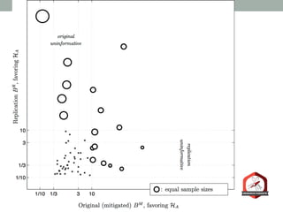
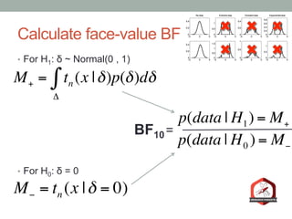
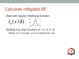
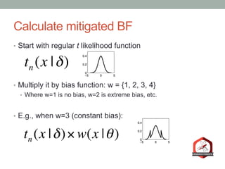
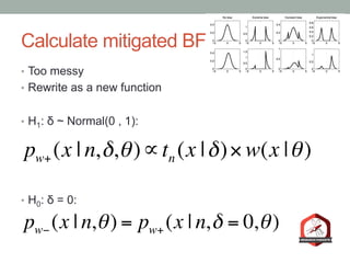
A Bayesian Perspective On
The Reproducibility Project:
Psychology
Alexander Etz & Joachim Vandekerckhove
@alxetz ßMy Twitter (no ‘e’ in alex)
alexanderetz.com ß My website/blog
Purpose
•  Revisit Reproducibility Project: Psychology (RPP)
•  Compute Bayes factors
•  Account for publication bias in original studies
•  Evaluate and compare levels of statistical evidence
TLDR: Conclusions first
•  75% of studies find qualitatively similar levels of evidence
in original and replication
•  64% find weak evidence (BF < 10) in both attempts
•  11% of studies find strong evidence (BF > 10) in both attempts
TLDR: Conclusions first
•  75% of studies find qualitatively similar levels of evidence
in original and replication
•  64% find weak evidence (BF < 10) in both attempts
•  11% of studies find strong evidence (BF > 10) in both attempts
•  10% find strong evidence in replication but not original
•  15% find strong evidence in original but not replication
The RPP
•  270 scientists attempt to closely replicate 100 psychology
studies
•  Use original materials (when possible)
•  Work with original authors
•  Pre-registered to avoid bias
•  Analysis plan specified in advance
•  Guaranteed to be published regardless of outcome
The RPP
•  2 main criteria for grading replication
The RPP
•  2 main criteria for grading replication
•  Is the replication result statistically significant (p < .05) in
the same direction as original?
•  39% success rate
The RPP
•  2 main criteria for grading replication
•  Is the replication result statistically significant (p < .05) in
the same direction as original?
•  39% success rate
•  Does the replication’s confidence interval capture original
reported effect?
•  47% success rate
The RPP
•  Neither of these metrics are any good
•  (at least not as used)
•  Neither make predictions about out-of-sample data
•  Comparing significance levels is bad
•  “The difference between significant and not significant is not
necessarily itself significant”
•  -Gelman & Stern (2006)
The RPP
•  Nevertheless, .51 correlation between original &
replication effect sizes
•  Indicates at least some level of robustness
−0.50
−0.25
0.00
0.25
0.50
0.75
1.00
0.00 0.25 0.50 0.75 1.00
Original Effect Size
ReplicationEffectSize
p−value
Not Significant
Significant
Replication Power
0.6
0.7
0.8
0.9
Source: Open Science Collaboration. (2015).
Estimating the reproducibility of psychological
science. Science, 349(6251), aac4716.
What can explain the discrepancies?
Moderators
•  Two study attempts are in different contexts
•  Texas vs. California
•  Different context = different results?
•  Conservative vs. Liberal sample
Low power in original studies
•  Statistical power:
•  The frequency with which a study will yield a statistically significant
effect in repeated sampling, assuming that the underlying effect is
of a given size.
•  Low powered designs undermine credibility of statistically
significant results
•  Button et al. (2013)
•  Type M / Type S errors (Gelman & Carlin, 2014)
Low power in original studies
•  Replications planned to have minimum 80% power
•  Report average power of 92%
Publication bias
•  Most published results are “positive” findings
•  Statistically significant results
•  Most studies designed to reject H0
•  Most published studies succeed
•  Selective preference = bias
•  “Statistical significance filter”
Statistical significance filter
•  Incentive to have results that reach p < .05
•  “Statistically significant”
•  Evidential standard
•  Studies with large effect size achieve significance
•  Get published
Statistical significance filter
•  Studies with smaller effect size don’t reach significance
•  Get suppressed
•  Average effect size inevitably inflates
•  Replication power calculations meaningless
Can we account for this bias?
•  Consider publication as part of data collection process
•  This enters through likelihood function
•  Data generating process
•  Sampling distribution
Mitigation of publication bias
•  Remember the statistical significance filter
•  We try to build a statistical model of it
Mitigation of publication bias
•  We formally model 4 possible significance filters
•  4 models comprise overall H0
•  4 models comprise overall H1
•  If result consistent with bias, then Bayes factor penalized
•  Raise the evidence bar
Mitigation of publication bias
•  Expected distribution of test statistics that make it to the
literature.
Mitigation of publication bias
•  None of these are probably right
•  (Definitely all wrong)
•  But it is a reasonable start
•  Doesn’t matter really
•  We’re going to mix and mash them all together
•  “Bayesian Model Averaging”
The Bayes Factor
•  How the data shift the balance of evidence
•  Ratio of predictive success of the models
BF10 =
p(data | H1)
p(data | H0 )
The Bayes Factor
•  H0: Null hypothesis
•  H1: Alternative hypothesis
BF10 =
p(data | H1)
p(data | H0 )
The Bayes Factor
•  BF10 > 1 means evidence favors H1
•  BF10 < 1 means evidence favors H0
•  Need to be clear what H0 and H1 represent
BF10 =
p(data | H1)
p(data | H0 )
The Bayes Factor
•  H0: d = 0
BF10 =
p(data | H1)
p(data | H0 )
The Bayes Factor
•  H0: d = 0
•  H1: d ≠ 0
BF10 =
p(data | H1)
p(data | H0 )
The Bayes Factor
•  H0: d = 0
•  H1: d ≠ 0 (BAD)
•  Too vague
•  Doesn’t make predictions
BF10 =
p(data | H1)
p(data | H0 )
The Bayes Factor
•  H0: d = 0
•  H1: d ~ Normal(0, 1)
•  The effect is probably small
•  Almost certainly -2 < d < 2”
BF10 =
p(data | H1)
p(data | H0 )
Statistical evidence
•  Do independent study attempts obtain similar amounts of
evidence?
Statistical evidence
•  Do independent study attempts obtain similar amounts of
evidence?
•  Same prior distribution for both attempts
•  Measuring general evidential content
•  We want to evaluate evidence from outsider perspective
Interpreting evidence
•  “How convincing would these data be to a neutral
observer?”
•  1:1 prior odds for H1 vs. H0
•  50% prior probability for each
Interpreting evidence
•  BF > 10 is sufficiently evidential
•  10:1 posterior odds for H1 vs. H0 (or vice versa)
•  91% posterior probability for H1 (or vice versa)
Interpreting evidence
•  BF > 10 is sufficiently evidential
•  10:1 posterior odds for H1 vs. H0 (or vice versa)
•  91% posterior probability for H1 (or vice versa)
•  BF of 3 is too weak
•  3:1 posterior odds for H1 vs. H0 (or vice versa)
•  Only 75% posterior probability for H1 (or vice versa)
Interpreting evidence
•  It depends on context (of course)
•  You can have higher or lower standards of evidence
Interpreting evidence
•  How do p values stack up?
•  American Statistical Association:
•  “Researchers should recognize that a p-value … near 0.05 taken
by itself offers only weak evidence against the null hypothesis. “
Interpreting evidence
•  How do p values stack up?
•  p < .05 is weak standard
•  p = .05 corresponds to BF ≤ 2.5 (at BEST)
•  p = .01 corresponds to BF ≤ 8 (at BEST)
Face-value BFs
•  Standard Bayes factor
•  Bias free
•  Results taken at face-value
Bias-mitigated BFs
•  Bayes factor accounting for possible bias
Illustrative Bayes factors
•  Study 27
•  t(31) = 2.27, p=.03
•  Maximum BF10 = 3.4
Illustrative Bayes factors
•  Study 27
•  t(31) = 2.27, p=.03
•  Maximum BF10 = 3.4
•  Face-value BF10 = 2.9
Illustrative Bayes factors
•  Study 27
•  t(31) = 2.27, p=.03
•  Maximum BF10 = 3.4
•  Face-value BF10 = 2.9
•  Bias-mitigated BF10 = .81
Illustrative Bayes factors
•  Study 71
•  t(373) = 4.4, p < .001
•  Maximum BF10 = ~2300
Illustrative Bayes factors
•  Study 71
•  t(373) = 4.4, p < .001
•  Maximum BF10 = ~2300
•  Face-value BF10 = 947
Illustrative Bayes factors
•  Study 71
•  t(373) = 4.4, p < .001
•  Maximum BF10 = ~2300
•  Face-value BF10 = 947
•  Bias-mitigated BF10 = 142
RPP Sample
•  N=72
•  All univariate tests (t test, anova w/ 1 model df, etc.)
Results
•  Original studies, face-value
•  Ignoring pub bias
•  43% obtain BF10 > 10
•  57% obtain 1/10 < BF10 < 10
•  0 obtain BF10 < 1/10
Results
•  Original studies, bias-corrected
•  26% obtain BF10 > 10
•  74% obtain 1/10 < BF10 < 10
•  0 obtain BF10 < 1/10
Results
•  Replication studies, face value
•  No chance for bias, no need for correction
•  21% obtain BF10 > 10
•  79% obtain 1/10 < BF10 < 10
•  0 obtain BF10 < 1/10
Consistency of results
•  No alarming inconsistencies
•  46 cases where both original and replication show only
weak evidence
•  Only 8 cases where both show BF10 > 10
Consistency of results
•  11 cases where original BF10 > 10, but not replication
•  7 cases where replication BF10 > 10, but not original
•  In every case, the study obtaining strong evidence had
the larger sample size
Moderators?
•  As Laplace would say, we have no need for that
hypothesis
•  Results adequately explained by:
•  Publication bias in original studies
•  Generally weak standards of evidence
Take home message
•  Recalibrate our intuitions about statistical evidence
•  Reevaluate expectations for replications
•  Given weak evidence in original studies
Thank you
Thank you
@alxetz ßMy Twitter (no ‘e’ in alex)
alexanderetz.com ß My website/blog
@VandekerckhoveJ ß Joachim’s Twitter
joachim.cidlab.com ß Joachim’s website
Want to learn more Bayes?
•  My blog:
•  alexanderetz.com/understanding-bayes
•  “How to become a Bayesian in eight easy steps”
•  http://tinyurl.com/eightstepsdraft
•  JASP summer workshop
•  https://jasp-stats.org/
•  Amsterdam, August 22-23, 2016
Technical Appendix
Mitigation of publication bias
•  Model 1: No bias
•  Every study has same chance of publication
•  Regular t distributions
•  H0 true: Central t
•  H0 false: Noncentral t
•  These are used in standard BFs
Mitigation of publication bias
•  Model 2: Extreme bias
•  Only statistically significant results published
•  t distributions but…
•  Zero density in the middle
•  Spikes in significant regions
Mitigation of publication bias
•  Model 3: Constant-bias
•  Nonsignificant results published x% as often as significant results
•  t distributions but…
•  Central regions downweighted
•  Large spikes over significance regions
Mitigation of publication bias
•  Model 4: Exponential bias
•  “Marginally significant” results have a chance to be published
•  Harder as p gets larger
•  t likelihoods but…
•  Spikes over significance regions
•  Quick decay to zero density as
(p – α) increases
Calculate face-value BF
•  Take the likelihood:
•  Integrate with respect to prior distribution, p(δ)
tn (x |δ)
Calculate face-value BF
•  Take the likelihood:
•  Integrate with respect to prior distribution, p(δ)
•  “What is the average likelihood of the data given this model?”
•  Result is marginal likelihood, M
tn (x |δ)
Calculate face-value BF
•  For H1: δ ~ Normal(0 , 1)
•  For H0: δ = 0
M− = tn (x |δ = 0)
M+ = tn (x |δ)
Δ
∫ p(δ)dδ
Calculate face-value BF
•  For H1: δ ~ Normal(0 , 1)
•  For H0: δ = 0
M− = tn (x |δ = 0)
M+ = tn (x |δ)
Δ
∫ p(δ)dδ
BF10=
p(data | H1) = M+
p(data | H0 ) = M−
Calculate mitigated BF
•  Start with regular t likelihood function
•  Multiply it by bias function: w = {1, 2, 3, 4}
•  Where w=1 is no bias, w=2 is extreme bias, etc.
tn (x |δ)
Calculate mitigated BF
•  Start with regular t likelihood function
•  Multiply it by bias function: w = {1, 2, 3, 4}
•  Where w=1 is no bias, w=2 is extreme bias, etc.
•  E.g., when w=3 (constant bias):
tn (x |δ)
tn (x |δ)× w(x |θ)
Calculate mitigated BF
•  Too messy
•  Rewrite as a new function
Calculate mitigated BF
•  Too messy
•  Rewrite as a new function
•  H1: δ ~ Normal(0 , 1):
pw+ (x | n,δ,θ)∝tn (x |δ)× w(x |θ)
Calculate mitigated BF
•  Too messy
•  Rewrite as a new function
•  H1: δ ~ Normal(0 , 1):
•  H0: δ = 0:
pw+ (x | n,δ,θ)∝tn (x |δ)× w(x |θ)
pw− (x | n,θ) = pw+ (x | n,δ = 0,θ)
Calculate mitigated BF
•  Integrate w.r.t. p(θ) and p(δ)
•  “What is the average likelihood of the data given each bias model?”
•  p(data | bias model w):
Calculate mitigated BF
•  Integrate w.r.t. p(θ) and p(δ)
•  “What is the average likelihood of the data given each bias model?”
•  p(data | bias model w):
Mw+ =
Δ
∫ pw+ (x | n,δ,θ)
Θ
∫ p(δ)p(θ)dδdθ
Calculate mitigated BF
•  Integrate w.r.t. p(θ) and p(δ)
•  “What is the average likelihood of the data given each bias model?”
•  p(data | bias model w):
Mw+ =
Δ
∫ pw+ (x | n,δ,θ)
Θ
∫ p(δ)p(θ)dδdθ
Mw− = pw− (x | n,θ)
Θ
∫ p(θ)dθ
Calculate mitigated BF
•  Take Mw+ and Mw- and multiply by the weights of the
corresponding bias model, then sum within each
hypothesis
Calculate mitigated BF
•  Take Mw+ and Mw- and multiply by the weights of the
corresponding bias model, then sum within each
hypothesis
•  For H1:
p(w =1)M1+ + p(w = 2)M2+ + p(w = 3)M3+ + p(w = 4)M4+
Calculate mitigated BF
•  Take Mw+ and Mw- and multiply by the weights of the
corresponding bias model, then sum within each
hypothesis
•  For H1:
•  For H0:
p(w =1)M1+ + p(w = 2)M2+ + p(w = 3)M3+ + p(w = 4)M4+
p(w =1)M1− + p(w = 2)M2− + p(w = 3)M3− + p(w = 4)M4−
Calculate mitigated BF
•  Messy, so we restate as sums:
Calculate mitigated BF
•  Messy, so we restate as sums:
•  For H1:
w
∑ p(w)Mw+
Calculate mitigated BF
•  Messy, so we restate as sums:
•  For H1:
•  For H0:
w
∑ p(w)Mw+
w
∑ p(w)Mw−
Calculate mitigated BF
•  Messy, so we restate as sums:
•  For H1:
BF10 =
•  For H0:
w
∑ p(w)Mw+
w
∑ p(w)Mw−
p(data | H1) =
w
∑ p(w)Mw+
p(data | H0 ) =
w
∑ p(w)Mw−

Bayes rpp bristol

  • 1.
    A Bayesian PerspectiveOn The Reproducibility Project: Psychology Alexander Etz & Joachim Vandekerckhove @alxetz ßMy Twitter (no ‘e’ in alex) alexanderetz.com ß My website/blog
  • 2.
    Purpose •  Revisit ReproducibilityProject: Psychology (RPP) •  Compute Bayes factors •  Account for publication bias in original studies •  Evaluate and compare levels of statistical evidence
  • 3.
    TLDR: Conclusions first • 75% of studies find qualitatively similar levels of evidence in original and replication •  64% find weak evidence (BF < 10) in both attempts •  11% of studies find strong evidence (BF > 10) in both attempts
  • 4.
    TLDR: Conclusions first • 75% of studies find qualitatively similar levels of evidence in original and replication •  64% find weak evidence (BF < 10) in both attempts •  11% of studies find strong evidence (BF > 10) in both attempts •  10% find strong evidence in replication but not original •  15% find strong evidence in original but not replication
  • 5.
    The RPP •  270scientists attempt to closely replicate 100 psychology studies •  Use original materials (when possible) •  Work with original authors •  Pre-registered to avoid bias •  Analysis plan specified in advance •  Guaranteed to be published regardless of outcome
  • 6.
    The RPP •  2main criteria for grading replication
  • 7.
    The RPP •  2main criteria for grading replication •  Is the replication result statistically significant (p < .05) in the same direction as original? •  39% success rate
  • 8.
    The RPP •  2main criteria for grading replication •  Is the replication result statistically significant (p < .05) in the same direction as original? •  39% success rate •  Does the replication’s confidence interval capture original reported effect? •  47% success rate
  • 9.
    The RPP •  Neitherof these metrics are any good •  (at least not as used) •  Neither make predictions about out-of-sample data •  Comparing significance levels is bad •  “The difference between significant and not significant is not necessarily itself significant” •  -Gelman & Stern (2006)
  • 10.
    The RPP •  Nevertheless,.51 correlation between original & replication effect sizes •  Indicates at least some level of robustness
  • 11.
    −0.50 −0.25 0.00 0.25 0.50 0.75 1.00 0.00 0.25 0.500.75 1.00 Original Effect Size ReplicationEffectSize p−value Not Significant Significant Replication Power 0.6 0.7 0.8 0.9 Source: Open Science Collaboration. (2015). Estimating the reproducibility of psychological science. Science, 349(6251), aac4716.
  • 12.
    What can explainthe discrepancies?
  • 13.
    Moderators •  Two studyattempts are in different contexts •  Texas vs. California •  Different context = different results? •  Conservative vs. Liberal sample
  • 14.
    Low power inoriginal studies •  Statistical power: •  The frequency with which a study will yield a statistically significant effect in repeated sampling, assuming that the underlying effect is of a given size. •  Low powered designs undermine credibility of statistically significant results •  Button et al. (2013) •  Type M / Type S errors (Gelman & Carlin, 2014)
  • 15.
    Low power inoriginal studies •  Replications planned to have minimum 80% power •  Report average power of 92%
  • 16.
    Publication bias •  Mostpublished results are “positive” findings •  Statistically significant results •  Most studies designed to reject H0 •  Most published studies succeed •  Selective preference = bias •  “Statistical significance filter”
  • 17.
    Statistical significance filter • Incentive to have results that reach p < .05 •  “Statistically significant” •  Evidential standard •  Studies with large effect size achieve significance •  Get published
  • 18.
    Statistical significance filter • Studies with smaller effect size don’t reach significance •  Get suppressed •  Average effect size inevitably inflates •  Replication power calculations meaningless
  • 19.
    Can we accountfor this bias? •  Consider publication as part of data collection process •  This enters through likelihood function •  Data generating process •  Sampling distribution
  • 20.
    Mitigation of publicationbias •  Remember the statistical significance filter •  We try to build a statistical model of it
  • 21.
    Mitigation of publicationbias •  We formally model 4 possible significance filters •  4 models comprise overall H0 •  4 models comprise overall H1 •  If result consistent with bias, then Bayes factor penalized •  Raise the evidence bar
  • 22.
    Mitigation of publicationbias •  Expected distribution of test statistics that make it to the literature.
  • 23.
    Mitigation of publicationbias •  None of these are probably right •  (Definitely all wrong) •  But it is a reasonable start •  Doesn’t matter really •  We’re going to mix and mash them all together •  “Bayesian Model Averaging”
  • 24.
    The Bayes Factor • How the data shift the balance of evidence •  Ratio of predictive success of the models BF10 = p(data | H1) p(data | H0 )
  • 25.
    The Bayes Factor • H0: Null hypothesis •  H1: Alternative hypothesis BF10 = p(data | H1) p(data | H0 )
  • 26.
    The Bayes Factor • BF10 > 1 means evidence favors H1 •  BF10 < 1 means evidence favors H0 •  Need to be clear what H0 and H1 represent BF10 = p(data | H1) p(data | H0 )
  • 27.
    The Bayes Factor • H0: d = 0 BF10 = p(data | H1) p(data | H0 )
  • 28.
    The Bayes Factor • H0: d = 0 •  H1: d ≠ 0 BF10 = p(data | H1) p(data | H0 )
  • 29.
    The Bayes Factor • H0: d = 0 •  H1: d ≠ 0 (BAD) •  Too vague •  Doesn’t make predictions BF10 = p(data | H1) p(data | H0 )
  • 30.
    The Bayes Factor • H0: d = 0 •  H1: d ~ Normal(0, 1) •  The effect is probably small •  Almost certainly -2 < d < 2” BF10 = p(data | H1) p(data | H0 )
  • 31.
    Statistical evidence •  Doindependent study attempts obtain similar amounts of evidence?
  • 32.
    Statistical evidence •  Doindependent study attempts obtain similar amounts of evidence? •  Same prior distribution for both attempts •  Measuring general evidential content •  We want to evaluate evidence from outsider perspective
  • 33.
    Interpreting evidence •  “Howconvincing would these data be to a neutral observer?” •  1:1 prior odds for H1 vs. H0 •  50% prior probability for each
  • 34.
    Interpreting evidence •  BF> 10 is sufficiently evidential •  10:1 posterior odds for H1 vs. H0 (or vice versa) •  91% posterior probability for H1 (or vice versa)
  • 35.
    Interpreting evidence •  BF> 10 is sufficiently evidential •  10:1 posterior odds for H1 vs. H0 (or vice versa) •  91% posterior probability for H1 (or vice versa) •  BF of 3 is too weak •  3:1 posterior odds for H1 vs. H0 (or vice versa) •  Only 75% posterior probability for H1 (or vice versa)
  • 36.
    Interpreting evidence •  Itdepends on context (of course) •  You can have higher or lower standards of evidence
  • 37.
    Interpreting evidence •  Howdo p values stack up? •  American Statistical Association: •  “Researchers should recognize that a p-value … near 0.05 taken by itself offers only weak evidence against the null hypothesis. “
  • 38.
    Interpreting evidence •  Howdo p values stack up? •  p < .05 is weak standard •  p = .05 corresponds to BF ≤ 2.5 (at BEST) •  p = .01 corresponds to BF ≤ 8 (at BEST)
  • 39.
    Face-value BFs •  StandardBayes factor •  Bias free •  Results taken at face-value
  • 40.
    Bias-mitigated BFs •  Bayesfactor accounting for possible bias
  • 41.
    Illustrative Bayes factors • Study 27 •  t(31) = 2.27, p=.03 •  Maximum BF10 = 3.4
  • 42.
    Illustrative Bayes factors • Study 27 •  t(31) = 2.27, p=.03 •  Maximum BF10 = 3.4 •  Face-value BF10 = 2.9
  • 43.
    Illustrative Bayes factors • Study 27 •  t(31) = 2.27, p=.03 •  Maximum BF10 = 3.4 •  Face-value BF10 = 2.9 •  Bias-mitigated BF10 = .81
  • 44.
    Illustrative Bayes factors • Study 71 •  t(373) = 4.4, p < .001 •  Maximum BF10 = ~2300
  • 45.
    Illustrative Bayes factors • Study 71 •  t(373) = 4.4, p < .001 •  Maximum BF10 = ~2300 •  Face-value BF10 = 947
  • 46.
    Illustrative Bayes factors • Study 71 •  t(373) = 4.4, p < .001 •  Maximum BF10 = ~2300 •  Face-value BF10 = 947 •  Bias-mitigated BF10 = 142
  • 47.
    RPP Sample •  N=72 • All univariate tests (t test, anova w/ 1 model df, etc.)
  • 48.
    Results •  Original studies,face-value •  Ignoring pub bias •  43% obtain BF10 > 10 •  57% obtain 1/10 < BF10 < 10 •  0 obtain BF10 < 1/10
  • 49.
    Results •  Original studies,bias-corrected •  26% obtain BF10 > 10 •  74% obtain 1/10 < BF10 < 10 •  0 obtain BF10 < 1/10
  • 50.
    Results •  Replication studies,face value •  No chance for bias, no need for correction •  21% obtain BF10 > 10 •  79% obtain 1/10 < BF10 < 10 •  0 obtain BF10 < 1/10
  • 52.
    Consistency of results • No alarming inconsistencies •  46 cases where both original and replication show only weak evidence •  Only 8 cases where both show BF10 > 10
  • 53.
    Consistency of results • 11 cases where original BF10 > 10, but not replication •  7 cases where replication BF10 > 10, but not original •  In every case, the study obtaining strong evidence had the larger sample size
  • 55.
    Moderators? •  As Laplacewould say, we have no need for that hypothesis •  Results adequately explained by: •  Publication bias in original studies •  Generally weak standards of evidence
  • 56.
    Take home message • Recalibrate our intuitions about statistical evidence •  Reevaluate expectations for replications •  Given weak evidence in original studies
  • 57.
  • 58.
    Thank you @alxetz ßMyTwitter (no ‘e’ in alex) alexanderetz.com ß My website/blog @VandekerckhoveJ ß Joachim’s Twitter joachim.cidlab.com ß Joachim’s website
  • 59.
    Want to learnmore Bayes? •  My blog: •  alexanderetz.com/understanding-bayes •  “How to become a Bayesian in eight easy steps” •  http://tinyurl.com/eightstepsdraft •  JASP summer workshop •  https://jasp-stats.org/ •  Amsterdam, August 22-23, 2016
  • 60.
  • 61.
    Mitigation of publicationbias •  Model 1: No bias •  Every study has same chance of publication •  Regular t distributions •  H0 true: Central t •  H0 false: Noncentral t •  These are used in standard BFs
  • 62.
    Mitigation of publicationbias •  Model 2: Extreme bias •  Only statistically significant results published •  t distributions but… •  Zero density in the middle •  Spikes in significant regions
  • 63.
    Mitigation of publicationbias •  Model 3: Constant-bias •  Nonsignificant results published x% as often as significant results •  t distributions but… •  Central regions downweighted •  Large spikes over significance regions
  • 64.
    Mitigation of publicationbias •  Model 4: Exponential bias •  “Marginally significant” results have a chance to be published •  Harder as p gets larger •  t likelihoods but… •  Spikes over significance regions •  Quick decay to zero density as (p – α) increases
  • 65.
    Calculate face-value BF • Take the likelihood: •  Integrate with respect to prior distribution, p(δ) tn (x |δ)
  • 66.
    Calculate face-value BF • Take the likelihood: •  Integrate with respect to prior distribution, p(δ) •  “What is the average likelihood of the data given this model?” •  Result is marginal likelihood, M tn (x |δ)
  • 67.
    Calculate face-value BF • For H1: δ ~ Normal(0 , 1) •  For H0: δ = 0 M− = tn (x |δ = 0) M+ = tn (x |δ) Δ ∫ p(δ)dδ
  • 68.
    Calculate face-value BF • For H1: δ ~ Normal(0 , 1) •  For H0: δ = 0 M− = tn (x |δ = 0) M+ = tn (x |δ) Δ ∫ p(δ)dδ BF10= p(data | H1) = M+ p(data | H0 ) = M−
  • 69.
    Calculate mitigated BF • Start with regular t likelihood function •  Multiply it by bias function: w = {1, 2, 3, 4} •  Where w=1 is no bias, w=2 is extreme bias, etc. tn (x |δ)
  • 70.
    Calculate mitigated BF • Start with regular t likelihood function •  Multiply it by bias function: w = {1, 2, 3, 4} •  Where w=1 is no bias, w=2 is extreme bias, etc. •  E.g., when w=3 (constant bias): tn (x |δ) tn (x |δ)× w(x |θ)
  • 71.
    Calculate mitigated BF • Too messy •  Rewrite as a new function
  • 72.
    Calculate mitigated BF • Too messy •  Rewrite as a new function •  H1: δ ~ Normal(0 , 1): pw+ (x | n,δ,θ)∝tn (x |δ)× w(x |θ)
  • 73.
    Calculate mitigated BF • Too messy •  Rewrite as a new function •  H1: δ ~ Normal(0 , 1): •  H0: δ = 0: pw+ (x | n,δ,θ)∝tn (x |δ)× w(x |θ) pw− (x | n,θ) = pw+ (x | n,δ = 0,θ)
  • 74.
    Calculate mitigated BF • Integrate w.r.t. p(θ) and p(δ) •  “What is the average likelihood of the data given each bias model?” •  p(data | bias model w):
  • 75.
    Calculate mitigated BF • Integrate w.r.t. p(θ) and p(δ) •  “What is the average likelihood of the data given each bias model?” •  p(data | bias model w): Mw+ = Δ ∫ pw+ (x | n,δ,θ) Θ ∫ p(δ)p(θ)dδdθ
  • 76.
    Calculate mitigated BF • Integrate w.r.t. p(θ) and p(δ) •  “What is the average likelihood of the data given each bias model?” •  p(data | bias model w): Mw+ = Δ ∫ pw+ (x | n,δ,θ) Θ ∫ p(δ)p(θ)dδdθ Mw− = pw− (x | n,θ) Θ ∫ p(θ)dθ
  • 77.
    Calculate mitigated BF • Take Mw+ and Mw- and multiply by the weights of the corresponding bias model, then sum within each hypothesis
  • 78.
    Calculate mitigated BF • Take Mw+ and Mw- and multiply by the weights of the corresponding bias model, then sum within each hypothesis •  For H1: p(w =1)M1+ + p(w = 2)M2+ + p(w = 3)M3+ + p(w = 4)M4+
  • 79.
    Calculate mitigated BF • Take Mw+ and Mw- and multiply by the weights of the corresponding bias model, then sum within each hypothesis •  For H1: •  For H0: p(w =1)M1+ + p(w = 2)M2+ + p(w = 3)M3+ + p(w = 4)M4+ p(w =1)M1− + p(w = 2)M2− + p(w = 3)M3− + p(w = 4)M4−
  • 80.
    Calculate mitigated BF • Messy, so we restate as sums:
  • 81.
    Calculate mitigated BF • Messy, so we restate as sums: •  For H1: w ∑ p(w)Mw+
  • 82.
    Calculate mitigated BF • Messy, so we restate as sums: •  For H1: •  For H0: w ∑ p(w)Mw+ w ∑ p(w)Mw−
  • 83.
    Calculate mitigated BF • Messy, so we restate as sums: •  For H1: BF10 = •  For H0: w ∑ p(w)Mw+ w ∑ p(w)Mw− p(data | H1) = w ∑ p(w)Mw+ p(data | H0 ) = w ∑ p(w)Mw−