Approximating_probability_density_functions_for_the_Collective_Risk_Model

of 38
Approximating probability density functions for the
Collective Risk Model.
Harini Vaidyanath
Problem Report
Submitted to
West Virginia University
in partial fulfillment of the requirements
for the degree of
Master of Science
in
Statistics
Committee:
Robert Mnatsakanov, Ph. D., Chair
Erdogan Gunel, Ph. D.
E. James Harner, Ph. D.
Department of Statistics
Morgantown, West Virginia
May 2012

of 38
Acknowledgements:
I wish to thank Dr. Robert Mnatsakanov, Dr. Erdogan Gunel and Dr. Jim Harner for their
support and guidance.

of 38
Contents
TOPIC Page
1. INTRODUCTION 5
2. RISK THEORY 5
a. Major areas of risk theory. 6
b. How does Insurance work? 6
c. Sources of uncertainty for the insurer. 6
d. Distributions used in insurance claims modeling. 6
e. Studying aggregate claims distributions using sums of random
variables. 7
3. METHODS OF OBTAINING THE PROBABILITY FUNCTION FOR SN 7
a. The moment generating function method. 8
b. The direct convolution of distributions method. 8
c. Recursive calculation for discrete random variables. 9
4. THE COLLECTIVE RISK MODEL 11
a. The model. 11
b. The distribution of SN. 12
c. The probability function of SN. 13
5. RECURSIVE CALCULATION OF AGGREGATE CLAIMS
DISTRIBUTION 13
a. The (a, b, 0) class of distributions 13
i. The Panjer Recursion Formula 16
ii. Worked example 1 18
iii. Probability function of SN 18
iv. Visual representation of solution 19
v. Interpretation of graphs 19
b. The (a, b, 1) class of distributions 20
i. Extending the Panjer Recursion Formula 20

of 38
c. Schröter’s class of distributions 23
i. Other classes of distributions 23
d. Numerical Issues of using recursive techniques 28
e. Discretization process for continuous claim distributions 30
6. APPROXIMATION OF PROBABILITY FUNTION OF ‘S’: 31
a. Normal Approximation 31
b. Translated Gamma Approximation 31
c. Graphical comparison of solutions from Panjer Recursion, Normal
approximation and Translated Gamma Approximation 32
d. Interpretation of comparison
7. DISCUSSION AND CONCLUSION 34
8. REFERENCES 35
9. ‘R’ Codes 36

of 38
1
Introduction:
The topic of this project report is Approximating probability functions for the Collective
Risk Model with specific emphasis on using recursion techniques for obtaining the
probability functions.
Risk theory is studied to understand its uses in Insurance claims modeling. The Collective
Risk Model and the different methods of obtaining probability functions for the aggregate
claims from a collective risk portfolio are also studied. Obtaining these probability
functions can be of great interest to Insurance companies that are interested in
approximating the probability of occurrence of a certain aggregate claim size from a
portfolio.
Importance is given to using recursive techniques to compute probability functions
because of its ease of use in a programming environment.
Most of the content in this project report was learned from the text book – Insurance,
Risk, and Ruin by David C. M. Dickson and hence not many references are cited.
The Statistical Programming language ‘R’ was used both to compute values for the
probability functions and produce graphs.
2
Risk Theory:
Risk theory is a field studied by Actuaries and Insurers to understand the financial impact
of a loss on a carrier of a portfolio of insurance policies and to make decisions in the face
of uncertainty.
Risk theory can be identified with Insurance Risk Theory or with applying the theory of
probability to study problems arising in the Insurance field.
Modeling the distribution of claims from an insurer’s portfolio is a difficult task,
especially when the claims are from the non-life or general insurance policies. This is
because the models involve many random processes such as claim arrivals, claim
frequencies, claim severities, etc. It is important to note that since only claim frequencies

of 38
and sizes are considered when modeling claims from a portfolio, and since claim cause is
ignored, it is possible to assume that the claim sizes are IID random variables.
2.a
Major areas of Risk Theory:
There are two major areas in the field one of which is Risk Models for aggregate claims,
which the topic of my project report and the other is Ruin Theory.
2.b
How does Insurance work?
What is the typical operation of a motor vehicle insurance policy (a type of general
insurance policy) from an insurer’s point of view?
General insurance risks consist of risks from motor vehicle insurance, home and contents
insurance and travel insurance. Under motor vehicle policies, the insured party pays a
certain amount of money to the insurer to be covered against a pre specified set of losses
that they may incur in the event of an accident. This premium is paid at the start of the
period of insurance cover which is assumed to be one year. The insured party can make
claims each time an accident occurs resulting in damage to the vehicle hence requiring
repair costs.
2.c
Sources of uncertainty for the Insurer:
There are two sources of uncertainty for the insurer. One is the frequency of claims and
the other is the subsequent size of claims. So a probabilistic model representing the
claims outgoing under a policy would have to incorporate both these components. This is
also the general framework for modeling claims outgoing from any general insurance
policy.
2.d
Distributions used in insurance claims modeling:
Most of the distributions used to models claims model either the number of claims or the
size of individual claims. Mixed distributions can be used to model both the number of

of 38
claims and the size of individual claims and are especially useful in situations where there
are claims of size 0 (leading to unrealistic claim number estimates) or where claims size
exceed a certain set threshold amount that the company may possess in the form of
surplus (requiring the insurance company to resort to reinsurance).
An important and interesting problem in risk modeling is modeling aggregate claims, i.e.
finding the distribution of a sum of independent and identically distributed claim sizes
where claim sizes are treated as IID random variables.
Important discrete distributions used in risk modeling:
 The Poisson Distribution
 The Binomial Distribution
 The Negative Binomial Distribution
 The Geometric Distribution
Important continuous distributions used in risk modeling:
 The Gamma distribution
 The Exponential distribution
 The Pareto distribution
 The Normal Distribution
 The Log-normal Distribution
2.e
Studying Aggregate claims distribution using sums of random
variables:
Many modeling problems in the insurance industry are concerned with modeling
aggregate claims to find their distribution.
For example, if the company issues n policies, and the claim amount from policy i can be
represented as Xi, i = 1, 2, 3 … n, where the Xi are assumed to be IID, then, Sn = ∑
would represent the total amount the insurer would expect to pay as reimbursements
towards these n claims. The behavior of Sn is of interest to many insurance companies
and can be studied if the distribution is known. In many cases the distribution function
may not be very obvious and they need to be estimated or approximated using existing

of 38
distribution functions. Since the claims are assumed to be IID random variables, a variety
of methods can be used to obtain their distribution function.
3
Methods of obtaining the distribution function of Sn:
 Moment generating function method.
 Direct convolution of distributions.
 Recursive calculation for discrete random variables.
3.a
The Moment Generating Function (MGF) method:
This is a relatively simple way of finding the distribution of Sn, for fixed values of n,
where Ms can be defined as the MGF of Sn and Mx can be defined as the MGF function of
Xi.
Then it can be seen that
Ms(t) = E[et(Sn)
] = E[et(X1 + X2 + … Xn)
]
= E[et(X1)
] E[et(X2)
]∙∙∙ E[et(Xn)
] (Since the Xi are independent)
= [Mx(t)]n
(Since the Xi are identically distributed)
So, if Mx(t) can be identified as the MGF of a distribution, the distribution of Sn can be
identified using the uniqueness property of MGFs.
3.b
Direct convolutions of distributions:
Direct convolution is a more direct method of finding the distribution of Sn. Here, the
{Xi}, i = 1, 2, 3, ... ∞, are assumed to be discrete random variables, distributed on non-
negative integers so that Sn is also distributed on non-negative integers.
The distribution of S2 can be found using the convolution approach as follows. For this,
let us consider how the event {S2 ≤ x} can occur. It can occur when X2 takes the value j,

of 38
where j can take any value from 0 up to x, and when X1 take a value less than or equal to x
– j such that their sum is less than or equal to x.
Now, given that X1 and X2 are independent and summing over all possible values of j, it
can be seen that
Pr(S2 ≤ x) = ∑
Pr(S3 ≤ x) can be found using the same argument as above and in general it can be seen
that
Pr(Sn ≤ x) = ∑
From this, it is very easy to see
Pr(Sn = x) = ∑
Let’s define F to be the distribution function of X1 and let fj be its probability function
defined as Pr(X1 = j). Now, let’s call Fn*
the n-fold convolution of the distribution F with
itself. Then from the results above it follows that
Fn*
(x) = ∑ fj(x)
Note that F1*
= F, and, define F0*
(x) = {
Similarly, define fx
n*
= Pr(Sn = x) so that fx
n*
= ∑ fj with f1*
= f.
When F is continuous on (0,∞), the analogues of the above results are
Fn*
(x) = ∫ F(n-1)*
(x-y) f(y) dy
and
fn*
(x) = ∫ f(n-1)*
(x-y) f(y) dy
Using these results, it is easy to find the distribution and hence probability function of Sn
directly.

of 38
3.c
Recursive calculation for discrete random variables:
When the Xi are discrete random variables distributed on non-negative integers, the
probability function of Sn can be calculated recursively.
Let us use the following notation
fj = Pr(X1 = j) and gj = Pr(Sn = j) for j = 0,1,2,…
Before we move on any further, let’s define what a probability generating function is.
The probability generating function of a discrete random variable is a power series
representation of the probability mass function of the random variable.
Let us denote the probability generating function of X1 by Px and that of Sn to be PS.
Let them be defined as
PX(r) = ∑ fj
and
PS(r) = ∑ gk
From the results derived for moment generating functions, it can be easily seen that
PS(r) = [PX(r)]n
Differentiating the above result with respect to r and multiplying throughout by rPX(r)
gives
r PX(r) P′S(r) = n r PS(r)P′X(r)
Substituting the respective probability generating functions into the above equations, we
have
∑ fj ∑ gk = n ∑ gk ∑ fj
Since the goal is to find an expression for gx, start by considering the coefficient of rx
on
each side of the above equation.

of 38
The coefficient of rx
is obtained from the above equation by multiplying the coefficient of
rj
in the first sum, with the coefficient of rx-j
in the second sum, f or j = 0, 1, 2, …, x-1,.
Adding these products we get the coefficient of rx
from the left hand side of the equation
as
f0xgx + f1(x-1)gx-1 + … + fr-1g1 = ∑ (x-j) fjgx-j
and from the right hand side of the equation as
n(g0xfx + g1(x-1)fx-1 + … + gx-1f1) = n∑ jfjgx-j
Equating these coefficients, it can be seen that
xgxf0 + ∑ (x-j)fjgx-j = n∑ jfjgx-j
from which it can be seen that (noting that the sum on the left hand side is unaltered when
the upper limit of the sum is increased to x)
gx = ∑ ((n+1) – 1) fjgx-j
The above equation can be used recursively to obtain values of gx for x = 0, 1, 2, 3, … ∞
Using the values of fj, j = 0, 1, 2, 3, …, ∞, it is possible to calculate g1 using g0, and g2
using g0, g1, and so on. The starting value for gx namely g0 is given by
Pr(Sn = 0) = Pr(∑ = 0) = ∏ = [Pr(Xi = 0)]n
= f0
n
.
The form of gx obtained in the above result is very useful as it permits a much more
efficient evaluation of the probability function of Sn than the direct convolution method.
Now that we have had an introduction to the distributions frequently used in risk
modeling and the different methods of obtaining them, let us move on to the kinds of
models used.
The models are of two kinds, The Collective Risk model and The Individual Risk Model.
My research focuses on The Collective Risk Model, with specific emphasis on using
recursive techniques for computing the probability function of aggregate claims when the
individual claim probability function is specified and distributed on non-negative
integers.

of 38
4
The Collective Risk Model
Let’s consider the aggregate claims arising from a general insurance risk over a short
period of time, say one year (although any unit of time can be considered). The term
‘risk’ is used here to describe either a collection of similar policies or an individual policy
in a portfolio. Many times this setup may be referred to as a risk portfolio.
It is important to note that at the start of the period of an insurance cover, the insurer
knows neither the number of claims that may occur, nor the size of the claims. So, when
constructing a model, it is important to take into account these two sources of variability.
4.a
The model:
Let’s denote the aggregate (i.e. total) claims random variable by S for the modeling
process. A risk portfolio is a collection of Insurance policies that have been issued by a
company. N denotes the random number of claims arising from this risk portfolio and Xi
denotes the size of the ith
claim.
The aggregate claim amount is then, just the sum of the individual claim amounts and is
given by
S = ∑
noting that S = 0 when N = 0, i.e. the aggregate claim amount is 0 when there are no
claims. It is also important to note that individual claim amounts are modeled as non –
negative random variables with positive mean.
There are two important assumptions that need to be made when modeling aggregate
claims. The first assumption is that the claim size random variables {Xi}, i = 1, 2, 3, … ∞
are independent of each other and identically distributed throughout the year. The second
assumption is that the number of claims N is independent of the claims size.
The name collective risk model is used to denote the fact that the risk is being considered
as a whole i.e. we count the number of claims from the portfolio as a whole and not from
individual policies.

of 38
4.b
The distribution of S:
Let us denote the distribution functions of S and X1 as G and F respectively with
G(x) = Pr(S ≤ x) and F(x) = Pr(X1 ≤ x)
Let {pn}, n = 1, 2, 3, … ∞ denote the probability function of the number of claims with
pn = Pr(N=n)
G can then be derived as follows. The event {S ≤ x} can occur if n claims occur and the
sum of these claims is no more than x. The event {S ≤ x} can also be represented as the
union of two mutually exclusive events {S ≤ x and N = n} i.e.
{S ≤ x} = ⋃
Then,
G(x) = Pr(S ≤ x) = Pr(⋃ )
= ∑
Now,
Pr(S ≤ x and N = n) = Pr(S ≤ x | N = n) Pr(N = n)
and by definition,
Pr(S ≤ x and N = n) Pr(∑ ≤ x ) = Fn*
(x)
So, for x ≥ 0, we have
G(x) = ∑ pn
where F0*
(x) = 1 for x ≥ 0, and 0 otherwise.

of 38
4.c
The probability function of Sn:
When individual claim amounts are distributed on positive integers, the probability
function is given by
fj = F(j) – F(j-1) where j = 1,2,3,…
and using this, the probability mass function, corresponding to G(x) is
gx = ∑ pn f n*
for x = 1, 2, 3, …
where f n*
= Pr(∑ = x) and g0 = p0.
The formulae above can be used to calculate gx for x = 0, 1, 2, … recursively when N
follows certain pre specified distributions.
5
Recursive calculation of aggregate claims distributions:
Recursive calculation of aggregate claims distributions is possible when claim amounts
are distributed on non-negative integers and when claim number distribution (a.k.a the
counting distribution) belongs to the (a, b, 0) class of distributions.
5.a
The (a, b, 0) class of distributions:
A counting distribution belongs to the (a, b, 0) class of distributions if its probability
function can be calculated recursively using the formula
pn = (a + ) pn-1 for n = 1, 2, 3, …, where a and b are constants.
The starting value for the calculation is p0 ≥ 0 and the term 0 in (a, b, 0) is used to
indicate this fact.

of 38
What distributions belong to the (a, b, 0) class?
There are 3 non-trivial distributions that belong to the (a, b, 0) class and they are
 The Poisson Distribution
 The Binomial Distribution
 The Negative Binomial Distribution
Members of the (a, b, 0) class can be identified by considering values for a, b as follows.
It can be seen that the recursion formula starts from and satisfies
p1 = (a + b) p0
This requires a+b ≥ 0 for pn to be positive.
Case 1:
Let a + b = 0. Then pn = 0 for n = 1, 2, 3… By definition of a probability function, we
know that ∑ = 1and hence, p0 must be 1 making the distribution degenerate at 0.
Case 2:
Let a = 0. This gives pn = pn-1 for n = 1, 2, 3, … so that
pn = ∙∙∙ b p0
= p0
Using the fact that ∑ = 1, it can be seen that
∑ = p0 ∑ = p0 eb
= 1
giving p0 = e –b
which is a Poisson distribution with mean b.
Case 3:
Let a > 0 and a ≠ - b so that a + b > 0. Then, by applying the formula of pn repeatedly,
we have
pn = (n + ) (n-1 + ) ∙∙∙ (2 + ) (1 + ) p0

of 38
If we let α denote 1 + , the above equation becomes
pn = (n-1-α) (n-2-α) ∙∙∙ (1+α) α p0
= ( –
) an
p0
To identify this distribution, note that as p0 > 0, we require ∑ < 1.
By d’Alembert’s ratio test‡
, we have absolute convergence if
Limit | | < 1
and as pn = (a + )pn-1, we have absolute convergence if |a| < 1. Since a > 0, this
condition reduces to a < 1.
Then
∑ = p0 + p0 ∑ ( –
) an
= 1.
From the definition of the probability function for NB(k, p) we have
pk
∑ ( –
) qn
= 1 - pk
with p + q = 1
Hence p0 = (1-a)α
and the distribution of N of negative binomial with parameters k = 1 –
a, where 0 < a < 1, and α = 1 + .
Case 4:
Let a + b > 0 and a < 0. As a < 0, there must exist a positive integer χ such that
a + = 0
so that pn = 0, n = χ +1, χ +2, …. for pn to have non-negative values.
Proceeding as above, we have
‡
In mathematics, the d’Alembert’s ratio test is a test for the convergence of a series ∑ , when each term is a real or
complex number and is nonzero when n is very large.

of 38
pn = (-a)n
( )p0
Since we have assumed that a < 0, let A = -a >0. Then,
∑ = p0 ∑ ( )An
= p0 ∑ ( )An
= 1
To find p0 we can write A = which is equivalent to writing p = = so that 0 < p
< 1. Then
p0∑ ( )pn
(1-p)-n
= 1
which gives p0 = (1-p)χ
, and the distribution of N is binomial with parameters χ and
These parameters for distributions belonging to the (a, b, 0) class can be tabulated as
follows:
a b
P(λ) 0 λ
B(n,q)
NB(k,p) 1-p (1-p)(k-1)
An important result from page 67 of the book Insurance, Risk, and Ruin that will be
applied later is
P′N(r) = ar P′N(r) + (a+b) PN(r) --- (†)
5.a.i
The Panjer Recursion formula:
The Panjer recursion formula is one of the most important results in risk theory. This
recursion formula allows us to calculate the probability function of aggregate claims
when the counting distribution belong to the (a, b, 0) class and when the individual claim
amount distribution is discrete with probability function fj. It is useful to allow f0 > 0 even
though in practice, an individual claim amount of zero would not constitute a claim. This

of 38
is especially useful in the discretization process of continuous claims, which is a
technique used to discretize continuous distributions.
For the moment, since individual claim amounts are assumed to be distributed on non-
negative integers, it follows that S is also distributed on non-negative integers. There are
two ways in which aggregate claims are of size zero. The first is when there are no
claims, i.e. N = 0 and the second is when there are n claims and each claim is of size zero
i.e. Xi for each i = 1, 2, 3, …
Let’s discard the case where N = 0 and consider the case when each claim is of size zero
i.e. ∑ = 0. Since independence of claims have been assumed, we have
Pr(∑ = 0) = ∏
= ∏
=
From the definition of gx, we can define g0, the initial value for the recursion as,
g0 = p0 + ∑
= PN(f0)
Now, the probability generating function of S is given by
PS(r) = PN[PX(r)]
and differentiating the above with respect to r gives,
P′S(r) = P′N[PX(r)]P′X(r)
From (†), it follows that
P′S(r) = (aPX(r)P′N[PX(r)] + (a+b)PN[PX(r)]) P′X(r)
= aPX(r)P′S(r) + (a+b)PS(r)P′X(r)
Substituting definitions for probability generating functions and rearranging terms of the
resulting equation, the probability function of S is found to be
gx = ∑ fk gx-k

of 38
and this is the Panjer recursion formula. One the advantage that this formula has over the
one derived earlier is that this is more efficient from a computational point of view.
5.a.i
Worked Example 1:
Let N ~ P(2), and let fj = 0.6(0.4 j-1
) for j = 1, 2, 3, … Calculate gx for x = 0, 1, 2, ….
Solution:
 f0 = 0
 g0 = p0
 a = 0
 b = 0
5.a.ii
Probability function of SN:
gx = ∑ fk gx-k
= ∑ k fk gx-k
Using the above information, we have
 Pr(S = 0) = g0 = e-2
 Pr(S = 1) = g1 = 2f1g0 = 0.1624
 Pr(S = 2) = g2 = f1g1 + 2f2g0 = 0.1624
 Pr(S = 3) = g3 = (f1g2 + 2f2g1 + 3f3g0) = 0.1429
 …

of 38
5.a.iv
Visual representation of solution:
5.a.v
Interpretation of graphs:
It is seen that both the individual and aggregate claims mass functions are positively
skewed and it can be inferred that small claim sizes have a high probability of occurring.
It is seen that about 60% of the claims are of size 1 unit, 25% of size 2 units, and 10% of
size 3 units and so on. The probabilities of the claim sizes being less than or equal to a
certain value x can be computed by summing the probability mass functions for values of
X ≤ x, i.e. it can be seen that less than 2% of the claim are of size greater than or equal to
5 units and the probability of claims taking values of 6 units or more are almost
negligible. Probabilities of claims lying within a certain range for x can also be calculated
easily. Similar results can be obtained from the graph for the aggregate claims. It is
important to note that the mass functions of aggregate claims are almost always
positively skewed. This result would be great interest to insurance companies since most
are profit oriented organizations and would like to insure risks with low probabilities of
occurrences.

of 38
5.b
The (a, b, 1) class of distributions:
5.b.i
Extending the Panjer Recursion Formula:
A counting distribution is said to belong to the (a, b, 1) class of distributions, if its
probability function {qn}, n = 1, 2, 3, … ∞, can be computed recursively from the
formula
qn = (a + ) qn-1
for n = 2, 3, 4, … where a and b are constants. This class differs from the (a, b, 0) class
because the starting value for the recursive calculation is q1 which is assumed to be
greater than 0 and the term ‘1’ in the (a, b, 1) is used to indicate the starting point for the
recursion.
As the basic recursion formula is the same for both the classes, the members of the (a, b,
1) class can be constructed by modifying the mass of probability at 0 in the distributions
of the (a, b, 0) class. This modification can be done in two ways. The first method of
modification is called zero-truncation and the second method is called zero-modification.
Zero-Truncation Method:
Let {pn}, n = 1, 2, 3, .. ∞ be a probability function in the (a, b, 0) class. It’s zero-truncated
counterpart is given by
qn =
for n = 1, 2, 3, ….
For example, the zero-truncated Poisson distribution with parameter λ is given by
qn =
for n = 1, 2, 3, …

of 38
Zero-Modification Method:
Let {pn}, n = 1, 2, 3, … ∞, be a probability function in the (a, b, 0) class. It’s zero
modified counterpart is given by q0 = α where 0 < α < 1, n = 0, and for n = 1, 2, 3,..,
qn = ( ) pn
So, the probability p0 in the (a, b, 0) class is being replaced by α and the remaining
probabilities are being rescaled.
For example, the zero-modified geometric distribution with pn = pqn
for n = 0, 1, 2, … is
given by q0 = α for n = 0 and for n = 1, 2, 3, … by
qn = ) pqn
= (1- α)pqn-1
There are four members in the (a, b, 1) class. Two of them are the logarithmic
distribution and the extended truncated negative binomial distribution. The other two are
their respective zero-modified versions.
When the counting distributions belong to the (a, b, 1) class and individual claim
amounts are distributed on the non-negative integers, the techniques discussed previously
can be used to derive a recursion formula for the probability function of the aggregate
claims and its final form is given by
gx = [ ∑ fj gx-j + (q1 – (a+b)q0)fx ]
for x = 1, 2, 3, …and the starting value for this recursion formula is
g0 = ∑ qn = QN(f0)
when f0 > 0. When f0 = 0and q0 > 0, the starting value for this recursion formula is simply
g0 = q0 and when both q0 and f0 are 0, the starting value is
g1 = Pr(N=1)Pr(X1=1) = q1f1
5.b.ii
Worked Example 2:
Let N have a logarithmic distribution with parameter θ = 0.5, and let f1 = 0.2(0.8j-1
) for j =
0, 1, 2, 3, … Compute gx for x = 0, 1, 2, …

of 38
Solution:
The logarithmic probability function is
qn =
for n = 1, 2, 3, …
Let us note the following information
 q1 = 0.7213
 a = θ = 0.5
 b = - θ = - 0.5
 f0 = 0.2
 QN(r) =
 Pr(S = 0) = g0 = QN(f0) = QN(0.2) = 0.1520
5.b.iii
Probability function of Sn:
Now, applying the formula derived above, it can be seen that
gx = ( ∑ – fjgx-j + q1fx )
from this, we get
 Pr(S = 1) = g1 = q1f1 = 0.1282
 Pr(S = 2) = g2 = ( )f1g1 = 0.1083
 Pr(S = 3) = g3 = ( ( (f1g2 + f2g1) + q1f3)) = 0.0915 ….

of 38
5.b.iv
5.b.v
Similar to the previous class of distributions, it is again seen that both the individual and
aggregate claims mass functions are positively skewed and it can be inferred that small
claim sizes have a high probability of occurring.
5.c
Schröter’s class of distributions:
A counting distribution is said to belong to the Schröter’s class if it’s probability function
can be calculated recursively from the formula
pn = (a + ) pn-1 + pn-2

of 38
When the counting distribution is identified to belong to the Schröter’s class and the
individual claims are distributed on non-negative integers, then the probability function
of the aggregate claims can be calculated recursively by using techniques similar to those
discussed above.
Again, we note that
PN(r) = ∑
After some algebra, we find that,
P′N(r) = ar P′N(r) + (a+b+cr) PN(r)
As before, differentiating and rearranging terms of the identity leads to
P′s(r) = aPX(r) + (a + b + cPX(r)) PS(r) P′X(r)
In the earlier derivations, this is the stage where probability generating functions and their
sums were used. Now, taking a slightly different route, if we define a random variable Y
= X1 + X2, then PY(r) = PX(r)2
and consequently
PY′(r) = 2PX(r) P′X(r)
Further, it can be seen that Pr(Y = j) = Pr(X1 + X2 = j) = fj
2*
for j = 0, 1, 2, … so that
P′Y(r) = ∑ jr j-1
fj
2*
Hence P′S(r) can be re-written as
P′S(r) = aPX(r)P′S(r) + (a+b) PS(r) P′X(r) + PS(r)P′Y(r)
Now, the above terms can be replaced by their respective summation forms. The terms in
the equation then obtained can be rearranged to get
gx = ∑ fj + fj
2*
] gx-j
for x = 1, 2, 3, … and the starting value for this recursion formula is g0 = PN(f0).
A major drawback when the above formula is used in recursion is that in order to apply it
to calculate gx, the {fj
2*
}, j = 1, 2, 3, … ∞, need to be calculated first. Thus, this is process
consists of one step more than the recursion techniques studied previously.

of 38
It is important to note that if N3 = N1 + N2 where N1 and N2 are independent, the
distribution of N1, is in the (a, b, 0) class and the distribution of N2 is Poisson then the
distribution of N3 is in Schröter’s class.
This can be shown by noting that for the random variable N1 in the (a, b, 0) class with
parameters a = α and b = β the following formula holds:
=
and
= log PN1(r)
Similarly, for N2 ~ P(λ)
= λ = log PN2(r)
Then, for N3 = N1 + N2
PN3(r) = PN1(r) PN2(r)
gives,
logPN3(r) = log PN1(r) + log PN2(r)
and
=
Now, for a random variable N whose distribution belongs to Schröter’s class, it can be
seen that
=
Hence, the distribution of N3 belongs to Schröter’s class and the parameters are a = α, b
= β + λ and c = -λα

of 38
5.c.i
Worked Example 3:
Aggregate claims from Risk 1, denoted S1, have a compound Poisson distribution with
Poisson parameter λ = 2, and aggregate claims from Risk 2, denoted S2, have a compound
negative binomial distribution with negative binomial parameters k = 2 and p = 0.5. For
each risk, individual claims have probability function f where
f1 = 0.4
f2 = 0.35
f3 = 0.25
Let S = S1 + S2. Calculate Pr(S = x) for x = 0, 1, 2, 3 assuming S1 and S2 are independent.
Solution:
Let’s first note the following information:
 a = 0.5
 b = 2.5
 c = -1
 S1 ~ Poisson(λ)
 S2 ~ NB(k = 2, p = 0.5)
Hence N = N1 + N2 belong to Schröter’s class of distributions and we see that
 a = α = 0.5
 b = β = 0.5
 c = -λα = -2(0.5) = -1
Using the formula for , we can see that
 = 0
 = = 0.16
 = 2f1f2 = 0.28
Now, the starting value for the recursion function is given by
g0 = 0.25 = 0.0338

of 38
5.c.iii
Probability function of SN:
The values of g for x = 1, 2, 3, … are
 Pr(S = 1) = g1 = 3f1g0 = 0.0406
 Pr(S = 2) = f1g1 + (3f2 – ) g0 = 0.0162
 Pr(S = 3) = f1g2 + ( f2 – ) g1 + (3 f3 – )g0 = 0.0819
 …
5.c.iv

of 38
5.c.v
Similar to the previous class of distributions, it is again seen that both the individual and
aggregate claims mass functions are positively skewed and it can be inferred that small
claim sizes have a high probability of occurring.
5.c.vi
Numerical Issues of using recursive techniques:
There are 2 issues associated with using recursive techniques for approximating claim mass
(density) functions. First, not all the schemes produce stable results i.e. probability values outside
[0,1]. This is the case when the counting distribution is binomial in the Panjer formula. This
instability is only a warning to the analyst to be careful when analyzing the output from the
calculations.
A second issue would be that of numerical underflow. This occurs specifically when g0 is
extremely small that the computer approximates it to zero. This is not a drawback for an analyst
using R since g0 can be assigned a specific value before the computation of the probability
function.
5.d
Discretization process:
So far, the claim distributions under consideration were all distributed on non-negative integers.
But often, claim amounts are continuous in nature and hence require continuous distributions
with non-negative support for modeling them. Examples of distributions used are the Pareto and
the lognormal distributions. Since recursion formulae are applicable only to cases where the
claim sizes are non-negative integers, the continuous distributions used to model them need to be
discretized. This can be done by replacing a continuous distribution by an appropriate discrete
distribution.
There are many methods to discretize a continuous distribution with F(0) = 0. One way is to
match probabilities i.e. by creating a discrete distribution {hj}, j = 1, 2, 3, … ∞ by setting
hj = F(j) – F(j-1)
i.e. by assigning the sliver of mass between F(j) and F(j-1) to hj. The rationale behind this
approximation is that for x = 0, 1, 2, …, values of the distribution function H and F are equal, i.e.

of 38
H(x) = ∑ = F(x)
Also, for non-integers x > 0, H(x) < F(x) making H a lower bound for F. Similarly, an
upper bound for F can be created the probability function {h’j}, j = 0, 1, 2, …, by setting
h’j = F(j+1) – F(j)
and h’(0) = F(1), for j = 1, 2, 3, …, so that H’(x) = ∑ = F(x+1) for x = 0, 1, 2, …
making H(x) ≤ F(x) ≤ H’(x) for all x ≥ 0.
The second way is to match moments of the discrete and continuous discrete
distributions. For example, let’s define a probability function {h*
j} for j = 0, 1, 2, … with
distribution function H*
by
H*
(x) = ∑ = ∫ for x = 0, 1, 2, …. Then, if X ~ F and Y ~ H*
E[Y] = ∑ )
= ∑ ∫
= ∫
= E[X]
This means that this discretization process is mean preserving. It is important to note that this
procedure can be applied to any shifted value of X as long as it is positive. It is also important to
note that when the random variable representing the clam size X and it’s corresponding
discretized counterpart Y are scaled by a certain scaling factor, the range on which they are
distributed get scaled by the same scaling factor whereas the probabilities remain unaltered. This
implies that the quality of the discretization process improves as the fraction of the mean on
which the distribution is discretized decreases.
The main drawback of the discretization process is that information can be lost in the
discretization process since one whole unit of information from X is lost when computing the
sliver F(j) – F(j-1) or F(j+1) – F(j).
The scaling factor used in scaling the random variable and it’s discrete counterpart gives room
for more problems to arise since larger scaling factors increase computer run time significantly.

of 38
6
Approximation of probability function of ‘S’:
Approximation methods are very useful in situations where intensive computing power is
unavailable. Two methods exist for approximating the distribution of ‘g’- The Normal
Approximation and the Translated (or Shifted) Gamma approximation. These are illustrated for
the example solved under the Panjer Recursion Formula.
6.a
Normal Approximation of ‘g’:
The basic idea is that if the mean and variance of ‘S’ are known, then it’s distribution function
can be approximated by a normal distribution with the same mean and variance. This approach
can be justified using the Central Limit Theorem since S is the sum of a random number of IID
random variables. As the number of variables in the sum increases, the distribution of this sum
tends to a normal distribution. A problem would arise if n is lesser than 30, but if the expected
number of claims is large (which may often be the case), this approximation can be used.
Another problem is that this approximation, which is based on two moments, may not be very
good at approximating the right tail probabilities which is what most insurance companies are
interested in.
6.b
Translated Gamma Approximation of ‘g’:
The translated gamma approximation can be used to overcome a failing of the normal
approximation – that of not capturing the skewness of the true distribution. This method does so
by using the first 3 moments of S instead of using just 2 as is done under normal approximation.
Here, the idea is that, the distribution of S is approximated by that of Y + k where Y ~ γ(α,β) and
k is a constant. The parameters α, β, and k are found by matching the mean, variance and
coefficient of skewness of S and Y + k. Although there is no theoretical justification for this
method, it is expected to perform excellently solely because of its ability to capture the skewness
of the true distribution.
The density functions obtained using the Panjer Recursion Formula, Normal Approximation and
the Translated Gamma approximation are plotted below for visual comparison of performance.

of 38
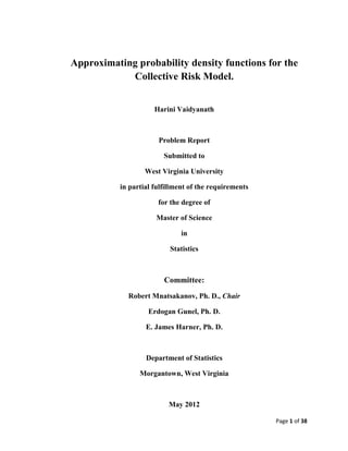
6.c
Graphical comparison of solutions from Panjer Recursion, Normal
approximation and Translated Gamma Approximation.

of 38
6.c
Interpretation of Graph:
It is seen that the normal approximation performs poorly and does a very bad job of
approximating right tail probabilities. The translated gamma approximation produces unstable
results because of the small values for the scale and shape parameter in the problem under
consideration.
7
Discussion and Conclusion:
The recursion techniques presented in this report are exact methods of calculating mass and
distribution functions of random claim size variables.
An important observation from the results in this report is that aggregate claim distributions are
almost always positively skewed which, as mentioned earlier, would be of interest to an
insurance company that is profit oriented.
One of the drawbacks of these techniques is that they are applicable only to the cases where the
claim random variables are distributed on non-negative integers, i.e. to discrete random
variables. In practice, the Pareto or lognormal distributions are often used to model individual
claim amounts. This poses a problem in using the recursion techniques as these distributions are
continuous. To overcome this situation, discretization methods can be used to replace continuous
distributions with appropriate discrete distributions distributed on non – negative integers. But
the distributions so obtained would be only approximate as information may be lost in the
discretization process.
For situations where intensive computing power poses a constraint, the normal approximation or
the translated approximation methods can be useful to the analyst to obtain the distribution
function of ‘g’ quickly. It is important to note that the translated gamma approximation
outperforms the normal approximation, especially when approximating right tail probabilities.
This is seen in the example using the Panjer Recursion Formula.
Another drawback is that recursion methods for computing mass functions in Schröter’s class are
lengthier than those from the (a,b,0) or (a,b,1) class because of the extra step required to
compute the probability functions of convolutions from the individual claim probability
functions.
Also, since claim causes are ignored, the results are only probabilistic in nature and not
inferential. If causes are taken into account, the IID assumption may not always be met. This

of 38
may be overcome by using modern statistical techniques like Multivariate analysis, Regression
Modeling, Data mining, etc to look at claims from an applied statistical point of view.
The results from such techniques would be advantageous to insurance companies as it would
help them study risks in more detail and decide how best to insure them. An example of such a
situation would be a decision making process on what kind of insurance coverage to provide to a
coal miner vs. a doctor.
An advantage of taking claim causes into consideration would be that in addition to modeling
techniques, predictive techniques can be introduced to predict future events, which would also be
very useful to insurance companies.
The topic of this report uses the term density function although the cases studied under recursion
are all discrete. This is because it is possible to study mass functions as a specialized case of
density functions, when the random variables are discrete, i.e. when it is possible to calculate
Pr(Xi = x).
8
References:
Text Books:
David C. M. Dickson (January, 2005), Insurance, Risk, and Ruin, CAMBRIDGE
Papers referred to for R code:
Paul Embrechts, Marco Frei, (July, 2010), PANJER RECURSION VS FFT FOR COMPOUND
DISTRIBUTIONS
Papers referred to for general definitions:
Bertil Almer (1967)

of 38
9
R codes:
Panjer Recursion Technique:
f <- vector(length = 30)
g <- vector(length = 31)
g[1] <- exp(-2)
for ( j in 1:30)
{
f[j] <- 0.6*((0.4)^(j-1))
for(x in j:30)
{
g[x+1] <- (2/x)*sum((1:j)*f[1:j]*g[x+1-(1:j)])
}
}
a <- c(1: 30)
a1 <- c(1: 31)
plot(a,f , type = "h", xlab = "Support of 'f' ", ylab = "Mass function 'f' ", main = "Individual
claim mass function 'f'", col = "green")
plot(a1,g, type = "h", xlab = "Support of 'g' ", ylab = "Mass function 'g' ", main = "Aggregate
claims mass function 'g'", col = "blue")
Extended Panjer Recursion Technique:
a <- 0.5
b <- -0.5
theta <- 0.5
f <- vector(length = 100)
q1 <- (-1/log(theta))*(theta)
f[1] <- 0.2
g[1]<- (log(1-(theta*f[1])) / log(1-theta))

of 38
for(j in 2:100)
{
f[j] <- 0.2 * (0.8 ^ (j-1))
for(x in 2:100)
{
g[x] <- (1/(1-(a*f[1])))*(sum((a+(b*j/x))*f[j]*g[x+1-j])+(q1*f[x]))
}
}
plot(1:100, f[1:100], type = "h", col = "green", main = "Individual claim mass function 'f'", xlab
= "Support of 'f'", ylab = "Mass function 'f'")
plot(1:100, g[1:100], type = "h", col = "blue", main = "Aggregate claims mass function 'g'", xlab
= "Support of 'g'", ylab = "Mass function'g'" )
Schröter’s class:
a <- 0.5
b <- 2.5
c <- -1
f <- c(0.4,0.35,0.25)
f_j <-c(0,0,0.16,0.28)
g[1] <- 0.25*exp(-2)
for(i in 2:4)
{
for(j in 2:i)
{
g[i] <- (1/(1-(a*f[1])))*sum((((a+(b*(j-1)/(i-1)))*f[j])+(((c*(j-1))/(2*(i-1)))*f_j[j]))*g[i+1-j])
}
}
plot(1:3, f, type = "h", col = "green", main = "Individual claims mass function 'f'", xlab =
"Support of 'f'", ylab = "Mass function 'f'")
plot(1:4, f_j, type = "h", col = "red", main = "Claim convolutions mass function 'f2*'", xlab =
"Support of 'f2*'", ylab = "Mass function 'f2*'")
plot(1:4, g[1:4], type = "h", col = "blue", main = "Aggregate claims mass function ", xlab =
"Support of 'g'", ylab = "Density function 'g'")

of 38
Comparison of results from Panjer Recursion, Normal
Approximation and Translated Gamma approximation:
q1 <- quantile(rnorm(50, mean = 3.3334, sd = sqrt(5.777774)), probs = seq(0, 1, 0.033))
q2 <- quantile(rgamma(50, shape = 0.002282604, rate = 0.01987627), probs = seq(0, 1, 0.033))
ngpv <- c(1:31)
ngp <- dnorm(q1, mean = 3.3334, sd = sqrt(5.777774))
tgpv <- c(1:31)
k<- 3.218559
tgpv1 <- tgpv - k
tgp <- dgamma(q2, shape = 0.002282604, rate = 0.01987627)
par(mfrow = c(3,1))
plot(a1,g, type = "h", xlab = "Support of ' g '", ylab = "Probability mass function ' g '", main = "'
g ' obtained using Panjer Recursion Technique ", col = "blue")
plot(ngpv, ngp, type = "l", xlab = "Support of 'g'", ylab = "Probability density function ' g '",
main = "' g ' obtained using Normal Approximation", col = "orange")
plot(tgpv1, tgp, type = "l", xlab = "Support of 'g'", ylab = "Probability density function 'g'", main
= "' g ' obtained using Translated Gamma Approximation", col = "green", xlim = c(0,30))

Approximating_probability_density_functions_for_the_Collective_Risk_Model

Recommended

Recommended

More Related Content

What's hot

What's hot (6)

Viewers also liked

Viewers also liked (14)

Similar to Approximating_probability_density_functions_for_the_Collective_Risk_Model

Similar to Approximating_probability_density_functions_for_the_Collective_Risk_Model (20)

Approximating_probability_density_functions_for_the_Collective_Risk_Model