This document provides an excerpt from the book "Spark: The Definitive Guide" which introduces some of the core concepts of Apache Spark. It discusses Spark's basic architecture including the driver program, executors, and cluster managers. It also covers Spark applications, DataFrames, transformations and actions. Finally, it provides a sample end-to-end example reading CSV flight data to demonstrate these concepts.

1. 1
Spark
The Definitive Guide
Excerpts from the upcoming book on making
big data simple with Apache Spark.
By Bill Chambers & Matei Zaharia

2. Apache Spark has seen immense growth over the past
several years. The size and scale of Spark Summit 2017 is
a true reflection of innovation after innovation that has
made itself into the Apache Spark project. Databricks
is proud to share excerpts from the upcoming book,
Spark: The Definitive Guide. Enjoy this free preview copy,
courtesy of Databricks, of chapters 2, 3, 4, and 5 and
subscribe to the Databricks blog for upcoming chapter
releases.
Preface
2

3. A Gentle Introduction to Spark
This chapter will present a gentle introduction to Spark. We will walk through the core architecture of a cluster, Spark
Application, and Spark’s Structured APIs using DataFrames and SQL. Along the way we will touch on Spark’s core
terminology and concepts so that you are empowered start using Spark right away. Let’s get started with some basic
background terminology and concepts.
Spark’s Basic Architecture
Typically when you think of a “computer” you think about one machine sitting on your desk at home or at work. This
machine works perfectly well for watching movies or working with spreadsheet software. However, as many users
likely experience at some point, there are some things that your computer is not powerful enough to perform. One
particularly challenging area is data processing. Single machines do not have enough power and resources to perform
computations on huge amounts of information (or the user may not have time to wait for the computation to finish).
A cluster, or group of machines, pools the resources of many machines together allowing us to use all the cumulative
resources as if they were one. Now a group of machines alone is not powerful, you need a framework to coordinate
work across them. Spark is a tool for just that, managing and coordinating the execution of tasks on data across a
cluster of computers.
The cluster of machines that Spark will leverage to execute tasks will be managed by a cluster manager like Spark’s
Standalone cluster manager, YARN, or Mesos. We then submit Spark Applications to these cluster managers which will
grant resources to our application so that we can complete our work.
Spark Applications
Spark Applications consist of a driver process and a set of executor processes. The driver process, Figure 1-2, sits
on a node in the cluster and is responsible for three things: maintaining information about the Spark application;
responding to a user’s program; and analyzing, distributing, and scheduling work across the executors. As suggested
by the following figure, the driver process is absolutely essential - it’s the heart of a Spark Application and maintains
all relevant information during the lifetime of the application.
3

4. The driver maintains the work to be done, the executors are responsible for only two things: executing code assigned
to it by the driver and reporting the state of the computation, on that executor, back to the driver node.
The last piece relevant piece for us is the cluster manager. The cluster manager controls physical machines and
allocates resources to Spark applications. This can be one of several core cluster managers: Spark’s standalone
cluster manager, YARN, or Mesos. This means that there can be multiple Spark applications running on a cluster at
the same time. We will talk more in depth about cluster managers in Part IV: Production Applications of this book. In
the previous illustration we see on the left, our driver and on the right the four executors on the right. In this diagram,
we removed the concept of cluster nodes. The user can specify how many executors should fall on each node through
configurations.
note
Spark, in addition to its cluster mode, also has a local mode. The driver and executors are simply processes, this
means that they can live on a single machine or multiple machines. In local mode, these run (as threads) on your
individual computer instead of a cluster. We wrote this book with local mode in mind, so everything should be
runnable on a single machine.
As a short review of Spark Applications, the key points to understand at this point are that:
• Spark has some cluster manager that maintains an understanding of the resources available.
• The driver process is responsible for executing our driver program’s commands accross the executors in order to
complete our task.
Now while our executors, for the most part, will always be running Spark code. Our driver can be “driven” from a
number of different languages through Spark’s Language APIs.
Figure
JVM
User Code
To Executors
Spark Session
Spark Application
4

5. Figure 2:
Driver Process Executors
User Code
Spark Session
Cluster Manager
Spark’s Language APIs
Spark’s language APIs allow you to run Spark code from other langauges. For the most part, Spark presents some core
“concepts” in every language and these concepts are translated into Spark code that runs on the cluster of machines.
If you use the Structured APIs (Part II of this book), you can expect all languages to have the same performance
characteristics.
note
This is a bit more nuanced than we are letting on at this point but for now, it’s true “enough”. We cover this
extensively in first chapters of Part II of this book.
5

6. Scala
Spark is primarily written in Scala, making it Spark’s “default” language. This book will include Scala code examples
wherever relevant.
Python
Python supports nearly all constructs that Scala supports. This book will include Python code examples whenever we
include Scala code examples and a Python API exists.
SQL
Spark supports ANSI SQL 2003 standard. This makes it easy for analysts and non-programmers to leverage the big
data powers of Spark. This book will include SQL code examples wherever relevant
Java
Even though Spark is written in Scala, Spark’s authors have been careful to ensure that you can write Spark code in
Java. This book will focus primarily on Scala but will provide Java examples where relevant.
R
Spark has two libraries, one as a part of Spark core (SparkR) and another as a R community driven package (sparklyr).
We will cover these two different integrations in Part VII: Ecosystem.
6

7. Here’s a simple illustration of this relationship.
Each language API will maintain the same core concepts that we described above. There is a SparkSession available
to the user, the SparkSession will be the entrance point to running Spark code. When using Spark from a Python or
R, the user never writes explicit JVM instructions, but instead writes Python and R code that Spark will translate into
code that Spark can then run on the executor JVMs. There is plenty more detail about this implementation that we
cover in later parts of the book but for the most part the above section should be plenty for you to use and leverage
Spark successfully.
Starting Spark
Thus far we covered the basics concepts of Spark Applications. At this point it’s time to dive into Spark itself and
understand how we actually go about leveraging Spark. To do this we will start Spark’s local mode, just like we did
in the previous chapter, this means running ./bin/spark-shell to access the Scala console. You can also start
Python console with ./bin/pyspark. This starts an interactive Spark Application. There is another method for
submitting applications to Spark called spark-submit which does not allow for a user console but instead executes
prepared user code on the cluster as its own application. We discuss spark-submit in Part IV of the book. When we
start Spark in this interactive mode, we implicitly create a SparkSession which manages the Spark Application.
SparkSession
As discussed in the beginning of this chapter, we control our Spark Application through a driver process. This driver
process manifests itself to the user as something called the SparkSession. The SparkSession instance is the way Spark
exeutes user-defined manipulations across the cluster. In Scala and Python the variable is available as spark when
you start up the console. Let’s go ahead and look at the SparkSession in both Scala and/or Python.
Figure
Spark Session User Code
JVM Python/R Process
7

8. spark
In Scala, you should see something like:
res0: org.apache.spark.sql.SparkSession = org.apache.spark.sql.SparkSession@27159a24
In Python you’ll see something like:
<pyspark.sql.session.SparkSession at 0x7efda4c1ccd0>
Let’s now perform the simple task of creating a range of numbers. This range of numbers is just like a named column
in a spreadsheet.
%scala
val myRange = spark.range(1000).toDF(“number”)
%python
myRange = spark.range(1000).toDF(“number”)
You just ran your first Spark code! We created a DataFrame with one column containing 1000 rows with values from
0 to 999. This range of number represents a distributed collection. When run on a cluster, each part of this range of
numbers exists on a different executor. This range is what Spark defines as a DataFrame.
DataFrames
A DataFrame is a table of data with rows and columns. The list of columns and the types in those columns is the
schema. A simple analogy would be a spreadsheet with named columns. The fundamental difference is that while a
spreadsheet sits on one computer in one specific location, a Spark DataFrame can span thousands of computers. The
reason for putting the data on more than one computer should be intuitive: either the data is too large to fit on one
machine or it would simply take too long to perform that computation on one machine. The DataFrame concept is not
unique to Spark. R and Python both have similar concepts. However, Python/R DataFrames (with some exceptions)
exist on one machine rather than multiple machines. This limits what you can do with a given DataFrame in python
and R to the resources that exist on that specific machine. However, since Spark has language interfaces for both
Python and R, it’s quite easy to convert to Pandas (Python) DataFrames
8

9. note
Spark has several core abstractions: Datasets, DataFrames, SQL Tables, and Resilient Distributed Datasets
(RDDs). These abstractions all represent distributed collections of data however they have different interfaces
for working with that data. The easiest and most efficient are DataFrames, which are available in all languages.
We cover Datasets at the end of Part II and RDDs in Part III of this book. The following concepts apply to all of the
core abstractions.
Partitions
In order to allow every executor to perform work in parallel, Spark breaks up the data into chunks, called partitions. A
partition is a collection of rows that sit on one physical machine in our cluster. A DataFrame’s partitions represent how
the data is physically distributed across your cluster of machines during execution. If you have one partition, Spark
will only have a parallelism of one even if you have thousands of executors. If you have many partitions, but only one
executor Spark will still only have a parallelism of one because there is only one computation resource.
An important thing to note, is that with DataFrames, we do not (for the most part) manipulate partitions individually.
We simply specify high level transformations of data in the physical partitions and Spark determines how this work
will actually execute on the cluster. Lower level APIs do exist (via the RDD interface) and we cover those in Part III of
this book.
Transformations
In Spark, the core data structures are immutable meaning they cannot be changed once created. This might seem like
a strange concept at first, if you cannot change it, how are you supposed to use it? In order to “change” a DataFrame
you will have to instruct Spark how you would like to modify the DataFrame you have into the one that you want.
These instructions are called transformations.
Figure
Table or DataFrame partitioned
across servers in data center
Spreadsheet on a
single machine
9

10. Let’s perform a simple transformation to find all even numbers in our currentDataFrame.
%scala
val divisBy2 = myRange.where(“number % 2 = 0”)
%python
divisBy2 = myRange.where(“number % 2 = 0”)
You will notice that these return no output, that’s because we only specified an abstract transformation and Spark
will not act on transformations until we call an action, discussed shortly. Transformations are the core of how you
will be expressing your business logic using Spark. There are two types of transformations, those that specify narrow
dependencies and those that specify wide dependencies. Transformations consisting of narrow dependencies
are those where each input partition will contribute to only one output partition. Our where clause specifies a
narrow dependency, where only one partition contributes to at most one output partition. A wide dependency style
transformation will have input partitions contributing to many output partitions. We call this a shuffle where Spark
will exchange partitions across the cluster. Spark will automatically perform an operation called pipelining on narrow
dependencies, this means that if we specify multiple filters on DataFrames they’ll all be performed in memory. The
same cannot be said for shuffles. When we perform a shuffle, Spark will write the results to disk. You’ll see lots of talks
about shuffle optimization across the web because it’s an important topic but for now all you need to understand are
that there are two kinds of transformations.
This brings ups our next concept, transformations are abstract manipulations of data that Spark will execute lazily.
Lazy Evaluation
Lazy evaulation means that Spark will wait until the very last moment to execute your transformations. In Spark,
instead of modifying the data quickly, we build up a plan of transformations that we would like to apply to our source
data. Spark, by waiting until the last minute to execute the code, will compile this plan from your raw, DataFrame
transformations, to an efficient physical plan that will run as efficiently as possible across the cluster. This provides
immense benefits to the end user because Spark can optimize the entire data flow from end to end. An example of this
might be “predicate pushdown”. If we build a large Spark job consisting of narrow dependencies, but specify a filter at
the end that only requires us to fetch one row from our source data, the most efficient way to execute this is to access
the single record that we need. Spark will actually optimize this for us by pushing the filter down automatically.
10

11. Actions
Transformations allow us to build up our logical transformation plan. To trigger the computation, we run an action. An
action instructs Spark to compute a result from a series of transformations. The simplest action is count which gives
us the total number of records in the DataFrame.
divisBy2.count()
We now see a result! There are 500 number divisible by two from o to 999 (big surprise!). Now count is not the only
action. There are three kinds of actions:
• actions to view data in the console;
• actions to collect data to native objects in the respective language;
• and actions to write to output data sources.
In specifying our action, we started a Spark job that runs our filter transformation (a narrow transformation), then an
aggregation (a wide transformation) that performs the counts on a per partition basis, then a collect will brings our
result to a native object in the respective language. We can see all of this by inspecting the Spark UI, a tool included in
Spark that allows us to monitor the Spark jobs running on a cluster.
Spark UI
During Spark’s execution of the previous code block, users can monitor the progress of their job through the Spark UI.
The Spark UI is available on port 4040 of the driver node. If you are running in local mode this will just be the
http://localhost:4040. The Spark UI maintains information on the state of our Spark jobs, environment, and
cluster state. It’s very useful, especially for tuning and debugging. In this case, we can see one Spark job with two
stages and nine tasks were executed.
This chapter avoids the details of Spark jobs and the Spark UI. At this point you should understand that a Spark job
represents a set of transformations triggered by an individual action and we can monitor that from the Spark UI. We
do cover the Spark UI in detail in Part IV: Production Applications of this book.
11

12. Figure 5
An End to End Example
In the previous example, we created a DataFrame of a range of numbers. Not exactly groundbreaking big data. In
this section we will reinforce everything we learned previously in this chapter with a worked example and explaining
step by step what is happening under the hood. We’ll be using some flight data available here from the United States
Bureau of Transportation statistics.
Inside of the CSV folder linked above, you’ll see that we have a number of files. You will also notice a number of other
folders with different file formats that we will discuss in Part II: Reading and Writing data.
%fs ls /mnt/defg/flight-data/csv/
Each file has a number of rows inside of it. Now these files are CSV files, meaning that they’re a semi-structured data
format with a row in the file representing a row in our future DataFrame.
$ head /mnt/defg/flight-data/csv/2015-summary.csv
DEST_COUNTRY_NAME,ORIGIN_COUNTRY_NAME,count
United States,Romania,15
United States,Croatia,1
United States,Ireland,344
12

13. Spark includes the ability to read and write from a large number of data sources. In order to read this data in, we will
use a DataFrameReader that is associated with our SparkSession. In doing so, we will specify the file format as well as
any options we want to specify. In our case, we want to do something called schema inference, we want Spark to take
a best guess at what the schema of our DataFrame should be. The reason for this is that CSV files are not completely
structured data formats. We also want to specify that the first row is the header in the file, we’ll specify that as an
option too.
To get this information Spark will read in a little bit of the data and then attempt to parse the types in those rows
according to the types available in Spark. You’ll see that it does a good job. We also have the option of strictly
specifying a schema when we read in data.
%scala
val flightData2015 = spark
.read
.option(“inferSchema”, “true”)
.option(“header”, “true”)
.csv(“/mnt/defg/flight-data/csv/2015-summary.csv”)
%python
flightData2015 = spark
.read
.option(“inferSchema”, “true”)
.option(“header”, “true”)
.csv(“/mnt/defg/flight-data/csv/2015-summary.csv”)
Each of these DataFrames (in Scala and Python) each have a set of columns with an unspecified number of rows.
The reason the number of rows is “unspecified” is because reading data is a transformation, and is therefore a lazy
operation. Spark only peeked at the data to try to guess what types each column should be.
Figure
JSON
file
flightData2015
DataFrame
read
Lazy Eager
take (2)
Array( Row(...),Row(...))
13

14. If we perform the take action on the DataFrame, we will be able to see the same results that we saw before when we
used the command line.
flightData2015.take(3)
Let’s specify some more transformations! Now we will sort our data according to the count column which is an
integer type.
note
Remember, the sort does not modify the DataFrame. We use the sort is a transformation that returns a new
DataFrame by transforming the previous DataFrame. Let’s take a look at this transformation as an illustration.
Nothing will happen to the data when we call this sort because it’s just a transformation. However, we can see that
Spark is building up a plan for how it will execute this across the cluster by looking at the explain plan. We can call
explain on any DataFrame object to see the DataFrame’s lineage.
flightData2015.sort(“count”).explain()
Congratulations, you’ve just read your first explain plan! Explain plans are a bit arcane, but with a bit of practice it
becomes second nature. Explain plans can be read from top to bottom, the top being the end result and the bottom
Figure 7:
JSON file
Read
DataFrame
Sort
DataFrame
14

15. being the source(s) of data. In our case, just take a look at the first keywords. You will see “sort”, “exchange”, and
“FileScan”. That’s because the sort of our data is actually a wide dependency because rows will have to be compared
with one another. Don’t worry too much about understanding everything about explain plans, they can just be helpful
tools for debugging and improving your knowledge as you progress with Spark.
Now, just like we did before, we can specify an action in order to kick off this plan.
flightData2015.sort(“count”).take(2)
This will get us the sorted results, as expected. This operation is illustrated in the following image.
The logical plan of transformations that we build up defines a lineage for the DataFrame so that at any given point in
time Spark knows how to recompute any partition by performing all of the operations it had before on the same input
data. This sits at the heart of Spark’s programming model, functional programming where the same inputs always
result in the same outputs when the transformations on that data stay constant.
Now that we performed this action, remember that we can navigate to the Spark UI (port 4040) and see the
information about this jobs stages and tasks.
DataFrames and SQL
We worked through a simple example in the previous example, let’s now work through a more complex example and
follow along in both DataFrames and SQL. For your purposes, DataFrames and SQL, in Spark, are the exact same
thing. You can express your business logic in either language and Spark will compile that logic down to an underlying
plan (that we see in the explain plan) before actually executing your code. Spark SQL allows you as a user to register
any DataFrame as a table or view (a temporary table) and query it using pure SQL. There is no performance difference
between writing SQL queries or writing DataFrame code, they both “compile” to the same underlying plan that we
specify in DataFrame code.
Figure
JSON file
Read
DataFrame
Sort take(2)
DataFrame
Array(...)
15

16. Any DataFrame can be made into a table or view with one simple method call.
%scala
flightData2015.createOrReplaceTempView(“flight_data_2015”)
%python
flightData2015.createOrReplaceTempView(“flight_data_2015”)
Now we can query our data in SQL. To execute a SQL query, we’ll use the spark.sql function (remember spark is
our SparkSession variable?) that conveniently, returns a new DataFrame. While this may seem a bit circular in logic
- that a SQL query against a DataFrame returns another DataFrame, it’s actually quite powerful. As a user, you can
specify transformations in the manner most convenient to you at any given point in time and not have to trade any
efficiency to do so! To understand that this is happening, let’s take a look at two explain plans.
%scala
val sqlWay = spark.sql(“””
SELECT DEST_COUNTRY_NAME, count(1)
FROM flight_data_2015
GROUP BY DEST_COUNTRY_NAME
“””)
val dataFrameWay = flightData2015
.groupBy(‘DEST_COUNTRY_NAME)
.count()
sqlWay.explain
dataFrameWay.explain
%python
sqlWay = spark.sql(“””
SELECT DEST_COUNTRY_NAME, count(1)
FROM flight_data_2015
GROUP BY DEST_COUNTRY_NAME
“””)
16

17. dataFrameWay = flightData2015
.groupBy(“DEST_COUNTRY_NAME”)
.count()
sqlWay.explain()
dataFrameWay.explain()
We can see that these plans compile to the exact same underlying plan!
To reinforce the tools available to us, let’s pull out some interesting statistics from our data. One thing to understand
is that DataFrames (and SQL) in Spark already have a huge number of manipulations available. There are hundreds
of functions that you can leverage and import to help you resolve your big data problems faster. We will use the max
function, to find out what the maximum number of flights to and from any given location are. This just scans each
value in relevant column the DataFrame and sees if it’s bigger than the previous values that have been seen. This is a
transformation, as we are effectively filtering down to one row. Let’s see what that looks like.
// scala or python
spark.sql(“SELECT max(count) from flight_data_2015”).take(1)
%scala
import org.apache.spark.sql.functions.max
flightData2015.select(max(“count”)).take(1)
%python
from pyspark.sql.functions import max
flightData2015.select(max(“count”)).take(1)
Great, that’s a simple example. Let’s perform something a bit more complicated and find out the top five destination
countries in the data set? This is a our first multi-transformation query so we’ll take it step by step. We will start with a
fairly straightforward SQL aggregation.
17

18. %scala
val maxSql = spark.sql(“””
SELECT DEST_COUNTRY_NAME, sum(count) as destination_total
FROM flight_data_2015
GROUP BY DEST_COUNTRY_NAME
ORDER BY sum(count) DESC
LIMIT 5
“””)
maxSql.collect()
%python
maxSql = spark.sql(“””
SELECT DEST_COUNTRY_NAME, sum(count) as destination_total
FROM flight_data_2015
GROUP BY DEST_COUNTRY_NAME
ORDER BY sum(count) DESC
LIMIT 5
“””)
maxSql.collect()
Now let’s move to the DataFrame syntax that is semantically similar but slightly different in implementation and
ordering. But, as we mentioned, the underlying plans for both of them are the same. Let’s execute the queries and see
their results as a sanity check.
%scala
import org.apache.spark.sql.functions.desc
flightData2015
.groupBy(“DEST_COUNTRY_NAME”)
.sum(“count”)
.withColumnRenamed(“sum(count)”, “destination_total”)
.sort(desc(“destination_total”))
.limit(5)
.collect()
18

19. %python
from pyspark.sql.functions import desc
flightData2015
.groupBy(“DEST_COUNTRY_NAME”)
.sum(“count”)
.withColumnRenamed(“sum(count)”, “destination_total”)
.sort(desc(“destination_total”))
.limit(5)
.collect()
Now there are 7 steps that take us all the way back to the source data. You can see this in the explain plan on those
DataFrames. Illustrated below are the set of steps that we perform in “code”. The true execution plan (the one visible
in explain) will differ from what we have below because of optimizations in physical execution, however the llustration
is as good of a starting point as any. This execution plan is a directed acyclic graph (DAG) of transformations, each
resulting in a new immutable DataFrame, on which we call an action to generate a result.
The first step is to read in the data. We defined the DataFrame previously but, as a reminder, Spark does not actually
read it in until an action is called on that DataFrame or one derived from the original DataFrame.
The second step is our grouping, technically when we call groupBy we end up with a RelationalGroupedDataset
which is a fancy name for a DataFrame that has a grouping specified but needs a user to specify an aggregation before
it can be queried further. We can see this by trying to perform an action on it (which will not work). We still haven’t
performed any computation (besides relational algebra) - we’re simply passing along information about the layout of
Figure 9:
CSV file
Read
DataFrame DataFrame
DataFrame
groupBy
Sort
DataFrame
Collect Limit
Grouped Dataset
DataFrame
Array(...)
Our result
Column
renamed
19

20. the data.
Therefore the third step is to specify the aggregation. Let’s use the sum aggregation method. This takes as input
a column expression or simply, a column name. The result of the sum method call is a new dataFrame. You’ll see
that it has a new schema but that it does know the type of each column. It’s important to reinforce (again!) that no
computation has been performed. This is simply another transformation that we’ve expressed and Spark is simply
able to trace the type information we have supplied.
The fourth step is a simple renaming, we use the withColumnRenamed method that takes two arguments, the
original column name and the new column name. Of course, this doesn’t perform computation - this is just another
transformation!
The fifth step sorts the data such that if we were to take results off of the top of the DataFrame, they would be the
largest values found in the destination_total column.
You likely noticed that we had to import a function to do this, the desc function. You might also notice that desc
does not return a string but a Column. In general, many DataFrame methods will accept Strings (as column names) or
Column types or expressions. Columns and expressions are actually the exact same thing.
The final step is just a limit. This just specifies that we only want five values. This is just like a filter except that it filters
by position (lazily) instead of by value. It’s safe to say that it basically just specifies a DataFrame of a certain size.
The last step is our action! Now we actually begin the process of collecting the results of our DataFrame above and
Spark will give us back a list or array in the language that we’re executing. Now to reinforce all of this, let’s look at the
explain plan for the above query.
%scala
flightData2015
.groupBy(“DEST_COUNTRY_NAME”)
.sum(“count”)
.withColumnRenamed(“sum(count)”, “destination_total”)
.sort(desc(“destination_total”))
.limit(5)
.explain()
%python
flightData2015
.groupBy(“DEST_COUNTRY_NAME”)
.sum(“count”)
.withColumnRenamed(“sum(count)”, “destination_total”)
20

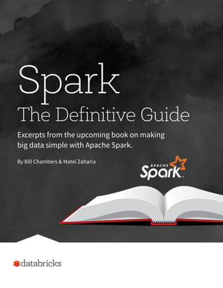
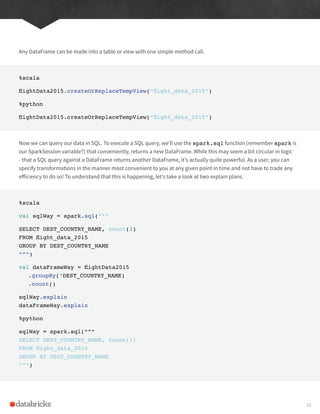
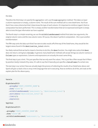
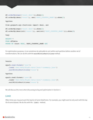
21. .sort(desc(“destination_total”))
.limit(5)
.explain()
== Physical Plan ==
TakeOrderedAndProject(limit=5, orderBy=[destination_total#16194L DESC],
output=[DEST_COUNTRY_
+- *HashAggregate(keys=[DEST_COUNTRY_NAME#7323], functions=[sum(count#7325L)])
+- Exchange hashpartitioning(DEST_COUNTRY_NAME#7323, 5)
+- *HashAggregate(keys=[DEST_COUNTRY_NAME#7323], functions=[partial_
sum(count#7325L)])
+- InMemoryTableScan [DEST_COUNTRY_NAME#7323, count#7325L]
+- InMemoryRelation [DEST_COUNTRY_NAME#7323, ORIGIN_COUNTRY_NAME#7324, count#
+- *Scan csv [DEST_COUNTRY_NAME#7578,ORIGIN_COUNTRY_NAME#7579,count#7580L]
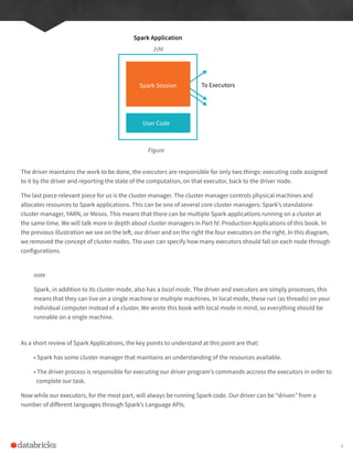
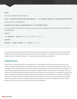
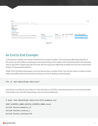
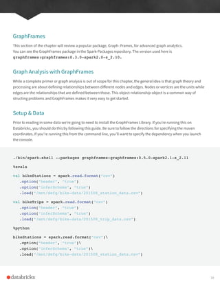
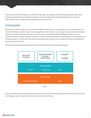
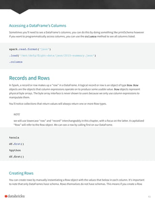
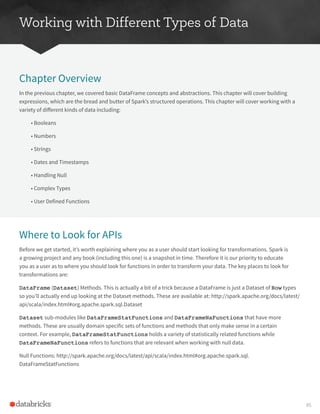
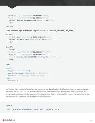
While this explain plan doesn’t match our exact “conceptual plan” all of the pieces are there. You can see the limit
statement as well as the orderBy (in the first line). You can also see how our aggregation happens in two phases, in
the partial_sum calls. This is because summing a list of numbers is commutative and Spark can perform the sum,
partition by partition. Of course we can see how we read in the DataFrame as well.
Naturally, we don’t always have to collect the data. We can also write it out to any data source that Spark supports.
For instance, let’s say that we wanted to store the information in a database, we could write these results out to JDBC.
We could also write them out to a new file.
This chapter introduces the basics of Spark. We talked about transformations and actions, how Spark lazily executes
a DAG of transformations in order to optimize the execution plan on DataFrames. We talked about how data is
organized into partitions and set the stage for working with more complex transformations. The next chapter will help
show you around the vast Spark ecosystem. We will see some more advanced concepts and tools that are available
in Spark, from Streaming to Machine Learning, to explore all that Spark has to offer in addition to the features and
concepts covered in this chapter.
21

22. A Tour of Spark’s Toolset
In the previous chapter we introduced Spark’s core concepts like transformations and actions. These simple
conceptual building blocks have created an entire ecosystem of tools that leverage Spark for a variety of different
tasks, from graph analysis and machine learning to streaming and integrations. These conceptual building blocks
are the tools that you will use throughout your time with Spark and allow you to understand how Spark executes
your workloads.
Let’s take a look at the following illustration of Spark’s functionality.
In the first chapter, we covered most of Spark’s Structured APIs, especially DataFrames and SQL. This chapter will
touch on all the other pieces of functionality in Spark’s toolset. It should come as no surprise that this diagram
effectively mirrors the individual parts of the book except that we start at the heart with DataFrames and SQL and
then work our way out to the different higher level building blocks.
This chapter will aim to share a number of things that you can do with Spark at a higher level.
We’ll start by covering a bit more about Spark’s core functionality and touch on the lower level APIs. We will then
cover Structured Streaming before performing some advanced analytics and looking at Spark’s package ecosystem.
The entire book covers these topics in depth, the goal of this chapter is simply the tour. Allowing you as a user to
“choose your own adventure” and dive into what interests you most next.
Figure
Structured APIs
DataFrames SQL
Datasets
Structured
streaming
Advanced analytics
ML graph
Deep learning
Ecosystem
+
Packages
Low level APIs
Distributed variables RDDs
22

23. Datasets
If you followed the development of Spark in the past year, you will undoubtedly heard of Datasets. DataFrames are
a distributed collection of objects of type Row (more in the next chapter) but Spark also allows JVM users to create
their own objects (via case classes or java beans) and manipulate them using function programming concepts. For
instance, rather than creating a range and manipulating it via SQL or DataFrames, we can manipulate it just as we
might manipulate a local scala collection. We can map over the values with a user defined function, and convert it into
a new arbitrary case class object.
The amazing thing about Datasets is that we can use them only when we need or want to. For instance, in the
following example I’ll define my own object and manipulate it via arbitrary map and filter functions. Once we’ve
performed our manipulations, Spark can automatically turn it back into a DataFrame and we can manipulate it
further using the hundreds of functions that Spark includes. This makes it easy to drop down to lower level, type
secure coding when necessary, and move higher up to SQL for more rapid analysis. We cover this material extensively
in the next part of this book, but this ability to manipulate arbitrary case classes with arbitrary functions makes
expressing business logic simple.
case class ValueAndDouble(value:Long, valueDoubled:Long)
spark.range(2000)
.map(value => ValueAndDouble(value, value * 2))
.filter(vAndD => vAndD.valueDoubled % 2 == 0)
.where(“value % 3 = 0”)
.count()
Caching Data for Faster Access
We discussed wide and narrow transformations in the previous chapter and how Spark automatically spills to disk
when we perform a shuffle. However, sometimes we’re going to access a DataFrame multiple times in the same data
flow and we want to avoid performing expensive joins over and over again. Imagine that we were to access the initial
data set numerous times. A smart thing to do would be to cache the data in memory since we repeatedly access this
data. Now remember that a DataFrame always has to go back to a robust data source as its origin, caching is simply a
23

24. way to create a new “origin” along the way. Let’s illustrate this with a drawing.
You’ll see here that we have our “lazily” created DataFrame along with the DataFrames that we will create in the
future. The problem is that all of our downstream DataFrames share a common parent and they all have to do the
work of creating that same DataFrame. In this case it’s just reading in the raw data but that can be a fairly intensive
process - especially for large datasets. Let’s just perform this exact example and see how long it takes.
%scala
val DF1 = spark.read.format(“csv”)
.option(“inferSchema”, “true”)
.option(“header”, “true”)
.load(“/mnt/defg/flight-data/csv/2015-summary.csv”)
%python
DF1 = spark.read.format(“csv”)
.option(“inferSchema”, “true”)
.option(“header”, “true”)
.load(“/mnt/defg/flight-data/csv/2015-summary.csv”)
Figure 2:
2015-summary.csv
Initial DataFrame
Group by
destination
DF2 DF3 DF4 DFS
Group by
origin
Group by
count Sum(count)
24

25. %scala
val DF2 = DF1.groupBy(“DEST_COUNTRY_NAME”).count().collect()
val DF3 = DF1.groupBy(“ORIGIN_COUNTRY_NAME”).count().collect()
val df4 = DF1.groupBy(“count”).count().collect()
%python
DF2 = DF1.groupBy(“DEST_COUNTRY_NAME”).count().collect()
DF3 = DF1.groupBy(“ORIGIN_COUNTRY_NAME”).count().collect()
DF4 = DF1.groupBy(“count”).count().collect()
Now on my machine that took about 2.75 seconds. Luckily caching can help speed things up. When we specify a
DataFrame to be cached, the first time that Spark reads it in - it will save it to be accessed again later. Then when any
other queries come along, they’ll just refer to the one stored in memory as opposed to the original file.
Rather than having to recompute that initial DataFrame we can save it into memory with the cache method. This will
cut down on the rest of the computation because Spark will already have the data stored in memory.
%scala
DF1.cache()
DF1.count()
%python
DF1.cache()
Figure 3:
Raw data
DF1
DF1
Cache
25

26. DF1.count()
%scala
val DF2 = DF1.groupBy(“DEST_COUNTRY_NAME”).count().collect()
val DF3 = DF1.groupBy(“ORIGIN_COUNTRY_NAME”).count().collect()
val df4 = DF1.groupBy(“count”).count().collect()
%python
DF2 = DF1.groupBy(“DEST_COUNTRY_NAME”).count().collect()
DF3 = DF1.groupBy(“ORIGIN_COUNTRY_NAME”).count().collect()
df4 = DF1.groupBy(“count”).count().collect()
We can see that this cuts the time by more than half! This may not seem that wild but picture a large data set or one
that requires a lot of computation in order to create (not just reading in a file). The savings can be immense. It’s also
great for iterative machine learning workloads because they’ll often have to access the same data a number of times
which we’ll see shortly.
Now sometimes our data may be too large to fit into memory. That’s why there’s also the persist method and
a number of options for us to save data to the disk of our machine. We discuss this in Part IV of the book when we
discuss optimizations and tuning.
Structured Streaming
Structured Streaming became Production Ready in Spark 2.2. Structured streaming allows you to take the same
operations that you perform in batch mode and perform them in a streaming fashion. This can reduce latency and
allow for incremental processing. The best thing about Structured Streaming is that it allows you to rapidly and
quickly get value out of streaming systems with simple switches, it also makes it easy to reason about because you
can write your batch job as a way to prototype it and then you can convert it to streaming job. The way all of this
works is by incrementally processing that data.
Let’s walk through a simple example of how easy it is to get started with Structured Streaming. For this we will use an
retail dataset. One that has specific dates and times for us to be able to use. When we list the directory, you will notice
that there are a variety of different files in there.
%fs ls /mnt/defg/retail-data/by-day/
The first thing that you’ll notice is that we’ve got a lot of different files. This is to process. Now this is retail data so
26

27. imagine that these are being produced by retail stores and sent to a location where they will be read by our Structured
Streaming job. Now in order to ground this, let’s first analyze the data as a static dataset and create a DataFrame to do
so. We’ll also create a schema so that when we read the data in later we don’t have to infer it.
%scala
val staticDataFrame = spark.read.format(“csv”)
.option(“header”, “true”)
.option(“inferSchema”, “true”)
.load(“dbfs:/mnt/defg/retail-data/by-day/*.csv”)
staticDataFrame.createOrReplaceTempView(“retail_data”)
val staticSchema = staticDataFrame.schema
%python
staticDataFrame = spark.read.format(“csv”)
.option(“header”, “true”)
.option(“inferSchema”, “true”)
.load(“dbfs:/mnt/defg/retail-data/by-day/*.csv”)
staticDataFrame.createOrReplaceTempView(“retail_data”)
staticSchema = staticDataFrame.schema
Now since we’re working with time series data it’s worth mentioning how we might go along grouping and
aggregating our data. In this example we’ll take a look at the largest sale hours where a given customer (identified by
CustomerId) makes a large purchase. For example, let’s add a total cost column and see on what days a customer
spent the most.
import org.apache.spark.sql.functions.{window, column, desc, col}
staticDataFrame
.selectExpr(
“CustomerId”,
“(UnitPrice * Quantity) as total_cost”,
“InvoiceDate”)
.groupBy(
27

28. col(“CustomerId”), window(col(“InvoiceDate”), “1 day”))
.sum(“total_cost”)
.orderBy(desc(“sum(total_cost)”))
.take(5)
%python
from pyspark.sql.functions import window, column, desc, col
staticDataFrame
.selectExpr(
“CustomerId”,
“(UnitPrice * Quantity) as total_cost” ,
“InvoiceDate” )
.groupBy(
col(“CustomerId”), window(col(“InvoiceDate”), “1 day”))
.sum(“total_cost”)
.orderBy(desc(“sum(total_cost)”))
.take(5)
%sql
SELECT
sum(total_cost),
CustomerId,
to_date(InvoiceDate)
FROM
(SELECT
CustomerId,
(UnitPrice * Quantity) as total_cost,
InvoiceDate
FROM
retail_data)
GROUP BY
CustomerId, to_date(InvoiceDate)
ORDER BY
sum(total_cost) DESC
That’s the static DataFrame version, there shouldn’t be any big surprises in there if you’re familiar with the syntax.
Now we’ve seen how that works, let’s take a look at the streaming code! You’ll notice that very little actually changes
about our code. The biggest change is that we used readStream instead of read, additionally you’ll notice
28

29. maxFilesPerTrigger option which simply specifies the number of files we should read in at once. This is to make
our demonstration more “streaming” and in a production scenario this would be omitted.
Now since you’re likely running this in local mode, it’s a good practice to set the number of shuffle partitions to
something that’s going to be a better fit for local mode. This configuration simple specifies the number of partitions
that should be created after a shuffle, by default the value is 200 but since there aren’t many executors on my local
machine it’s worth reducing this to five.
spark.conf.set(“spark.sql.shuffle.partitions”, “5”)
val streamingDataFrame = spark.readStream
.schema(staticSchema)
.option(“maxFilesPerTrigger”, 1)
.format(“csv”)
.option(“header”, “true”)
.load(“dbfs:/mnt/defg/retail-data/by-day/*.csv”)
%python
streamingDataFrame = spark.readStream
.schema(staticSchema)
.option(“maxFilesPerTrigger”, 1)
.format(“csv”)
.option(“header”, “true”)
.load(“dbfs:/mnt/defg/retail-data/by-day/*.csv”)
Now we can see the DataFrame is streaming.
streamingDataFrame.isStreaming // returns true
This is still a lazy operation, so we will need to call a streaming action to start the execution of this data flow. Let’s run
the exact same query that we were running on our static dataset except now what will happen is that Spark will only
read in one file at a time.
29

30. %scala
val purchaseByCustomerPerHour = streamingDataFrame
.selectExpr(
“CustomerId”,
“(UnitPrice * Quantity) as total_cost”,
“InvoiceDate”)
.groupBy(
$”CustomerId”, window($”InvoiceDate”, “1 day”))
.sum(“total_cost”)
%python
purchaseByCustomerPerHour = streamingDataFrame
.selectExpr(
“CustomerId”,
“(UnitPrice * Quantity) as total_cost” ,
“InvoiceDate” )
.groupBy(
col(“CustomerId”), window(col(“InvoiceDate”), “1 day”))
.sum(“total_cost”)
Now let’s kick off the stream! We’ll write it out to an in-memory table that we will update after each trigger. In this
case, each trigger is based on an individual file (the read option that we set). Spark will mutate the data in the in-
memory table such that we will always have the highest value.
%scala
purchaseByCustomerPerHour.writeStream
.format(“memory”) // memory = store in-memory table
.queryName(“customer_purchases”) // counts = name of the in-memory table
.outputMode(“complete”) // complete = all the counts should be in the table
.start()
30

31. %python
purchaseByCustomerPerHour.writeStream
.format(“memory”)
.queryName(“customer_purchases”)
.outputMode(“complete”)
.start()
Now we can run queries against this table. Note to take a minute before doing so, this will allow the values to change
over time.
%scala
spark.sql(“””
SELECT *
FROM customer_purchases
ORDER BY `sum(total_cost)` DESC
“””)
.take(5)
%python
spark.sql(“””
SELECT *
FROM customer_purchases
ORDER BY `sum(total_cost)` DESC
“””)
.take(5)
You’ll notice that as we read in more data - the composition of our table changes! With each file the results may or
may not be changing based on the data. Naturally since we’re grouping customers we hope to see an increase in the
top customer purchase amounts over time (and do for a period of time!). Another option you can use is to just simply
write the results out to the console.
// another option
// purchaseByCustomerPerHour.writeStream
// .format(“console”)
// .queryName(“customer_purchases_2”) // counts = name of the in-memory table
31

32. // .outputMode(“complete”) // complete = all the counts should be in the table
// .start()
Neither of these streaming methods should be used in production but they do make for convenient demonstration of
Structured Streaming’s power. Notice how this window is built on event time as well, not the time at which the data
Spark processes the data. This was one of the shortcoming of Spark Streaming. We cover Structured Streaming in
depth in Part V of this book.
Machine Learning and Advanced Analytics
Another popular aspect of Spark is its ability to perform large scale machine learning with a built-in library of machine
learning algorithms called MLlib. MLlib allows for preprocessing, munging, training of models, and making predictions
at scale on data. You can even use models trained in MLlib to make predictions in Strucutred Streaming. Spark
provides a sophisticated machine learning API for performing a variety of machine learning tasks, from classification
to regression and clustering. To demonstrate this functionality, we will perform some basic clustering on our data.
BOX What is K-Means? K-means is a clustering algorithm where “K” centers are randomly assigned within the
data. The points closest to that point are then “assigned” to a class and the center of the assigned points is
computed. This center point is called the centroid. We then label the points closest to that centroid, to the
centroid’s class, and shift the centroid to the new center of that cluster of points. We repeat this process for a
finite set of iterations or until convergence (our center points stop changing).
We will perform this task on some fairly raw data. This will allow us to demonstrate how we build up a series of
transformations in order to get our data into the correct format. From there we can actually train our model and then
serve predictions.
staticDataFrame.printSchema()
Machine learning algorithms in MLlib, for the most part, require data to be represented as numerical values. Our
current data is represented by a variety of different types including timestamps, integers, and strings. Therefore
we need to transform this data into some numerical representation. In this instance, we will use several DataFrame
transformations to manipulate our date data.
32

33. %scala
import org.apache.spark.sql.functions.date_format
val preppedDataFrame = staticDataFrame
.na.fill(0)
.withColumn(“day_of_week”, date_format($”InvoiceDate”, “EEEE”))
.coalesce(5)
%python
from pyspark.sql.functions import date_format, col
preppedDataFrame = staticDataFrame
.na.fill(0)
.withColumn(“day_of_week”, date_format(col(“InvoiceDate”), “EEEE”))
.coalesce(5)
Now we are also going to need to split our data into training and test sets. In this instance we are going to do this
manually by the date that a certain purchase occurred however we could also leverage MLlib’s transformation APIs to
create a training and test set via train validation splits or cross validation. These topics are covered extensively in Part
six of this book.
%scala
val trainDataFrame = preppedDataFrame
.where(“InvoiceDate < ‘2011-07-01’”)
val testDataFrame = preppedDataFrame
.where(“InvoiceDate >= ‘2011-07-01’”)
%python
trainDataFrame = preppedDataFrame
.where(“InvoiceDate < ‘2011-07-01’”)
testDataFrame = preppedDataFrame
.where(“InvoiceDate >= ‘2011-07-01’”)
Now that we prepared our data, let’s split it into a training and test set. Since this is a time-series set of data, we will
split by an arbitrary date in the dataset. While this may not be the optimal split for our training and test, for the intents
and purposes of this example it will work just fine. We’ll see that this splits our dataset roughly in half.
33

34. trainDataFrame.count()
testDataFrame.count()
Now these transformations are DataFrame transformations, covered extensively in part two of this book. Spark’s MLlib
also provides a number of transformations that allow us to automate some of our general transformations. One such
transformer is a StringIndexer.
%scala
import org.apache.spark.ml.feature.StringIndexer
val indexer = new StringIndexer()
.setInputCol(“day_of_week”)
.setOutputCol(“day_of_week_index”)
%python
from pyspark.ml.feature import StringIndexer
indexer = StringIndexer()
.setInputCol(“day_of_week”)
.setOutputCol(“day_of_week_index”)
This will turn our days of weeks into corresponding numerical values. For example, Spark may represent Saturday
as 6 and Monday as 1. However with this numbering scheme, we are implicitly stating that Saturday is greater than
Monday (by pure numerical values). This is obviously incorrect. Therefore we need to use a OneHotEncoder to
encode each of these values as their own column. These boolean flags state whether that day of week is the relevant
day of the week.
%scala
import org.apache.spark.ml.feature.OneHotEncoder
val encoder = new OneHotEncoder()
.setInputCol(“day_of_week_index”)
.setOutputCol(“day_of_week_encoded”)
%python
34

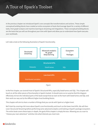
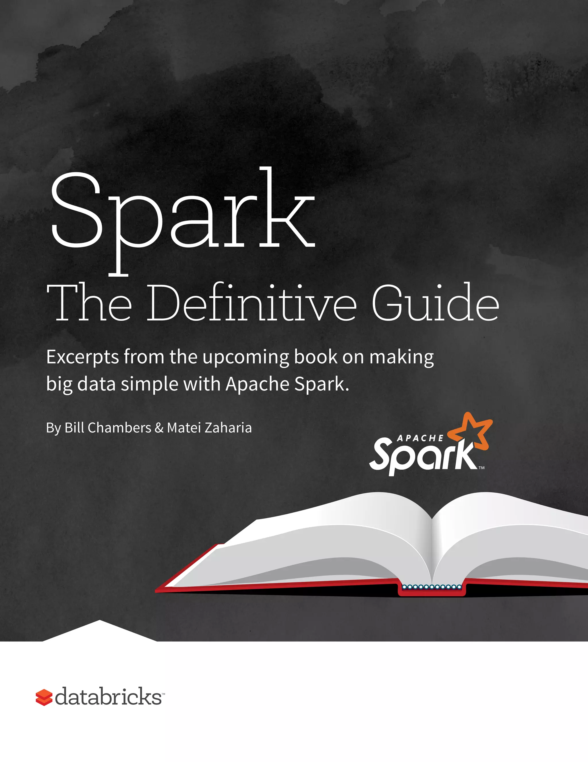
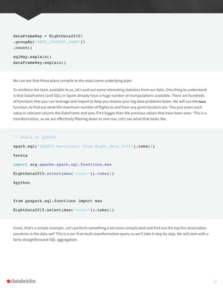
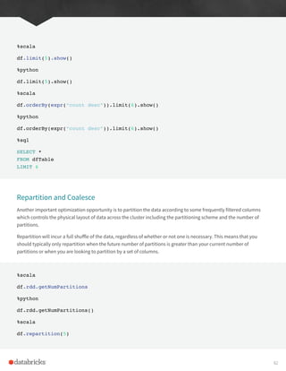
35. from pyspark.ml.feature import OneHotEncoder
encoder = OneHotEncoder()
.setInputCol(“day_of_week_index”)
.setOutputCol(“day_of_week_encoded”)
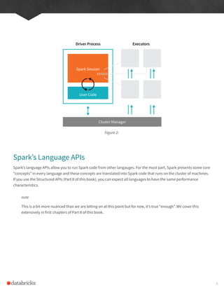
Each of these will result in a set of columns that we will “assemble” into a vector. All machine learning algorithms in
Spark take as input a Vector type, which must be a set of numerical values.
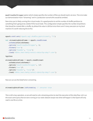
%scala
import org.apache.spark.ml.feature.VectorAssembler
val vectorAssembler = new VectorAssembler()
.setInputCols(Array(“UnitPrice”, “Quantity”, “day_of_week_encoded”))
.setOutputCol(“features”)
%python
from pyspark.ml.feature import VectorAssembler
vectorAssembler = VectorAssembler()
.setInputCols([“UnitPrice”, “Quantity”, “day_of_week_encoded”])
.setOutputCol(“features”)
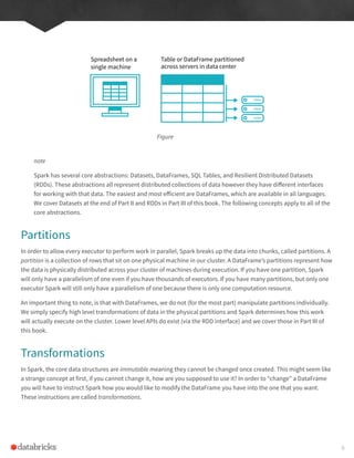
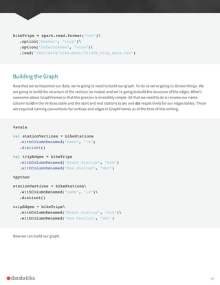
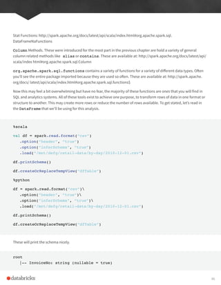
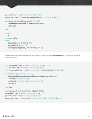
We can see that we have 4 key features, the price, the quantity, and the day of week. Now we’ll set this up into a
pipeline so any future data we need to transform can go through the exact same process.
%scala
import org.apache.spark.ml.Pipeline
val transformationPipeline = new Pipeline()
.setStages(Array(indexer, encoder, vectorAssembler))
%python
from pyspark.ml import Pipeline
35

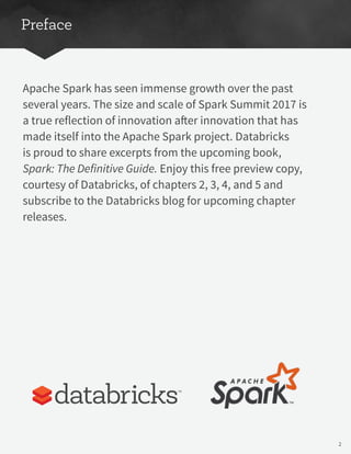
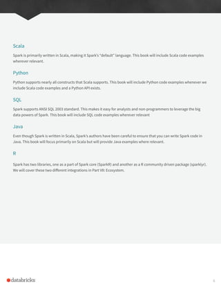
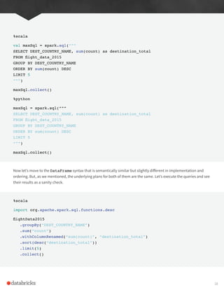
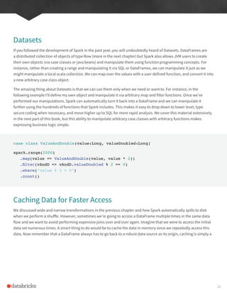
36. transformationPipeline = Pipeline()
.setStages([indexer, encoder, vectorAssembler])
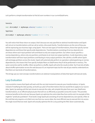
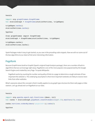
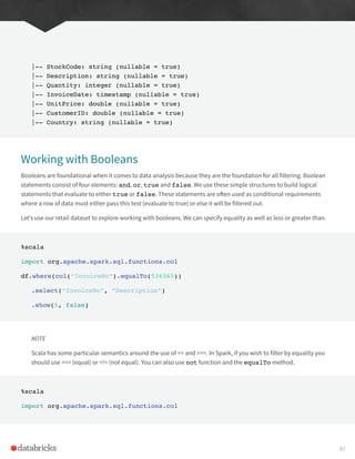
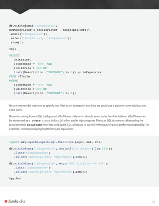
Now preparing for training is a two step process. We first need to fit our transformers to this dataset. We cover this in
depth, but basically our StringIndexer needs to know how many unique values there are to be index. Once those
exist, encoding is easy but Spark must look at all the distinct values in the column to be indexed in order to store
those values later on.
%scala
val fittedPipeline = transformationPipeline.fit(trainDataFrame)
%python
fittedPipeline = transformationPipeline.fit(trainDataFrame)
Once we fit the training data, we are now create to take that fitted pipeline and use it to transform all of our data in a
consistent and repeatable way.
%scala
val transformedTraining = fittedPipeline.transform(trainDataFrame)
%python
transformedTraining = fittedPipeline.transform(trainDataFrame)
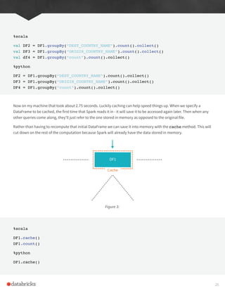
At this point, it’s worth mentioning that we could have included our model training in our pipeline. We chose not to
in order to demonstrate a use case for caching the data. At this point, we’re going to perform some hyperparameter
tuning on the model, since we do not want to repeat the exact same transformations over and over again, we’ll
instead cache our training set. This is worth putting it into memory because that will allow us to efficiently, and
repeatedly access it in an already transformed state. If you’re curious to see how much of a difference this makes,
skip this line and run the training without caching the data. Then try it after caching, you’ll see the results are (very)
significant.
transformedTraining.cache()
36

37. Now we have a training set, now it’s time to train the model. First we’ll import the relevant model that we’d like to use.
%scala
import org.apache.spark.ml.clustering.KMeans
val kmeans = new KMeans()
.setK(20)
.setSeed(1L)
%python
from pyspark.ml.clustering import KMeans
kmeans = KMeans()
.setK(20)
.setSeed(1L)
In Spark, training machine learning models is a two phase process. First we initialize an untrained model, then we
train it. There are always two types for every algorithm in MLlib’s DataFrame API. The algorithm Kmeans and then the
trained version which is a KMeansModel.
Algorithms and models in MLlib’s DataFrame API share roughly the same interface that we saw above with our
preprocessing transformers like the StringIndexer. This should come as no surprise because it makes training an entire
pipeline (which includes the model) simple. In our case we want to do things a bit more step by step, so we chose to
not do this at this point.
%scala
val kmModel = kmeans.fit(transformedTraining)
%python
kmModel = kmeans.fit(transformedTraining)
We can see the resulting cost at this point. Which is quite high, that’s likely because we didn’t necessary scale our data
or transform.
37

38. kmModel.computeCost(transformedTraining)
%scala
val transformedTest = fittedPipeline.transform(testDataFrame)
%python
transformedTest = fittedPipeline.transform(testDataFrame)
kmModel.computeCost(transformedTest)
Naturally we could continue to improve this model, layering more preprocessing as well as performing
hyperparameter tuning to ensure that we’re getting a good model. We leave that discussion for Part VI of this book,
where we discuss MLlib in depth.
Spark’s Ecosystem and Packages
Arguably one of the best parts about Spark is the ecosystem of packages and tools that the community has created.
Some of these tools even move into open source Spark as they mature and become widely used. The list of packages
is rather large at over 300 at the time of this writing and more are added frequently. A consolidated list of packages
can be found at https://spark-packages.org/ where any user can publish to this package repository and there are
numerous others that are not included.
The thing that brings together all Spark packages is that they allow for engineers to create optimized versions of Spark
for particular applications. GraphFrames is a perfect example, it makes Graph Analysis available on Spark’s Structured
APIs in ways that are much easier to use, and cross language, in a way that the lower level APIs do not support. There
are numerous other packages include many machine learning and deep learning packages that leverage Spark as the
core and extend the functionality.
Beyond these advanced analytics applications, packages exist to solve problems in particular verticals. Healthcare
and genomics have seen a particularly large surge in opportunity for big data applications. For example, the ADAM
Project leverages unique, internal optimizations to Spark’s Catalyst engine to provide a scalable API & CLI for genome
processing. Another package Hail is an opensource, scalable framework for exploring and analyzing genomic data.
Starting from sequencing or microarray data in VCF and other formats. Hail provides extremely sophisticated domain
relevant transformations to enable efficient analysis gigabyte-scale data on a laptop or terabyte-scale data on cluster.
There are countless other examples of the community coming together and creating projects to solve large scale
problems and we just wanted to discuss some of these projects and provide a short example of GraphFrames,
something that you’re likely able to apply to data right away.
38

39. GraphFrames
This section of the chapter will review a popular package, Graph- Frames, for advanced graph analytics.
You can see the GraphFrames package in the Spark-Packages repository. The version used here is
graphframes:graphframes:0.3.0-spark2.0-s_2.10.
Graph Analysis with GraphFrames
While a complete primer or graph analysis is out of scope for this chapter, the general idea is that graph theory and
processing are about defining relationships between different nodes and edges. Nodes or vertices are the units while
edges are the relationships that are defined between those. This object-relationship-object is a common way of
structing problems and GraphFrames makes it very easy to get started.
Setup & Data
Prior to reading in some data we’re going to need to install the GraphFrames Library. If you’re running this on
Databricks, you should do this by following this guide. Be sure to follow the directions for specifying the maven
coordinates. If you’re running this from the command line, you’ll want to specify the dependency when you launch
the console.
./bin/spark-shell --packages graphframes:graphframes:0.5.0-spark2.1-s_2.11
%scala
val bikeStations = spark.read.format(“csv”)
.option(“header”, “true”)
.option(“inferSchema”, “true”)
.load(“/mnt/defg/bike-data/201508_station_data.csv”)
val bikeTrips = spark.read.format(“csv”)
.option(“header”, “true”)
.option(“inferSchema”, “true”)
.load(“/mnt/defg/bike-data/201508_trip_data.csv”)
%python
bikeStations = spark.read.format(“csv”)
.option(“header”, “true”)
.option(“inferSchema”, “true”)
.load(“/mnt/defg/bike-data/201508_station_data.csv”)
39

40. bikeTrips = spark.read.format(“csv”)
.option(“header”, “true”)
.option(“inferSchema”, “true”)
.load(“/mnt/defg/bike-data/201508_trip_data.csv”)
Building the Graph
Now that we’ve imported our data, we’re going to need to build our graph. To do so we’re going to do two things. We
are going to build the structure of the vertices (or nodes) and we’re going to build the structure of the edges. What’s
awesome about GraphFrames is that this process is incredibly simple. All that we need to do is rename our name
column to id in the Vertices table and the start and end stations to src and dst respectively for our edges tables. These
are required naming conventions for vertices and edges in GraphFrames as of the time of this writing.
%scala
val stationVertices = bikeStations
.withColumnRenamed(“name”, “id”)
.distinct()
val tripEdges = bikeTrips
.withColumnRenamed(“Start Station”, “src”)
.withColumnRenamed(“End Station”, “dst”)
%python
stationVertices = bikeStations
.withColumnRenamed(“name”, “id”)
.distinct()
tripEdges = bikeTrips
.withColumnRenamed(“Start Station”, “src”)
.withColumnRenamed(“End Station”, “dst”)
Now we can build our graph.
40

41. %scala
import org.graphframes.GraphFrame
val stationGraph = GraphFrame(stationVertices, tripEdges)
tripEdges.cache()
stationVertices.cache()
%python
from graphframes import GraphFrame
stationGraph = GraphFrame(stationVertices, tripEdges)
tripEdges.cache()
stationVertices.cache()
Spark Packages make it easy to get started, as you saw in the preceding code snippets. Now we will run some out of
the box algorithms to our data to find some interesting information.
PageRank
Because GraphFrames build on GraphX (Spark’s original Graph Analysis package), there are a number of built-in
algorithms that we can leverage right away. PageRank is one of the more popular ones popularized by the Google
Search Engine and created by Larry Page. To quote Wikipedia:
PageRank works by counting the number and quality of links to a page to determine a rough estimate of how
important the website is. The underlying assumption is that more important websites are likely to receive more
links from other websites.
What’s awesome about this concept is that it readily applies to any graph type structure be them web pages or bike
stations. Let’s go ahead and run PageRank on our data.
%scala
import org.apache.spark.sql.functions.{desc, col}
val ranks = stationGraph.pageRank.resetProbability(0.15).maxIter(10).run()
ranks.vertices.orderBy(desc(“pagerank”)).take(5)
%python
41

42. from pyspark.sql.functions import desc
ranks = stationGraph.pageRank(maxIter=10).resetProbability(0.15).run()
ranks.vertices.orderBy(desc(“pagerank”)).take(5)
We can see that the Caltrain stations seem to have significance, and this makes sense. Train stations are natural
connectors and likely one of the most popular uses of these bike share programs to get you from A to B in a way that
you don’t need a car!
Trips From Station to Station
One question you might ask is what are the most common destinations in the dataset from location to location. We
can do this by performing a grouping operator and adding the edge counts together. This will yield a new graph except
each edge will now be the sum of all of the semantically same edges. Think about it this way: we have a number of
trips that are the exact same from station A to station B, we just want to count those up!
In the below query you’ll see that we’re going to grab the station to station trips that are most common and print out
the top 10.
%scala
stationGraph
.edges
.groupBy(“src”, “dst”)
.count()
.orderBy(desc(“count”))
.limit(10)
.show()
%python
stationGraph
.edges
.groupBy(“src”, “dst”)
.count()
.orderBy(desc(“count”))
.limit(10)
.show()
42

43. GraphFrames provides a simple to use interface to get value out or graph structured data right away. Other Spark
Packages provide similar functionality, making it simple to leverage hyper-optimized packages for a variety of
different data sources, algorithms and applications, and much more.
Conclusion
We hope this chapter showed you a variety of the different ways that you can apply Spark to your own business and
technical challenges. Spark’s simple, robust programming model make it easy to apply to a large number of problems
and the vast array of packages that have crept up around it created by hundreds of different people are a true
testament to Spark’s ability to apply robustly to a number of business problems and challenges. As the ecosystem and
community grows, it’s likely that more and more packages will continue to crop up. We look forward to seeing what
the community has in store!
The rest of this book will provide deeper dives into the product areas in the following image.
You may read the rest of the book anyway that you wish, we find that most people hop from area to area as they hear
terminology or want to apply Spark to certain problems they’re facing.
Figure
Structured APIs
DataFrames SQL
Datasets
Structured
streaming
Advanced analytics
ML graph
Deep learning
Ecosystem
+
Packages
Low level APIs
Distributed variables RDDs
43

44. Structured API Overview
This part of the book will be a deep dive into Spark’s Structured APIs. These APIs are core to Spark and likely
where you’ll spend a lot of time with Spark. The Structured APIs are a way of manipulating all sorts of data, from
unstructured log files, to semi-structured CSV files, and highly structured Parquet files. These APIs refer to three core
types of distributed collection APIs.
• Datasets
• DataFrames
• SQL Views and Tables
This part of the book will cover all the core ideas behind the Structured APIs and how to apply them to your big data
challenges. Although distinct in the book, the vast majority of these user-facing operations apply to both batch as well
as streaming computation. Meaning that when you work with the Structured APIs, it should be simple to migrate from
batch to streaming with little to no effort (or the opposite).
The Structured APIs are the fundamental abstraction that you will leverage to write the majority of your data flows.
Thus far in this book we have taken a tutorial-based approach, meandering our way through much of what Spark
has to offer. In this section, we will perform a deeper dive. This introductory chapter will introduce the fundamental
concepts that you should understand: the typed and untyped APIs (and their differences); how to work with different
kinds of data using the structured APIs; and deep dives into different data flows with Spark. The later chapters will
provide operation based information.
BOX Before proceeding, let’s review the fundamental concepts and definitions that we covered in the previous
section. Spark is a distributed programming model where the user specifies transformations, which build
up a directed acyclic- graph of instructions, and actions, which begin the process of executing that graph of
instructions, as a single job, by breaking it down into stages and tasks to execute across the cluster. The way
we store data on which to perform transformations and actions are DataFrames and Datasets. To create a
new DataFrame or Dataset, you call a transformation. To start computation or convert to native language
types, you call an action.
DataFrames and Datasets
In Section I, we talked all about DataFrames. Spark has two notions of “structured” collections: DataFrames and
Datasets. We will touch on the (nuanced) differences shortly but let’s define what they both represent first.
To the user, DataFrames and Datasets are (distributed) table like collections with well-defined rows and columns.
Each column must have the same number of rows as all the other columns (although you can use null to specify the
44

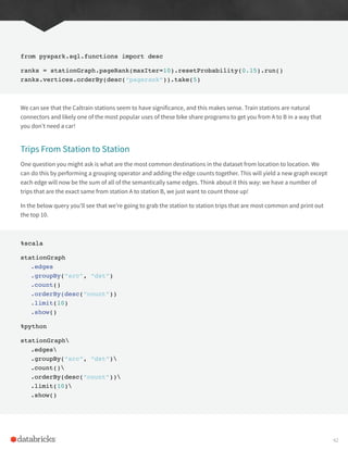
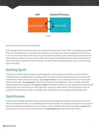
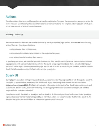
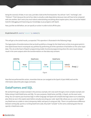
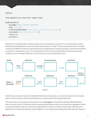
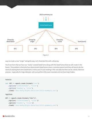
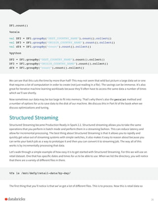
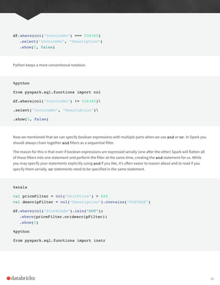
45. lack of a value) and columns have type information that must be consistent for every row in the collection. To Spark,
DataFrames and Datasets represent immutable, lazily-evaluated plans that specify what operations to apply to
data residing at a location to generate some output. When we perform an action on a DataFrame we instruct Spark
to perform the actual transformations and return the result. These represent plans of how to manipulate rows and
columns to compute the user’s desired result. Let’s go over rows and column to more precisely define those concepts.
note
Tables and views are basically the same thing as DataFrames. We just execute SQL against them instead of
DataFrame code. We cover all of this in the Spark SQL Chapter later on in Part II of this book.
In order to do that,we should talk about schemas, the way we define the types of data we’re storing in this
distributed collection.
Schemas
A schema defines the column names and types of a DataFrame. Users can define schemas manually or users can
read a schema from a data source (often called schema on read)|. Now that we know what defines DataFrames and
Datasets and how they get their structure, via a Schema, let’s see an overview of all of the types.
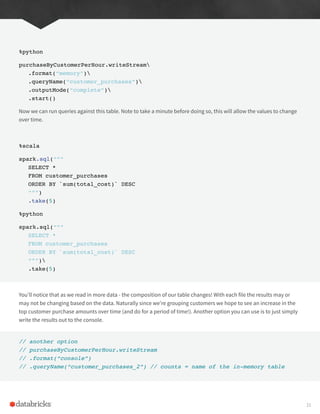
Overview of Structured Spark Types
Spark is effectively a programming language of its own. Internally, Spark uses an engine called Catalyst that maintains
its own type information through the planning and processing of work. This may seem like overkill, but it doing so,
this opens up a wide variety of execution optimizations that make significant differences. Spark types map directly
to the different language APIs that Spark maintains and there exists a lookup table for each of these in each of Scala,
Java, Python, SQL, and R. Even if we use Spark’s Structured APIs from Python or R, the majority of our manipulations
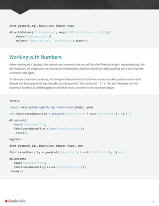
will operate strictly on Spark types, not Python types. For example, the below code does not perform addition in Scala
or Python, it actually performs addition purely in Spark.
%scala
val df = spark.range(500).toDF(“number”)
df.select(df.col(“number”) + 10)
// org.apache.spark.sql.DataFrame = [(number + 10): bigint]
%python
df = spark.range(500).toDF(“number”)
df.select(df[“number”] + 10)
# DataFrame[(number + 10): bigint]
45

46. This addition operation happens because Spark will convert an expression expressed in an input language to Spark’s
internal Catalyst representation of that same type information. Now that we’ve clearly defined that Spark maintains
its own type information, let’s dive into some of the nuanced differences of the output you may see when you’re
working with Spark.
In essence, within the Structured APIs, there are two more APIs, the “untyped” DataFrames and the “typed” Datasets.
To say that DataFrames are untyped is a bit of a misnomer, they have types but Spark maintains them completely and
only checks whether those types line up to those specified in the schema at runtime. Datasets, on the other hand,
check whether or not types conform to the specification at compile time. Datasets are only available to JVM based
languages (Scala and Java) and we specify types with case classes or Java beans.
For the most part, you’re likely to work with DataFrames and we cover DataFrames extensively in this part of the book.
To Spark in Scala, DataFrames are simply Datasets of Type Row. The “Row” type is Spark’s internal representation of
its optimized in memory format for computation. This format makes for highly specialized and efficient computation
because rather than leveraging JVM types which can cause high garbage collection and object instantiation costs,
Spark can operate on its own internal format without incurring any of those costs. To Spark in Python, there is no such
thing as a Dataset, everything is a DataFrame.
note
This internal format is well covered in numerous Spark talks and for the more general audience we will abstain
from going into the implementation. For the curious there are some excellent talks by Josh Rosen of Databricks
and Herman van Hovell of Databricks about their work in the development of Spark’s Catalyst engine.
Defining DataFrames, types, and Schemas is always a mouthful and takes sometime to digest. What most need to
know is that when you’re using DataFrames, you’re leverage Spark’s optimized internal format. This format applies
the same efficiency gains to all of Spark’s language APIs. For those that need strict compile time checking, they should
see the Datasets Chapter at the end of Part II of this book to learn more about them and how to use them.
Let’s move onto some more friendly and approachable concepts, columns and rows.
Columns
For now, all you need to understand about columns is that they can represent a simple type like an integer or string,
a complex types like an array or map, or a null value. Spark tracks all of this type information to you and has a variety
of ways that you can transform columns. Columns are discussed extensively in the next chapter but for the most part
you can think about Spark Column types as columns in a table.
46

47. Rows
There are two ways of getting data into Spark, through Rows and Encoders. Row objects are the most general way of
getting data into, and out of, Spark and are available in all languages. Each record in a DataFrame must be of Row type
as we can see when we collect the following DataFrames. This row is the internal, optimized format that we reference
above.
%scala
spark.range(2).toDF().collect()
%python
spark.range(2).collect()
Spark Types
We mentioned above Spark has a large number of internal type representations. We include a handy reference table
on the next several pages in order for you to most easily reference what type, in your specific language, lines up with
the type in Spark.
Before getting to those tables, let’s talk about how we instantiate or declare a column to be of a certain type.
To work with the correct Scala types:
import org.apache.spark.sql.types._
val b = ByteType()
To work with the correct Java types you should use the factory methods in the following package:
import org.apache.spark.sql.types.DataTypes;
ByteType x = DataTypes.ByteType();
Python types at time have certain requirements (like the listed requirement for ByteType below.To work with the
47

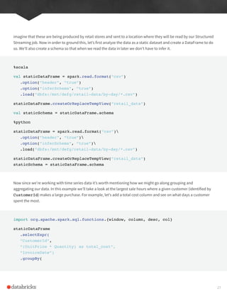
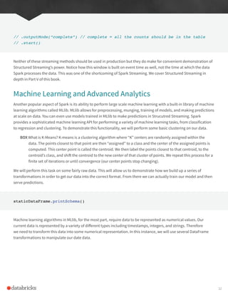
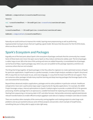
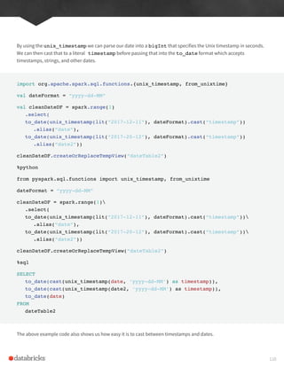
48. correct Python types:
from pyspark.sql.types import *
b = byteType()
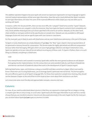
Scala Type Reference
Data type Value type in Scala API to access or create a data type
ByteType
ShortType
IntegerType
LongType
FloatType
DoubleType
DecimalType
StringType
BinaryType
BooleanType
TimestampType
DateType
ArrayType
MapType
StructType
Struct Field
Byte
Short
Type
Long
Float
Double
java.math.BigDecimal
String
Array [Byte]
Boolean
java.sql.Timestamp
java.sql.Date
scala.collection.Seq
scala.collection.Map
org.apache.spark.sql.Row
The value type in Scala of the data
type of this field (For example, Int
for a StructField with the data type
IntegerType)
ByteType
ShortType
IntegerType
LongType
FloatType
DoubleType
DecimalType
StringType
BinaryType
BooleanType
TimestampType
DateType
ArrayType(elementType, [containsNull]) Note:
The default value of containsNull is true.
MapType (keyType, valueType,
[valuecontainsNull]) Note: The default value
of valuecontainsNull is true.
StructType (fields) Note: fields is a Seq of
StructFields. Also, two fields with the same
name are not allowed.
StructField(name, dataType, [nullable]) Note:
The default value of nullable is true.
48

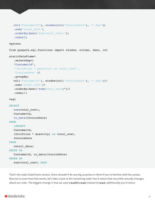
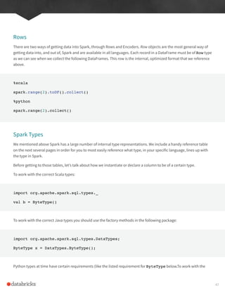
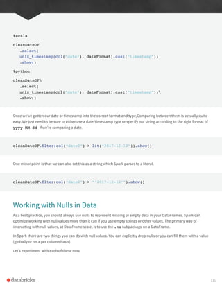
49. Java Type Reference
Data type Value type in Java API to access or create a data type
ByteType
ShortType
IntegerType
LongType
FloatType
DoubleType
DecimalType
StringType
BinaryType
BooleanType
TimestampType
DateType
ArrayType
MapType
StructType
Struct Field
byte or Byte
short or Short
integer or Integer
long or Long
float or Float
double or Double
java.math.BigDecimal
String
byte []
boolean or Boolean
java.sql.Timestamp
java.sql.Date
java.util.List
java.util.Map
org.apache.spark.sql.Row
Field value type in Java of the data
type of this field (For example, int
for a StructField with the data type
IntegerType)
DataTypes.ByteType
DataTypes.ShortType
DataTypes.IntegerType
DataTypes.LongType
DataTypes.FloatType
DataTypes.DoubleType
DataTypes.DecimalType
DataTypes.StringType
DataTypes.BinaryType
DataTypes.BooleanType
DataTypes.TimestampType
DataTypes.DateType
DataTypes.createArrayType(elementType)
Note: The value of containsNull will be true
DataTypes.createArrayType(elementType,
containsNull).
DataTypes.createMapType(keyType,
valueType) Note: The value of
valueContainsNull will be true. DataTypes.
createMapType(keyType, valueType,
valueContainsNull)
DataTypes.createStructType(fields) Note:
fields is a List or an array of StructFields.
Also, two fields with the same name are not
allowed.
DataTypes.createStructField(name, dataType,
nullable)
49

50. Python Type Reference
Data type Value type in Python API to access or create a data type
ByteType
ShortType
IntegerType
LongType
FloatType
DoubleType
DecimalType
StringType
BinaryType
BooleanType
TimestampType
DateType
ArrayType
MapType
StructType
intor long Note: Numbers will be
converted to 1-byte signed integer
numbers at runtime. Please make sure
that numbers are within the range of
-128 to 127.
intor long Note: Numbers will be
converted to 2-byte signed integer
numbers at runtime. Please make sure
that numbers are within the range of
-32768 to 32767.
type long
long Note: Numbers will be
converted to 8-byte signed integer
numbers at runtime. Please make
sure that numbers are within the
range of -9223372036854775808 to
9223372036854775807. Otherwise,
please convert data to decimal.Decimal
and use DecimalType.
float Note: Numbers will be converted
to 4-byte single-precision floating point
numbers at runtime.
float
decimal.Decimal
string
bytearray
bool
datetime.datetime
datetime.date
list, tuple, or array
dict
Field value type in Java of the data
type of this field (For example, int
for a StructField with the data type
IntegerType)
ByteType()
ShortType()
IntegerType()
LongType()
FloatType()
DoubleType()
DecimalType()
StringType()
BinaryType()
BooleanType()
TimestampType()
DateType()
ArrayType(elementType, [containsNull]) Note:
The default value of containsNull is True.
MapType(keyType, valueType,
[valueContainsNull]) Note: The default value
of valueContainsNull is True.
StructType(fields) Note: fields is a Seq of
StructFields. Also, two fields with the same
name are not allowed.
50

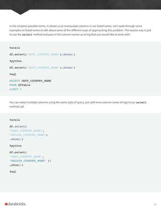
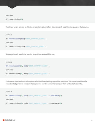
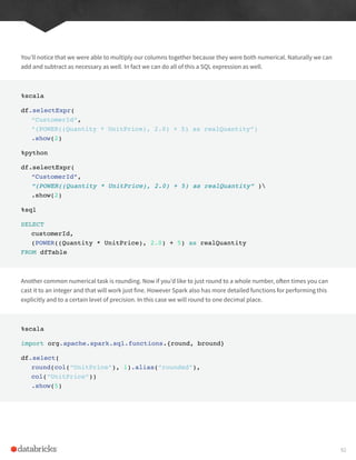
51. SQL
Datasets
DataFrames
Catalyst optimizer Physical plan
Python Type Reference (cont.)
Data type Value type in Python API to access or create a data type
Struct Field The value type in Python of the data
type of this field (For example, Int
for a StructField with the data type
IntegerType)
StructField(name, dataType, [nullable]) Note:
The default value of nullable is True.
It’s worth keeping in mind that the types may change over time and there may be truncation (especially when
dealing with certain languages lack of precise data types). It’s always worth checking the documentation for the most
up to date information.
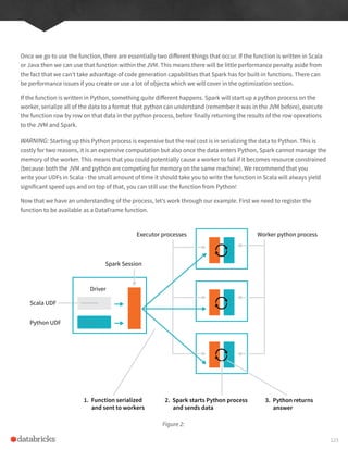
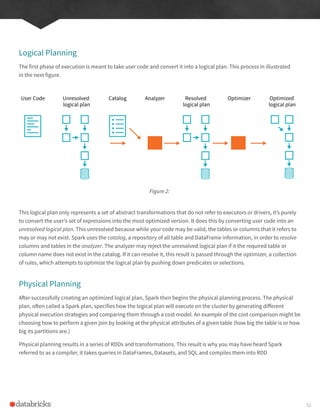
Overview of Structured API Execution
In order to help you understand (and potentially debug) the process of writing and executing code on clusters, let’s
walk through the execution of a single structured API query from user code to executed code. As an overview the
steps are:
1. Write DataFrame/Dataset/SQL Code
2. If valid code, Spark converts this to a Logical Plan
3. Spark transforms this Logical Plan to a Physical Plan
4. Spark then executes this Physical Plan on the cluster
To execute code, we have to write code. This code is then submitted to Spark either through the console or via a
submitted job. This code then passes through the Catalyst Optimizer which decides how the code should be executed
and lays out a plan for doing so, before finally the code is run and the result is returned to the user.
Figure
51

52. Logical Planning
The first phase of execution is meant to take user code and convert it into a logical plan. This process in illustrated
in the next figure.
This logical plan only represents a set of abstract transformations that do not refer to executors or drivers, it’s purely
to convert the user’s set of expressions into the most optimized version. It does this by converting user code into an
unresolved logical plan. This unresolved because while your code may be valid, the tables or columns that it refers to
may or may not exist. Spark uses the catalog, a repository of all table and DataFrame information, in order to resolve
columns and tables in the analyzer. The analyzer may reject the unresolved logical plan if it the required table or
column name does not exist in the catalog. If it can resolve it, this result is passed through the optimizer, a collection
of rules, which attempts to optimize the logical plan by pushing down predicates or selections.
Physical Planning
After successfully creating an optimized logical plan, Spark then begins the physical planning process. The physical
plan, often called a Spark plan, specifies how the logical plan will execute on the cluster by generating different
physical execution strategies and comparing them through a cost model. An example of the cost comparison might be
choosing how to perform a given join by looking at the physical attributes of a given table (how big the table is or how
big its partitions are.)
Physical planning results in a series of RDDs and transformations. This result is why you may have heard Spark
referred to as a compiler, it takes queries in DataFrames, Datasets, and SQL and compiles them into RDD
Figure 2:
Catalog
Unresolved
logical plan
Analyzer Resolved
logical plan
Optimizer Optimized
logical plan
User Code
52

53. transformations for you.
Execution
Upon selecting a physical plan, Spark runs all of this code over RDDs, the lower-level programming interface of Spark
covered in Part III. Spark performs further optimizations by, at runtime, generating native Java Bytecode that can
remove whole tasks or stages during execution. Finally the result is returned to the user.
Figure
Optimized
logical plan
Physical plans Best physical plan Executed on cluster
Cost model
53

54. Basic Structured Operations
Chapter Overview
In the previous chapter we introduced the core abstractions of the Structured API. This chapter will move away from
the architectural concepts and towards the tactical tools you will use to manipulate DataFrames and the data within
them. This chapter will focus exclusively on single DataFrame operations and avoid aggregations, window functions,
and joins which will all be discussed in depth later in this section.
Definitionally, a DataFrame consists of a series of records (like rows in a table), that are of type Row, and a number
of columns (like columns in a spreadsheet) that represent an computation expression that can performed on each
individual record in the dataset. The schema defines the name as well as the type of data in each column. The
partitioning of the DataFrame defines the layout of the DataFrame or Dataset’s physical distribution across the cluster.
The partitioning scheme defines how that is broken up, this can be set to be based on values in a certain column or
non-deterministically.
Let’s define a DataFrame to work with.
%scala
val df = spark.read.format(“json”)
.load(“/mnt/defg/flight-data/json/2015-summary.json”)
%python
df = spark.read.format(“json”)
.load(“/mnt/defg/flight-data/json/2015-summary.json”)
We discussed that a DataFame will have columns, and we use a “schema” to view all of those. We can run the
following command in Scala or in Python.
df.printSchema()
The schema ties the logical pieces together and is the starting point to better understand DataFrames.
54

55. Schemas
A schema defines the column names and types of a DataFrame. We can either let a data source define the schema
(called schema on read) or we can define it explicitly ourselves.
NOTE
Deciding whether or not you need to define a schema prior to reading in your data depends your use case. Often
times for ad hoc analysis, schema on read works just fine (although at times it can be a bit slow with plain text
file formats like csv or json). However, this can also lead to precision issues like a long type incorrectly set as an
integer when reading in a file. When using Spark for production ETL, it is often a good idea to define your schemas
manually, especially when working with untyped data sources like csv and json because schema inference can
vary depending on the type of data that you read in.
Let’s start with a simple file we saw in the previous chapter and let the semistructured nature of line-delimited JSON
define the structure. This data is flight data from the United States Bureau of Transportation statistics.
%scala
spark.read.format(“json”)
.load(“/mnt/defg/flight-data/json/2015-summary.json”)
.schema
Scala will return:
org.apache.spark.sql.types.StructType = ...
StructType(StructField(DEST_COUNTRY_NAME,StringType,true),
StructField(ORIGIN_COUNTRY_NAME,StringType,true),
StructField(count,LongType,true))
%python
spark.read.format(“json”)
.load(“/mnt/defg/flight-data/json/2015-summary.json”)
.schema
55

56. Python will return:
StructType(List(StructField(DEST_COUNTRY_NAME,StringType,true),
StructField(ORIGIN_COUNTRY_NAME,StringType,true),
StructField(count,LongType,true)))
A schema is a StructType made up of a number of fields, StructFields, that have a name, type, and a boolean
flag which specifies whether or not that column can contain missing or null values. Schemas can also contain other
StructType (Spark’s complex types). We will see this in the next chapter when we discuss working with complex
types.
Here’s how to create, and enforce a specific schema on a DataFrame. If the types in the data (at runtime), do not
match the schema. Spark will throw an error.
%scala
import org.apache.spark.sql.types.{StructField, StructType, StringType, LongType}
val myManualSchema = new StructType(Array(
new StructField(“DEST_COUNTRY_NAME”, StringType, true),
new StructField(“ORIGIN_COUNTRY_NAME”, StringType, true),
new StructField(“count”, LongType, false) // just to illustrate flipping
this flag
))
val df = spark.read.format(“json”)
.schema(myManualSchema)
.load(“/mnt/defg/flight-data/json/2015-summary.json”)
Here’s how to do the same in Python.
%python
from pyspark.sql.types import StructField, StructType, StringType, LongType
56

57. myManualSchema = StructType([
StructField(“DEST_COUNTRY_NAME”, StringType(), True),
StructField(“ORIGIN_COUNTRY_NAME”, StringType(), True),
StructField(“count”, LongType(), False)
])
df = spark.read.format(“json”)
.schema(myManualSchema)
.load(“/mnt/defg/flight-data/json/2015-summary.json”)
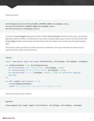
As discussed in the previous chapter, we cannot simply set types via the per language types because Spark maintains
its own type information. Let’s now discuss what schemas define, columns.
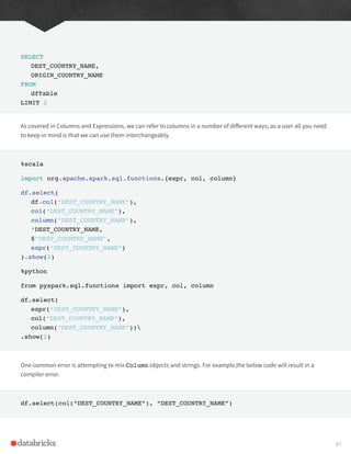
Columns and Expressions
To users, columns in Spark are similar to columns in a spreadsheet, R dataframe, pandas DataFrame. We can select,
manipulate, and remove columns from DataFrames and these operations are represented as expressions.
To Spark, columns are logical constructions that simply represent a value computed on a per-record basis by means
of an expression. This means, in order to have a real value for a column, we need to have a row, and in order to
have a row we need to have a DataFrame. This means that we cannot manipulate an actual column outside of a
DataFrame, we can only manipulate a logical column’s expressions then perform that expression within the context of
a DataFrame.
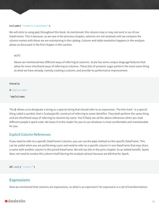
Columns
There are a lot of different ways to construct and or refer to columns but the two simplest ways are with the col or
column functions. To use either of these functions, we pass in a column name.
%scala
import org.apache.spark.sql.functions.{col, column}
col(“someColumnName”)
column(“someColumnName”)
%python
from pyspark.sql.functions import col, column
col(“someColumnName”)
57

58. column(“someColumnName”)
We will stick to using col throughout this book. As mentioned, this column may or may not exist in our of our
DataFrames. This is because, as we saw in the previous chapter, columns are not resolved until we compare the
column names with those we are maintaining in the catalog. Column and table resolution happens in the analyzer
phase as discussed in the first chapter in this section.
NOTE
Above we mentioned two different ways of referring to columns. Scala has some unique language features that
allow for more shorthand ways of referring to columns. These bits of syntactic sugar perform the exact same thing
as what we have already, namely creating a column, and provide no performance improvement.
%scala
$”myColumn”
‘myColumn
The $ allows us to designate a string as a special string that should refer to an expression. The tick mark ‘ is a special
thing called a symbol, that is Scalaspecific construct of referring to some identifier. They both perform the same thing
and are shorthand ways of referring to columns by name. You’ll likely see all the above references when you read
different people’s spark code. We leave it to the reader for you to use whatever is most comfortable and maintainable
for you.
Explicit Column References
If you need to refer to a specific DataFrame’s column, you can use the col method on the specific DataFrame. This
can be useful when you are performing a join and need to refer to a specific column in one DataFrame that may share
a name with another column in the joined DataFrame. We will see this in the joins chapter. As an added benefit, Spark
does not need to resolve this column itself (during the analyzer phase) because we did that for Spark.
df.col(“count”)
Expressions
Now we mentioned that columns are expressions, so what is an expression? An expression is a set of transformations
58

59. on one or more values in a record in a DataFrame. Think of it like a function that takes as input one or more column
names, resolves them and then potentially applies more expressions to create a single value for each record in the
dataset. Importantly, this “single value” can actually be a complex type like a Map type or Array type.
In the simplest case, an expression, created via the expr function, is just a DataFrame column reference.
import org.apache.spark.sql.functions.{expr, col}
In this simple instance, expr(“someCol”) is equivalent to col(“someCol”).
Columns as Expressions
Columns provide a subset of expression functionality. If you use col() and wish to perform transformations on
that column, you must perform those on that column reference. When using an expression, the expr function can
actually parse transformations and column references from a string and can subsequently be passed into further
transformations. Let’s look at some examples.
expr(“someCol - 5”) is the same transformation as performing col(“someCol”) - 5 or even
expr(“someCol”) - 5. That’s because Spark compiles these to a logical tree specifying the order of operations.
This might be a bit confusing at first, but remember a couple of key points.
1. Columns are just expressions.
2. Columns and transformations of those column compile to the same logical plan as parsed expressions.
Let’s ground this with an example.
(((col(“someCol”) + 5) * 200) - 6) < col(“otherCol”)
59

60. Figure 1:
Figure 1 shows an illustration of that logical tree.
This might look familiar because it’s a directed acyclic graph. This graph is represented equivalently with the
following code.
%scala
import org.apache.spark.sql.functions.expr
expr(“(((someCol + 5) * 200) - 6) < otherCol”)
%python
from pyspark.sql.functions import expr
expr(“(((someCol + 5) * 200) - 6) < otherCol”)
This is an extremely important point to reinforce. Notice how the previous expression is actually valid SQL code
as well, just like you might put in a SELECT statement? That’s because this SQL expression and the previous
DataFrame code compile to the same underlying logical tree prior to execution. This means you can write your
expressions as DataFrame code or as SQL expressions and get the exact same benefits. You likely saw all of this in the
first chapters of the book and we covered this more extensively in the Overview of the Structured APIs chapter.
Some col
+
Other col
6
200
5
*
_
<
60

61. Accessing a DataFrame’s Columns
Sometimes you’ll need to see a DataFrame’s columns, you can do this by doing something like printSchema however
if you want to programmatically access columns, you can use the columns method to see all columns listed.
spark.read.format(“json”)
.load(“/mnt/defg/flight-data/json/2015-summary.json”)
.columns
Records and Rows
In Spark, a record or row makes up a “row” in a DataFrame. A logical record or row is an object of type Row. Row
objects are the objects that column expressions operate on to produce some usable value. Row objects represent
physical byte arrays. The byte array interface is never shown to users because we only use column expressions to
manipulate them.
You’ll notice collections that return values will always return one or more Row types.
NOTE
we will use lowercase “row” and “record” interchangeably in this chapter, with a focus on the latter. A capitalized
“Row” will refer to the Row object. We can see a row by calling first on our DataFrame.
%scala
df.first()
%python
df.first()
Creating Rows
You can create rows by manually instantiating a Row object with the values that below in each column. It’s important
to note that only DataFrames have schema. Rows themselves do not have schemas. This means if you create a Row
61

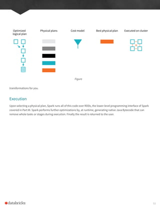
62. manually, you must specify the values in the same order as the schema of the DataFrame they may be appended to.
We will see this when we discuss creating DataFrames.
%scala
import org.apache.spark.sql.Row
val myRow = Row(“Hello”, null, 1, false)
%python
from pyspark.sql import Row
myRow = Row(“Hello”, None, 1, False)
Accessing data in rows is equally as easy. We just specify the position. However because Spark maintains its own type
information, we will have to manually coerce this to the correct type in our respective language.
For example in Scala, we have to either use the helper methods or explicitly coerce the values.
%scala
myRow(0) // type Any
myRow(0).asInstanceOf[String] // String
myRow.getString(0) // String
myRow.getInt(2) // String
There exist one of these helper functions for each corresponding Spark and Scala type. In Python, we do not have to
worry about this, Spark will automatically return the correct type by location in the Row Object.
%python
myRow[0]
myRow[2]
62

63. You can also explicitly return a set of Data in the corresponding JVM objects by leverage the Dataset APIs. This is
covered at the end of the Structured API section.
DataFrame Transformations
Now that we briefly defined the core parts of a DataFrame, we will move onto manipulating DataFrames. When
working with individual DataFrames there are some fundamental objectives. These break down into several core
operations.
• We can add rows or columns
• We can remove rows or columns
• We can transform a row into a column (or vice versa)
• We can change the order of rows based on the values in columns
Luckily we can translate all of these into simple transformations, the most common being those that take one column,
change it row by row, and then return our results.
Figure
Creating DataFrames
As we saw previously, we can create DataFrames from raw data sources. This is covered extensively in the Data
Sources chapter however we will use them now to create an example DataFrame. For illustration purposes later
in this chapter, we will also register this as a temporary view so that we can query it with SQL.
Remove columns or rows
Row into a column
or column into a row
Add rows or columns
Sort data by values in rows
63

64. %scala
val df = spark.read.format(“json”)
.load(“/mnt/defg/flight-data/json/2015-summary.json”)
df.createOrReplaceTempView(“dfTable”)
%python
df = spark.read.format(“json”)
.load(“/mnt/defg/flight-data/json/2015-summary.json”)
df.createOrReplaceTempView(“dfTable”)
We can also create DataFrames on the fly by taking a set of rows and converting them to a DataFrame.
%scala
import org.apache.spark.sql.Row
import org.apache.spark.sql.types.{StructField, StructType,
StringType, LongType}
val myManualSchema = new StructType(Array(
new StructField(“some”, StringType, true),
new StructField(“col”, StringType, true),
new StructField(“names”, LongType, false) // just to illustrate flipping
this flag
))
val myRows = Seq(Row(“Hello”, null, 1L))
val myRDD = spark.sparkContext.parallelize(myRows)
val myDf = spark.createDataFrame(myRDD, myManualSchema)
myDf.show()
NOTE: In Scala we can also take advantage of Spark’s implicits in the console (and if you import them in your jar
code), by running to DF on a Seq type. This does not play well with null types, so it’s not necessarily recommended for
production use cases.
64

65. %scala
val myDF = Seq((“Hello”, 2, 1L)).toDF()
%python
from pyspark.sql import Row
from pyspark.sql.types import StructField, StructType,
StringType, LongType
myManualSchema = StructType([
StructField(“some”, StringType(), True),
StructField(“col”, StringType(), True),
StructField(“names”, LongType(), False)
])
myRow = Row(“Hello”, None, 1)
myDf = spark.createDataFrame([myRow], myManualSchema)
myDf.show()
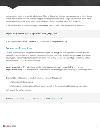
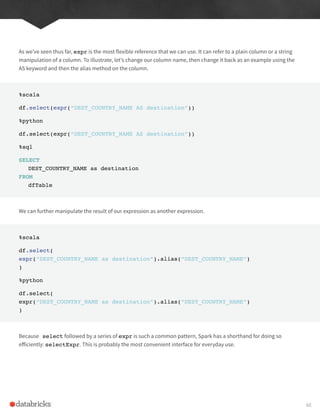
Now that we know how to create DataFrames, let’s go over their most useful methods that you’re going to be using
are: the select method when you’re working with columns or expressions and the selectExpr method when
you’re working with expressions in strings. Naturally some transformations are not specified as a methods on
columns, therefore there exists a group of functions found in the org.apache.spark.sql.functions package.
With these three tools, you should be able to solve the vast majority of transformation challenges that you may
encourage in DataFrames.
Select & SelectExpr
Select and SelectExpr allow us to do the DataFrame equivalent of SQL queries on a table of data.
SELECT * FROM dataFrameTable
SELECT columnName FROM dataFrameTable
SELECT columnName * 10, otherColumn, someOtherCol as c FROM dataFrameTable
65

66. In the simplest possible terms, it allows us to manipulate columns in our DataFrames. Let’s walk through some
examples on DataFrames to talk about some of the different ways of approaching this problem. The easiest way is just
to use the select method and pass in the column names as string that you would like to work with.
%scala
df.select(“DEST_COUNTRY_NAME”).show(2)
%python
df.select(“DEST_COUNTRY_NAME”).show(2)
%sql
SELECT DEST_COUNTRY_NAME
FROM dfTable
LIMIT 2
You can select multiple columns using the same style of query, just add more column name strings to our select
method call.
%scala
df.select(
“DEST_COUNTRY_NAME”,
“ORIGIN_COUNTRY_NAME”)
.show(2)
%python
df.select(
“DEST_COUNTRY_NAME”,
“ORIGIN_COUNTRY_NAME” )
.show(2)
%sql
66

67. SELECT
DEST_COUNTRY_NAME,
ORIGIN_COUNTRY_NAME
FROM
dfTable
LIMIT 2
As covered in Columns and Expressions, we can refer to columns in a number of different ways; as a user all you need
to keep in mind is that we can use them interchangeably.
%scala
import org.apache.spark.sql.functions.{expr, col, column}
df.select(
df.col(“DEST_COUNTRY_NAME”),
col(“DEST_COUNTRY_NAME”),
column(“DEST_COUNTRY_NAME”),
‘DEST_COUNTRY_NAME,
$”DEST_COUNTRY_NAME”,
expr(“DEST_COUNTRY_NAME”)
).show(2)
%python
from pyspark.sql.functions import expr, col, column
df.select(
expr(“DEST_COUNTRY_NAME”),
col(“DEST_COUNTRY_NAME”),
column(“DEST_COUNTRY_NAME”))
.show(2)
One common error is attempting to mix Column objects and strings. For example,the below code will result in a
compiler error.
df.select(col(“DEST_COUNTRY_NAME”), “DEST_COUNTRY_NAME”)
67

68. As we’ve seen thus far, expr is the most flexible reference that we can use. It can refer to a plain column or a string
manipulation of a column. To illustrate, let’s change our column name, then change it back as an example using the
AS keyword and then the alias method on the column.
%scala
df.select(expr(“DEST_COUNTRY_NAME AS destination”))
%python
df.select(expr(“DEST_COUNTRY_NAME AS destination”))
%sql
SELECT
DEST_COUNTRY_NAME as destination
FROM
dfTable
We can further manipulate the result of our expression as another expression.
%scala
df.select(
expr(“DEST_COUNTRY_NAME as destination”).alias(“DEST_COUNTRY_NAME”)
)
%python
df.select(
expr(“DEST_COUNTRY_NAME as destination”).alias(“DEST_COUNTRY_NAME”)
)
Because select followed by a series of expr is such a common pattern, Spark has a shorthand for doing so
efficiently: selectExpr. This is probably the most convenient interface for everyday use.
68

69. %scala
df.selectExpr(
“DEST_COUNTRY_NAME as newColumnName”,
“DEST_COUNTRY_NAME”
).show(2)
%python
df.selectExpr(
“DEST_COUNTRY_NAME as newColumnName”,
“DEST_COUNTRY_NAME”
).show(2)
This opens up the true power of Spark. We can treat selectExpr as a simple way to build up complex expressions
that create new DataFrames. In fact, we can add any valid non-aggregating SQL statement and as long as the columns
resolve — it will be valid! Here’s a simple example that adds a new column withinCountry to our DataFrame that
specifies whether or not the destination and origin are the same.
%scala
df.selectExpr(
“*”, // all original columns
“(DEST_COUNTRY_NAME = ORIGIN_COUNTRY_NAME) as withinCountry”
).show(2)
%python
df.selectExpr(
“*”, # all original columns
“(DEST_COUNTRY_NAME = ORIGIN_COUNTRY_NAME) as withinCountry” )
.show(2)
%sql
SELECT
*,
(DEST_COUNTRY_NAME = ORIGIN_COUNTRY_NAME) as withinCountry
FROM
dfTable
69

70. Now we’ve learning about select and select expression. With these we can specify aggregations over the entire
DataFrame by leveraging the functions that we have. These look just like what we have been showing so far.
%scala
df.selectExpr(“avg(count)”, “count(distinct(DEST_COUNTRY_NAME))”).show(2)
%python
df.selectExpr(“avg(count)”, “count(distinct(DEST_COUNTRY_NAME))”).show(2)
%sql
SELECT
avg(count),
count(distinct(DEST_COUNTRY_NAME))
FROM
dfTable
Converting to Spark Types (Literals)
Sometimes we need to pass explicit values into Spark that aren’t a new column but are just a value. This might
be a constant value or something we’ll need to compare to later on. The way we do this is through literals. This is
basically a translation from a given programming language’s literal value to one that Spark understands. Literals are
expressions and can be used in the same way.
%scala
import org.apache.spark.sql.functions.lit
df.select(
expr(“*”),
lit(1).as(“something”)
).show(2)
%python
from pyspark.sql.functions import lit
70

71. df.select(
expr(“*”),
lit(1).alias(“One”)
).show(2)
In SQL, literals are just the specific value.
%sql
SELECT
*,
1 as One
FROM
dfTable
LIMIT 2
This will come up when you might need to check if a date is greater than some constant or some value.
Adding Columns
There’s also a more formal way of adding a new column to a DataFrame using the withColumn method on our
DataFrame. For example, let’s add a column that just adds the number one as a column.
%scala
df.withColumn(“numberOne”, lit(1)).show(2)
%python
df.withColumn(“numberOne”, lit(1)).show(2)
%sql
SELECT
1 as numberOne
FROM
dfTable
LIMIT 2
71

72. Let’s do something a bit more interesting and make it an actual expression. Let’s set a boolean flag for when the origin
country is the same as the destination country.
%scala
df.withColumn(
“withinCountry”,
expr(“ORIGIN_COUNTRY_NAME == DEST_COUNTRY_NAME”)
).show(2)
%python
df.withColumn(
“withinCountry”,
expr(“ORIGIN_COUNTRY_NAME == DEST_COUNTRY_NAME”))
.show(2)
You should notice that the withColumn function takes two arguments: the column name and the expression that
will create the value for that given row in the DataFrame. Interestingly, we can also rename a column this way.
%scala
df.withColumn(
“Destination”,
df.col(“DEST_COUNTRY_NAME”))
.columns
Renaming Columns
Although we can rename a column in the above manner, it’s often much easier (and readable) to use the
withColumnRenamed method. This will rename the column with the name of the string in the first argument, to the
string in the second argument.
72

73. %scala
df.withColumnRenamed(“DEST_COUNTRY_NAME”, “dest”).columns
%python
df.withColumnRenamed(“DEST_COUNTRY_NAME”, “dest”).columns
Reserved Characters and Keywords in Column Names
One thing that you may come across is reserved characters like spaces or dashes in column names. Handling
these means escaping column names appropriately. In Spark this is done with backtick (‘) characters. Let’s use the
withColumn that we just learned about to create a Column with reserved characters.
%scala
import org.apache.spark.sql.functions.expr
val dfWithLongColName = df
.withColumn(
“This Long Column-Name”,
expr(“ORIGIN_COUNTRY_NAME”))
%python
dfWithLongColName = df
.withColumn(
“This Long Column-Name”,
expr(“ORIGIN_COUNTRY_NAME”))
We did not have to escape the column above because the first argument to withColumn is just a string for the new
column name. We only have to use backticks when referencing a column in an expression.
73

74. %scala
dfWithLongColName
.selectExpr(
“`This Long Column-Name`”,
“`This Long Column-Name` as `new col`”)
.show(2)
%python
dfWithLongColName
.selectExpr(
“`This Long Column-Name`”,
“`This Long Column-Name` as `new col`” )
.show(2)
dfWithLongColName.createOrReplaceTempView(“dfTableLong”)
%sql
SELECT `This Long Column-Name` FROM dfTableLong
We can refer to columns with reserved characters (and not escape them) if doing an explicit string to column
reference, which gets interpreted as a literal instead of an expression. We only have to escape expressions that
leverage reserved characters or keywords. The following two examples both result in the same DataFrame.
%scala
dfWithLongColName.select(col(“This Long Column-Name”)).columns
%python
dfWithLongColName.select(expr(“`This Long Column-Name`”)).columns
Removing Columns
Now that we’ve created this column, let’s take a look at how we can remove columns from DataFrames. You likely
already noticed that we can do this with select. However there is also a dedicated method called drop.
74

75. df.drop(“ORIGIN_COUNTRY_NAME”).columns
We can drop multiple columns by passing in multiple columns as arguments.
dfWithLongColName.drop(“ORIGIN_COUNTRY_NAME”, “DEST_COUNTRY_NAME”)
Changing a Column’s Type (cast)
Sometimes we may need to convert from one type to another, for example if we have a set of StringType that
should be integers. We can convert columns from one type to another by casting the column from one type to another.
For instance let’s convert our count column from an integer to a Long type.
df.printSchema()
df.withColumn(“count”, col(“count”).cast(“int”)).printSchema()
%sql
SELECT
cast(count as int)
FROM
dfTable
Filtering Rows
To filter rows we create an expression that evaluates to true or false. We then filter out the rows that have expression
that is equal to false. The most common way to do this with DataFrames is to create either an expression as a String
or build an expression with a set of column manipulations. There are two methods to perform this operation, we can
use where or filter and they both will perform the same operation and accept the same argument types when
used with DataFrames. The Dataset API has slightly different options and please refer to the Dataset chapter for more
information.
The following filters are equivalent.
75

76. %scala
val colCondition = df.filter(col(“count”) < 2).take(2)
val conditional = df.where(“count < 2”).take(2)
%python
colCondition = df.filter(col(“count”) < 2).take(2)
conditional = df.where(“count < 2”).take(2)
%sql
SELECT
*
FROM dfTable
WHERE
count < 2
Instinctually you may want to put multiple filters into the same expression. While this is possible, it is not always
useful because Spark automatically performs all filtering operations at the same time. This is called pipelining and
helps make Spark very efficient. As a user, that means if you want to specify multiple AND filters, just chain them
sequentially and let Spark handle the rest.
%scala
df.where(col(“count”) < 2)
.where(col(“ORIGIN_COUNTRY_NAME”) =!= “Croatia”)
.show(2)
%python
df.where(col(“count”) < 2)
.where(col(“ORIGIN_COUNTRY_NAME”) != “Croatia”)
.show(2)
%sql
SELECT
*
FROM dfTable
76

77. WHERE
count < 2 AND
ORIGIN_COUNTRY_NAME != “Croatia”
Getting Unique Rows
A very common use case is to get the unique or distinct values in a DataFrame. These values can be in one or more
columns. The way we do this is with the distinct method on a DataFrame that will allow us to deduplicate
any rows that are in that DataFrame. For instance let’s get the unique origins in our dataset. This of course is a
transformation that will return a new DataFrame with only unique rows.
%scala
df.select(“ORIGIN_COUNTRY_NAME”, “DEST_COUNTRY_NAME”).count()
%python
df.select(“ORIGIN_COUNTRY_NAME”, “DEST_COUNTRY_NAME”).count()
%sql
SELECT
COUNT(DISTINCT ORIGIN_COUNTRY_NAME, DEST_COUNTRY_NAME)
FROM dfTable
%scala
df.select(“ORIGIN_COUNTRY_NAME”).distinct().count()
%python
df.select(“ORIGIN_COUNTRY_NAME”).distinct().count()
%sql
SELECT
COUNT(DISTINCT ORIGIN_COUNTRY_NAME)
FROM dfTable
77

78. Random Samples
Sometimes you may just want to sample some random records from your DataFrame. This is done with the sample
method on a DataFrame that allows you to specify a fraction of rows to extract from a DataFrame and whether you’d
like to sample with or without replacement.
val seed = 5
val withReplacement = false
val fraction = 0.5
df.sample(withReplacement, fraction, seed).count()
%python
seed = 5
withReplacement = False
fraction = 0.5
df.sample(withReplacement, fraction, seed).count()
Random Splits
Random splits can be helpful when you need to break up your DataFrame, randomly, in such a way that sampling
random cannot guarantee that all records are in one of the DataFrames that you’re sampling from. This is often
used with machine learning algorithms to create training, validation, and test sets. In this example we’ll split our
DataFrame into two different DataFrames by setting the weights by which we will split the DataFrame (these are the
arguments to the function). Since this method involves some randomness, we will also specify a seed. It’s important
to note that if you don’t specify a proportion for each DataFrame that adds up to one, they will be normalized so that
they do.
%scala
val dataFrames = df.randomSplit(Array(0.25, 0.75), seed)
dataFrames(0).count() > dataFrames(1).count()
%python
dataFrames = df.randomSplit([0.25, 0.75], seed)
dataFrames[0].count() > dataFrames[1].count()
78

79. Concatenating and Appending Rows to a DataFrame
As we learned in the previous section, DataFrames are immutable. This means users cannot append to DataFrames
because that would be changing it. In order to append to a DataFrame, you must union the original DataFrame along
with the new DataFrame. This just concatenates the two DataFrames together. To union two DataFrames, you have to
be sure that they have the same schema and number of columns, else the union will fail.
%scala
import org.apache.spark.sql.Row
val schema = df.schema
val newRows = Seq(
Row(“New Country”, “Other Country”, 5L),
Row(“New Country 2”, “Other Country 3”, 1L)
)
val parallelizedRows = spark.sparkContext.parallelize(newRows)
val newDF = spark.createDataFrame(parallelizedRows, schema)
df.union(newDF)
.where(“count = 1”)
.where($”ORIGIN_COUNTRY_NAME” =!= “United States”)
.show() // get all of them and we’ll see our new rows at the end
%python
from pyspark.sql import Row
schema = df.schema
newRows = [
Row(“New Country”, “Other Country”, 5L),
Row(“New Country 2”, “Other Country 3”, 1L)
]
parallelizedRows = spark.sparkContext.parallelize(newRows)
newDF = spark.createDataFrame(parallelizedRows, schema)
%python
79

80. df.union(newDF)
.where(“count = 1”)
.where(col(“ORIGIN_COUNTRY_NAME”) != “United States”)
.show()
As expected, you’ll have to use this new DataFrame reference in order to refer to the DataFrame with the newly
appended rows. A common way to do this is to make the DataFrame into a view or register it as a table so that you can
reference it more dynamically in your code.
Sorting Rows
When we sort the values in a DataFrame, we always want to sort with either the largest or smallest values at the top of
a DataFrame. There are two equivalent operations to do this sort and orderBy that work the exact same way. They
accept both column expressions and strings as well as multiple columns. The default is to sort in ascending order.
%scala
df.sort(“count”).show(5)
df.orderBy(“count”, “DEST_COUNTRY_NAME”).show(5)
df.orderBy(col(“count”), col(“DEST_COUNTRY_NAME”)).show(5)
%python
df.sort(“count”).show(5)
df.orderBy(“count”, “DEST_COUNTRY_NAME”).show(5)
df.orderBy(col(“count”), col(“DEST_COUNTRY_NAME”)).show(5)
To more explicit specify sort direction we have to use the asc and desc functions if operating on a column. These allow
us to specify the order that a given column should be sorted in.
%scala
import org.apache.spark.sql.functions.{desc, asc}
80

81. df.orderBy(expr(“count desc”)).show(2)
df.orderBy(desc(“count”), asc(“DEST_COUNTRY_NAME”)).show(2)
%python
from pyspark.sql.functions import desc, asc
df.orderBy(expr(“count desc”)).show(2)
df.orderBy(desc(col(“count”)), asc(col(“DEST_COUNTRY_NAME”))).show(2)
%sql
SELECT *
FROM dfTable
ORDER BY count DESC, DEST_COUNTRY_NAME ASC
For optimization purposes, it can sometimes be advisable to sort within each partition before another set of
transformations. We can do this with the sortWithinPartitions method.
%scala
spark.read.format(“json”)
.load(“/mnt/defg/flight-data/json/*-summary.json”)
.sortWithinPartitions(“count”)
%python
spark.read.format(“json”)
.load(“/mnt/defg/flight-data/json/*-summary.json”)
.sortWithinPartitions(“count”)
We will discuss this more when discussing tuning and optimization in Section 3.
Limit
Often times you may just want the top ten of some DataFrame. For example, you might want to only work with the top
50 of some dataset. We do this with the limit method.
81

82. %scala
df.limit(5).show()
%python
df.limit(5).show()
%scala
df.orderBy(expr(“count desc”)).limit(6).show()
%python
df.orderBy(expr(“count desc”)).limit(6).show()
%sql
SELECT *
FROM dfTable
LIMIT 6
Repartition and Coalesce
Another important optimization opportunity is to partition the data according to some frequently filtered columns
which controls the physical layout of data across the cluster including the partitioning scheme and the number of
partitions.
Repartition will incur a full shuffle of the data, regardless of whether or not one is necessary. This means that you
should typically only repartition when the future number of partitions is greater than your current number of
partitions or when you are looking to partition by a set of columns.
%scala
df.rdd.getNumPartitions
%python
df.rdd.getNumPartitions()
%scala
df.repartition(5)
82

83. %python
df.repartition(5)
If we know we are going to be filtering by a certain column often, it can be worth repartitioning based on that column.
%scala
df.repartition(col(“DEST_COUNTRY_NAME”))
%python
df.repartition(col(“DEST_COUNTRY_NAME”))
We can optionally specify the number of partitions we would like too.
%scala
df.repartition(5, col(“DEST_COUNTRY_NAME”))
%python
df.repartition(5, col(“DEST_COUNTRY_NAME”))
Coalesce on the other hand will not incur a full shuffle and will try to combine partitions. This operation will shuffle
our data into 5 partitions based on the destination country name, then coalesce them (without a full shuffle).
%scala
df.repartition(5, col(“DEST_COUNTRY_NAME”)).coalesce(2)
%python
df.repartition(5, col(“DEST_COUNTRY_NAME”)).coalesce(2)
83

84. Collecting Rows to the Driver
As we covered in the previous chapters. Spark has a Driver that maintains cluster information and runs user code. This
means that when we call some method to collect data, this is collected to the Spark Driver. Thus far we did not talk
explicitly about this operation however we used several different methods for doing that that are effectively all the
same. collect gets all data from the entire DataFrame, take selects the first N rows, show prints out a number of
rows nicely. See the appendix for collecting data for the complete list.
%scala
val collectDF = df.limit(10)
collectDF.take(5) // take works with an Integer count
collectDF.show() // this prints it out nicely
collectDF.show(5, false)
collectDF.collect()
%python
collectDF = df.limit(10)
collectDF.take(5) # take works with an Integer count
collectDF.show() # this prints it out nicely
collectDF.show(5, False)
collectDF.collect()
84

85. Working with Different Types of Data
Chapter Overview
In the previous chapter, we covered basic DataFrame concepts and abstractions. This chapter will cover building
expressions, which are the bread and butter of Spark’s structured operations. This chapter will cover working with a
variety of different kinds of data including:
• Booleans
• Numbers
• Strings
• Dates and Timestamps
• Handling Null
• Complex Types
• User Defined Functions
Where to Look for APIs
Before we get started, it’s worth explaining where you as a user should start looking for transformations. Spark is
a growing project and any book (including this one) is a snapshot in time. Therefore it is our priority to educate
you as a user as to where you should look for functions in order to transform your data. The key places to look for
transformations are:
DataFrame (Dataset) Methods. This is actually a bit of a trick because a DataFrame is just a Dataset of Row types
so you’ll actually end up looking at the Dataset methods. These are available at: http://spark.apache.org/docs/latest/
api/scala/index.html#org.apache.spark.sql.Dataset
Dataset sub-modules like DataFrameStatFunctions and DataFrameNaFunctions that have more
methods. These are usually domain specific sets of functions and methods that only make sense in a certain
context. For example, DataFrameStatFunctions holds a variety of statistically related functions while
DataFrameNaFunctions refers to functions that are relevant when working with null data.
Null Functions: http://spark.apache.org/docs/latest/api/scala/index.html#org.apache.spark.sql.
DataFrameStatFunctions
85

86. Stat Functions: http://spark.apache.org/docs/latest/api/scala/index.html#org.apache.spark.sql.
DataFrameNaFunctions
Column Methods. These were introduced for the most part in the previous chapter are hold a variety of general
column related methods like alias or contains. These are available at: http://spark.apache.org/docs/latest/api/
scala/index html#org.apache.spark.sql.Column
org.apache.spark.sql.functions contains a variety of functions for a variety of different data types. Often
you’ll see the entire package imported because they are used so often. These are available at: http://spark.apache.
org/docs/ latest/api/scala/index.html#org.apache.spark.sql.functions$
Now this may feel a bit overwhelming but have no fear, the majority of these functions are ones that you will find in
SQL and analytics systems. All of these tools exist to achieve one purpose, to transform rows of data in one format or
structure to another. This may create more rows or reduce the number of rows available. To get stated, let’s read in
the DataFrame that we’ll be using for this analysis.
%scala
val df = spark.read.format(“csv”)
.option(“header”, “true”)
.option(“inferSchema”, “true”)
.load(“/mnt/defg/retail-data/by-day/2010-12-01.csv”)
df.printSchema()
df.createOrReplaceTempView(“dfTable”)
%python
df = spark.read.format(“csv”)
.option(“header”, “true”)
.option(“inferSchema”, “true”)
.load(“/mnt/defg/retail-data/by-day/2010-12-01.csv”)
df.printSchema()
df.createOrReplaceTempView(“dfTable”)
These will print the schema nicely.
root
|-- InvoiceNo: string (nullable = true)
86

87. |-- StockCode: string (nullable = true)
|-- Description: string (nullable = true)
|-- Quantity: integer (nullable = true)
|-- InvoiceDate: timestamp (nullable = true)
|-- UnitPrice: double (nullable = true)
|-- CustomerID: double (nullable = true)
|-- Country: string (nullable = true)
Working with Booleans
Booleans are foundational when it comes to data analysis because they are the foundation for all filtering. Boolean
statements consist of four elements: and, or, true and false. We use these simple structures to build logical
statements that evaluate to either true or false. These statements are often used as conditional requirements
where a row of data must either pass this test (evaluate to true) or else it will be filtered out.
Let’s use our retail dataset to explore working with booleans. We can specify equality as well as less or greater than.
%scala
import org.apache.spark.sql.functions.col
df.where(col(“InvoiceNo”).equalTo(536365))
.select(“InvoiceNo”, “Description”)
.show(5, false)
NOTE
Scala has some particular semantics around the use of == and ===. In Spark, if you wish to filter by equality you
should use === (equal) or =!= (not equal). You can also use not function and the equalTo method.
%scala
import org.apache.spark.sql.functions.col
87

88. df.where(col(“InvoiceNo”) === 536365)
.select(“InvoiceNo”, “Description”)
.show(5, false)
Python keeps a more conventional notation.
%python
from pyspark.sql.functions import col
df.where(col(“InvoiceNo”) != 536365)
.select(“InvoiceNo”, “Description”)
.show(5, False)
Now we mentioned that we can specify boolean expressions with multiple parts when we use and or or. In Spark you
should always chain together and filters as a sequential filter.
The reason for this is that even if boolean expressions are expressed serially (one after the other) Spark will flatten all
of these filters into one statement and perform the filter at the same time, creating the and statement for us. While
you may specify your statements explicitly using and if you like, it’s often easier to reason about and to read if you
specify them serially. or statements need to be specified in the same statement.
%scala
val priceFilter = col(“UnitPrice”) > 600
val descripFilter = col(“Description”).contains(“POSTAGE”)
df.where(col(“StockCode”).isin(“DOT”))
.where(priceFilter.or(descripFilter))
.show(5)
%python
from pyspark.sql.functions import instr
88

89. priceFilter = col(“UnitPrice”) > 600
descripFilter = instr(df.Description, “POSTAGE”) >= 1
df.where(df.StockCode.isin(“DOT”))
.where(priceFilter | descripFilter)
.show(5)
%sql
SELECT
*
FROM dfTable
WHERE
StockCode in (“DOT”) AND
(UnitPrice > 600 OR
instr(Description, “POSTAGE”) >= 1)
Boolean expressions are not just reserved to filters. In order to filter a DataFrame we can also just specify a
boolean column.
val DOTCodeFilter = col(“StockCode”) === “DOT”
val priceFilter = col(“UnitPrice”) > 600
val descripFilter = col(“Description”).contains(“POSTAGE”)
df.withColumn(“isExpensive”,
DOTCodeFilter.and(priceFilter.or(descripFilter)))
.where(“isExpensive”)
.select(“unitPrice”, “isExpensive”)
.show(5)
%python
from pyspark.sql.functions import instr
DOTCodeFilter = col(“StockCode”) == “DOT”
priceFilter = col(“UnitPrice”) > 600
descripFilter = instr(col(“Description”), “POSTAGE”) >= 1
89

90. df.withColumn(“isExpensive”,
DOTCodeFilter & (priceFilter | descripFilter))
.where(“isExpensive”)
.select(“unitPrice”, “isExpensive”)
.show(5)
%sql
SELECT
UnitPrice,
(StockCode = ‘DOT’ AND
(UnitPrice > 600 OR
instr(Description, “POSTAGE”) >= 1)) as isExpensive
FROM dfTable
WHERE
(StockCode = ‘DOT’ AND
(UnitPrice > 600 OR
instr(Description, “POSTAGE”) >= 1))
Notice how we did not have to specify our filter as an expression and how we could use a column name without any
extra work.
If you’re coming from a SQL background all of these statements should seem quite familiar. Indeed, all of them can
be expressed as a where clause. In fact, it’s often easier to just express filters as SQL statements than using the
programmatic DataFrame interface and Spark SQL allows us to do this without paying any performance penalty. For
example, the two following statements are equivalent.
import org.apache.spark.sql.functions.{expr, not, col}
df.withColumn(“isExpensive”, not(col(“UnitPrice”).leq(250)))
.filter(“isExpensive”)
.select(“Description”, “UnitPrice”).show(5)
df.withColumn(“isExpensive”, expr(“NOT UnitPrice <= 250”))
.filter(“isExpensive”)
.select(“Description”, “UnitPrice”).show(5)
%python
90

91. from pyspark.sql.functions import expr
df.withColumn(“isExpensive”, expr(“NOT UnitPrice <= 250”))
.where(“isExpensive”)
.select(“Description”, “UnitPrice”).show(5)
Working with Numbers
When working with big data, the second most common task you will do after filtering things is counting things. For
the most part, we simply need to express our computation and that should be valid assuming we’re working with
numerical data types.
To fabricate a contrived example, let’s imagine that we found out that we misrecorded the quantity in our retail
dataset and true quantity is equal to (the current quantity * the unit price) ˆ 2 + 5. This will introduce our first
numerical function as well the pow function that raises a column to the expressed power.
%scala
import org.apache.spark.sql.functions.{expr, pow}
val fabricatedQuantity = pow(col(“Quantity”) * col(“UnitPrice”), 2) + 5
df.select(
expr(“CustomerId”),
fabricatedQuantity.alias(“realQuantity”))
.show(2)
%python
from pyspark.sql.functions import expr, pow
fabricatedQuantity = pow(col(“Quantity”) * col(“UnitPrice”), 2) + 5
df.select(
expr(“CustomerId”),
fabricatedQuantity.alias(“realQuantity”))
.show(2)
91

92. You’ll notice that we were able to multiply our columns together because they were both numerical. Naturally we can
add and subtract as necessary as well. In fact we can do all of this a SQL expression as well.
%scala
df.selectExpr(
“CustomerId”,
“(POWER((Quantity * UnitPrice), 2.0) + 5) as realQuantity”)
.show(2)
%python
df.selectExpr(
“CustomerId”,
“(POWER((Quantity * UnitPrice), 2.0) + 5) as realQuantity” )
.show(2)
%sql
SELECT
customerId,
(POWER((Quantity * UnitPrice), 2.0) + 5) as realQuantity
FROM dfTable
Another common numerical task is rounding. Now if you’d like to just round to a whole number, often times you can
cast it to an integer and that will work just fine. However Spark also has more detailed functions for performing this
explicitly and to a certain level of precision. In this case we will round to one decimal place.
%scala
import org.apache.spark.sql.functions.{round, bround}
df.select(
round(col(“UnitPrice”), 1).alias(“rounded”),
col(“UnitPrice”))
.show(5)
92

93. By default, the round function will round up if you’re exactly in between two numbers. You can round down with
the bround.
%scala
import org.apache.spark.sql.functions.lit
df.select(
round(lit(“2.5”)),
bround(lit(“2.5”)))
.show(2)
%python
from pyspark.sql.functions import lit, round, bround
df.select(
round(lit(“2.5”)),
bround(lit(“2.5”)))
.show(2)
%sql
SELECT
round(2.5),
bround(2.5)
Another numerical task is to compute the correlation of two columns. For example, we can see the Pearson
Correlation Coefficient for two columns to see if cheaper things are typically bought in greater quantities. We can do
this through a function as well as through the DataFrame statistic methods.
%scala
import org.apache.spark.sql.functions.{corr}
df.stat.corr(“Quantity”, “UnitPrice”)
df.select(corr(“Quantity”, “UnitPrice”)).show()
%python
93

94. from pyspark.sql.functions import corr
df.stat.corr(“Quantity”, “UnitPrice”)
df.select(corr(“Quantity”, “UnitPrice”)).show()
%sql
SELECT
corr(Quantity, UnitPrice)
FROM
dfTable
A common task is to compute summary statistics for a column or set of columns. We can use the describe method
to achieve exactly this. This will take all numeric columns and calculate the count, mean, standard deviation, min, and
max. This should be used primarily for viewing in the console as the schema may change in the future.
%scala
df.describe().show()
%python
df.describe().show()
Summary Quantity UnitPrice CustomerID
count
mean
stddev
min
max
3108
8.627413127413128
26.371821677029203
-24
600
3108
4.151946589446603
15.638659854603892
0.0
607.49
1968
15661.388719512195
1854.4496996893627
12431.0
18229.0
If you need these exact numbers you can also perform this as an aggregation yourself by importing the functions
and applying them to the columns that you need.
94

95. %scala
import org.apache.spark.sql.functions.{count, mean, stddev_pop, min, max}
%python
from pyspark.sql.functions import count, mean, stddev_pop, min, max
There are a number of statistical functions available in the StatFunctions Package. These are DataFrame methods
that allow you to calculate a vareity of different things. For instance, we can calculate either exact or approximate
quantiles of our data using the approxQuantile method.
%scala
val colName = “UnitPrice”
val quantileProbs = Array(0.5)
val relError = 0.05
df.stat.approxQuantile(“UnitPrice”, quantileProbs, relError)
%python
colName = “UnitPrice”
quantileProbs = [0.5]
relError = 0.05
df.stat.approxQuantile(“UnitPrice”, quantileProbs, relError)
We can also use this to see a cross tabulation or frequent item pairs (Be careful, this output will be large).
%scala
df.stat.crosstab(“StockCode”, “Quantity”).show()
%python
df.stat.crosstab(“StockCode”, “Quantity”).show()
%scala
df.stat.freqItems(Seq(“StockCode”, “Quantity”)).show()
95

96. %python
df.stat.freqItems([“StockCode”, “Quantity”]).show()
Spark is home to a variety of other features and functionality. For example, you can use Spark to construct a Bloom
Filter or Count Min Sketch using the stat sub-package. There are also a multitude of other functions available that
are self-explanatory and need not be explained individually.
Working with Strings
String manipulation shows up in nearly every data flow and its worth explaining what you can do with strings. You
may be manipulating log files performing regular expression extraction or substitution, or checking for simple string
existence, or simply making all strings upper or lower case.
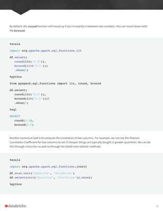
We will start with the last task as it’s one of the simplest. The initcap function will capitalize every word in a given
string when that word is separated from another via whitespace.
%scala
import org.apache.spark.sql.functions.{initcap}
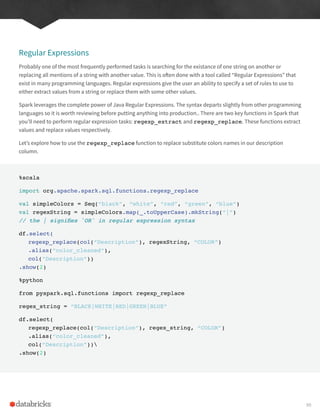
df.select(initcap(col(“Description”))).show(2, false)
%python
from pyspark.sql.functions import initcap
df.select(initcap(col(“Description”))).show()
%sql
SELECT
initcap(Description)
FROM
dfTable
As mentioned above, we can also quite simply lower case and upper case strings as well.
96

97. %scala
import org.apache.spark.sql.functions.{lower, upper}
df.select(
col(“Description”),
lower(col(“Description”)),
upper(lower(col(“Description”))))
.show(2)
%python
from pyspark.sql.functions import lower, upper
df.select(
col(“Description”),
lower(col(“Description”)),
upper(lower(col(“Description”))))
.show(2)
%sql
SELECT
Description,
lower(Description),
Upper(lower(Description))
FROM
dfTable
Another trivial task is adding or removing whitespace around a string. We can do this with lpad, ltrim, rpad and
rtrim, trim.
%scala
import org.apache.spark.sql.functions.{lit, ltrim, rtrim, rpad, lpad, trim}
df.select(
ltrim(lit(“ HELLO “)).as(“ltrim”),
rtrim(lit(“ HELLO “)).as(“rtrim”),
trim(lit(“ HELLO “)).as(“trim”),
97

98. lpad(lit(“HELLO”), 3, “ “).as(“lp”),
rpad(lit(“HELLO”), 10, “ “).as(“rp”))
.show(2)
%python
from pyspark.sql.functions import lit, ltrim, rtrim, rpad, lpad, trim
df.select(
ltrim(lit(“ HELLO “)).alias(“ltrim”),
rtrim(lit(“ HELLO “)).alias(“rtrim”),
trim(lit(“ HELLO “)).alias(“trim”),
lpad(lit(“HELLO”), 3, “ “).alias(“lp”),
rpad(lit(“HELLO”), 10, “ “).alias(“rp”))
.show(2)
%sql
SELECT
ltrim(‘ HELLLOOOO ‘),
rtrim(‘ HELLLOOOO ‘),
trim(‘ HELLLOOOO ‘),
lpad(‘HELLOOOO ‘, 3, ‘ ‘),
rpad(‘HELLOOOO ‘, 10, ‘ ‘)
FROM
dfTable
1trim trim rtrim 1p rp
HELLO
HELLO
HELLO
HELLO
HELLO
HELLO
HE
HE
HELLO
HELLO
only showing top 2 rows
You’ll notice that if lpad or rpad takes a number less than the length of the string, it will always remove values from
the right side of the string.
98

99. Regular Expressions
Probably one of the most frequently performed tasks is searching for the existance of one string on another or
replacing all mentions of a string with another value. This is often done with a tool called “Regular Expressions” that
exist in many programming languages. Regular expressions give the user an ability to specify a set of rules to use to
either extract values from a string or replace them with some other values.
Spark leverages the complete power of Java Regular Expressions. The syntax departs slightly from other programming
languages so it is worth reviewing before putting anything into production.. There are two key functions in Spark that
you’ll need to perform regular expression tasks: regexp_extract and regexp_replace. These functions extract
values and replace values respectively.
Let’s explore how to use the regexp_replace function to replace substitute colors names in our description
column.
%scala
import org.apache.spark.sql.functions.regexp_replace
val simpleColors = Seq(“black”, “white”, “red”, “green”, “blue”)
val regexString = simpleColors.map(_.toUpperCase).mkString(“|”)
// the | signifies `OR` in regular expression syntax
df.select(
regexp_replace(col(“Description”), regexString, “COLOR”)
.alias(“color_cleaned”),
col(“Description”))
.show(2)
%python
from pyspark.sql.functions import regexp_replace
regex_string = “BLACK|WHITE|RED|GREEN|BLUE”
df.select(
regexp_replace(col(“Description”), regex_string, “COLOR”)
.alias(“color_cleaned”),
col(“Description”))
.show(2)
99

100. %sql
SELECT
regexp_replace(Description, ‘BLACK|WHITE|RED|GREEN|BLUE’, ‘COLOR’) as
color_cleaned,
Description
FROM
dfTable
color_cleaned Description
COLOR HANGING HEA...
COLOR METAL LANTERN
WHITE HANGING HEA...
WHITE METAL LANTERN
Another task may be to replace given characters with other characters. Building this as regular expression could be
tedious so Spark also provides the translate function to replace these values. This is done at the character level and
will replace all instances of a character with the indexed character in the replacement string.
%scala
import org.apache.spark.sql.functions.translate
df.select(
translate(col(“Description”), “LEET”, “1337”),
col(“Description”))
.show(2)
%python
from pyspark.sql.functions import translate
df.select(
translate(col(“Description”), “LEET”, “1337”),
col(“Description”))
.show(2)
%sql
100

101. SELECT
translate(Description, ‘LEET’, ‘1337’),
Description
FROM
dfTable
translate(Description, LEET, 1337)| Description
WHI73 HANGING H3A...
WHI73 M37A1 1AN73RN
WHITE HANGING HEA...
WHITE METAL LANTERN
We can also perform something similar like pulling out the first mentioned color.
%scala
import org.apache.spark.sql.functions.regexp_extract
val regexString = simpleColors
.map(_.toUpperCase)
.mkString(“(“, “|”, “)”)
// the | signifies OR in regular expression syntax
df.select(
regexp_extract(col(“Description”), regexString, 1)
.alias(“color_cleaned”),
col(“Description”))
.show(2)
%python
from pyspark.sql.functions import regexp_extract
extract_str = “(BLACK|WHITE|RED|GREEN|BLUE)”
df.select(
regexp_extract(col(“Description”), extract_str, 1)
.alias(“color_cleaned”),
101

102. col(“Description”))
.show(2)
%sql
SELECT
regexp_extract(Description, ‘(BLACK|WHITE|RED|GREEN|BLUE)’, 1),
Description
FROM
dfTable
Sometimes, rather than extracting values, we simply want to check for existence. We can do this with the contains
method on each column. This will return a boolean declaring whether it can find that string in the column’s string.
%scala
val containsBlack = col(“Description”).contains(“BLACK”)
val containsWhite = col(“DESCRIPTION”).contains(“WHITE”)
df.withColumn(“hasSimpleColor”, containsBlack.or(containsWhite))
.filter(“hasSimpleColor”)
.select(“Description”)
.show(3, false)
In Python we can use the instr function.
%python
from pyspark.sql.functions import instr
containsBlack = instr(col(“Description”), “BLACK”) >= 1
containsWhite = instr(col(“Description”), “WHITE”) >= 1
df.withColumn(“hasSimpleColor”, containsBlack | containsWhite)
.filter(“hasSimpleColor”)
.select(“Description”)
.show(3, False)
102

103. %sql
SELECT
Description
FROM
dfTable
WHERE
instr(Description, ‘BLACK’) >= 1 OR
instr(Description, ‘WHITE’) >= 1
Description
WHITE HANGING HEART T-LIGHT HOLDER
WHITE METAL LANTERN
RED WOOLLY HOTTIE WHITE HEART.
only showing top 3 rows
This is trivial with just two values but gets much more complicated with more values.
Let’s work through this in a more dynamic way and take advantage of Spark’s ability to accept a dynamic number
of arguments. When we convert a list of values into a set of arguments and pass them into a function, we use a
language feature called varargs. This feature allows us to effectively unravel an array of arbitrary length and pass it as
arguments to a function. This, coupled with select allows us to create arbitrary numbers of columns dynamically.
%scala
val simpleColors = Seq(“black”, “white”, “red”, “green”, “blue”)
val selectedColumns = simpleColors.map(color => {
col(“Description”)
.contains(color.toUpperCase)
.alias(s”is_$color”)
}):+expr(“*”) // could also append this value
103

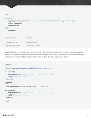
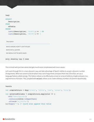
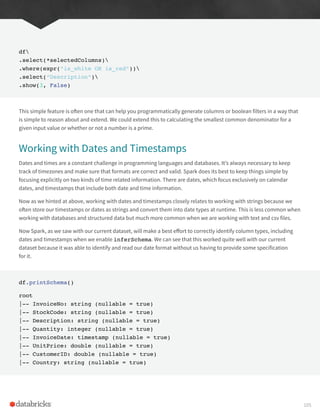
104. df
.select(selectedColumns:_*)
.where(col(“is_white”).or(col(“is_red”)))
.select(“Description”)
.show(3, false)
Description
WHITE HANGING HEART T-LIGHT HOLDER
WHITE METAL LANTERN
RED WOOLLY HOTTIE WHITE HEART.
We can also do this quite easily in Python. In this case we’re going to use a different function locate that returns the
integer location (1 based location). We then convert that to a boolean before using it as a the same basic feature.
%python
from pyspark.sql.functions import expr, locate
simpleColors = [“black”, “white”, “red”, “green”, “blue”]
def color_locator(column, color_string):
“””This function creates a column declaring whether or
not a given pySpark column contains the UPPERCASED
color.
Returns a new column type that can be used
in a select statement.
“””
return locate(color_string.upper(), column)
.cast(“boolean”)
.alias(“is_” + c)
selectedColumns = [color_locator(df.Description, c) for c in simpleColors]
selectedColumns.append(expr(“*”)) # has to a be Column type
104

105. df
.select(*selectedColumns)
.where(expr(“is_white OR is_red”))
.select(“Description”)
.show(3, False)
This simple feature is often one that can help you programmatically generate columns or boolean filters in a way that
is simple to reason about and extend. We could extend this to calculating the smallest common denominator for a
given input value or whether or not a number is a prime.
Working with Dates and Timestamps
Dates and times are a constant challenge in programming languages and databases. It’s always necessary to keep
track of timezones and make sure that formats are correct and valid. Spark does its best to keep things simple by
focusing explicitly on two kinds of time related information. There are dates, which focus exclusively on calendar
dates, and timestamps that include both date and time information.
Now as we hinted at above, working with dates and timestamps closely relates to working with strings because we
often store our timestamps or dates as strings and convert them into date types at runtime. This is less common when
working with databases and structured data but much more common when we are working with text and csv files.
Now Spark, as we saw with our current dataset, will make a best effort to correctly identify column types, including
dates and timestamps when we enable inferSchema. We can see that this worked quite well with our current
dataset because it was able to identify and read our date format without us having to provide some specification
for it.
df.printSchema()
root
|-- InvoiceNo: string (nullable = true)
|-- StockCode: string (nullable = true)
|-- Description: string (nullable = true)
|-- Quantity: integer (nullable = true)
|-- InvoiceDate: timestamp (nullable = true)
|-- UnitPrice: double (nullable = true)
|-- CustomerID: double (nullable = true)
|-- Country: string (nullable = true)
105

106. While Spark will do this on a best effort basis, sometimes there will be no getting around working with strangely
formatted dates and times. Now the key to reasoning about the transformations that you are going to need to apply
is to ensure that you know exactly what type and format you have at each given step of the way. Another common
gotcha is that Spark’s TimestampType only supports second-level precision, this means that if you’re going to
be working with milliseconds or microseconds, you’re going to have to work around this problem by potentially
operating on them as longs. Any more precision when coercing to a TimestampType will be removed.
Spark can be a bit particular about what format you have at any given point in time. It’s important to be explicit when
parsing or converting to make sure there are no issues in doing so. At the end of the day, Spark is working with Java
dates and timestamps and therefore conforms to those standards. Let’s start with the basics and get the current date
and the current timestamps.
%scala
import org.apache.spark.sql.functions.{current_date, current_timestamp}
val dateDF = spark.range(10)
.withColumn(“today”, current_date())
.withColumn(“now”, current_timestamp())
dateDF.createOrReplaceTempView(“dateTable”)
%python
from pyspark.sql.functions import current_date, current_timestamp
dateDF = spark.range(10)
.withColumn(“today”, current_date())
.withColumn(“now”, current_timestamp())
dateDF.createOrReplaceTempView(“dateTable”)
dateDF.printSchema()
Now that we have a simple DataFrame to work with, let’s add and subtract 5 days from today. These functions take a
column and then the number of days to either add or subtract as the arguments.
%scala
import org.apache.spark.sql.functions.{date_add, date_sub}
106

107. dateDF
.select(
date_sub(col(“today”), 5),
date_add(col(“today”), 5))
.show(1)
%python
from pyspark.sql.functions import date_add, date_sub
dateDF
.select(
date_sub(col(“today”), 5),
date_add(col(“today”), 5))
.show(1)
%sql
SELECT
date_sub(today, 5),
date_add(today, 5)
FROM
dateTable
Another common task is to take a look at the difference between two dates. We can do this with the datediff
function that will return the number of days in between two dates. Most often we just care about the days although
since months can have a strange number of days there also exists a function months_between that gives you the
number of months between two dates.
%scala
import org.apache.spark.sql.functions.{datediff, months_between, to_date}
dateDF
.withColumn(“week_ago”, date_sub(col(“today”), 7))
.select(datediff(col(“week_ago”), col(“today”)))
.show(1)
dateDF
.select(
107

108. to_date(lit(“2016-01-01”)).alias(“start”),
to_date(lit(“2017-05-22”)).alias(“end”))
.select(months_between(col(“start”), col(“end”)))
.show(1)
%python
from pyspark.sql.functions import datediff, months_between, to_date
dateDF
.withColumn(“week_ago”, date_sub(col(“today”), 7))
.select(datediff(col(“week_ago”), col(“today”)))
.show(1)
dateDF
.select(
to_date(lit(“2016-01-01”)).alias(“start”),
to_date(lit(“2017-05-22”)).alias(“end”))
.select(months_between(col(“start”), col(“end”)))
.show(1)
%sql
SELECT
to_date(‘2016-01-01’),
months_between(‘2016-01-01’, ‘2017-01-01’),
datediff(‘2016-01-01’, ‘2017-01-01’)
FROM
dateTable
You’ll notice that I introduced a new function above, the to_date function. This function allows us to convert a date
of the format “2017-01-01” to a Spark date. Of course, for this to work our date must be in the year-month-day
format. You’ll notice that in order to perform this I’m also using the lit function which ensures that we’re returning a
literal value in our expression not trying to evaluate subtraction.
%scala
import org.apache.spark.sql.functions.{to_date, lit}
108

109. spark.range(5).withColumn(“date”, lit(“2017-01-01”))
.select(to_date(col(“date”)))
.show(1)
%python
from pyspark.sql.functions import to_date, lit
spark.range(5).withColumn(“date”, lit(“2017-01-01”))
.select(to_date(col(“date”)))
.show(1)
WARNING
Spark will not throw an error if it cannot parse the date, it’ll just return null. This can be a bit tricky in larger
pipelines because you may be expecting your data in one format and getting it in another. To illustrate, let’s take
a look at the date format that has switched from year-month-day to year-day-month. Spark will fail to parse this
date and silently return null instead.
dateDF.select(to_date(lit(“2016-20-12”)),to_date(lit(“2017-12-11”))).show(1)
to_date(2016-20-12) to_date(2017-12-11)
null 2017-12-11
We find this to be an especially tricky situation for bugs because some dates may match the correct format while
others do not. See how above, the second date is show to be Decembers 11th instead of the correct day, November
12th? Spark doesn’t throw an error because it cannot know whether the days are mixed up or if that specific row is
incorrect.
Let’s fix this pipeline, step by step and come up with a robust way to avoid these issues entirely. The first step is
to remember that we need to specify our date format according to the Java SimpleDateFormat standard as
documented in https: //docs.oracle.com/javase/8/docs/api/java/text/SimpleDateFormat.html.
109

110. By using the unix_timestamp we can parse our date into a bigInt that specifies the Unix timestamp in seconds.
We can then cast that to a literal timestamp before passing that into the to_date format which accepts
timestamps, strings, and other dates.
import org.apache.spark.sql.functions.{unix_timestamp, from_unixtime}
val dateFormat = “yyyy-dd-MM”
val cleanDateDF = spark.range(1)
.select(
to_date(unix_timestamp(lit(“2017-12-11”), dateFormat).cast(“timestamp”))
.alias(“date”),
to_date(unix_timestamp(lit(“2017-20-12”), dateFormat).cast(“timestamp”))
.alias(“date2”))
cleanDateDF.createOrReplaceTempView(“dateTable2”)
%python
from pyspark.sql.functions import unix_timestamp, from_unixtime
dateFormat = “yyyy-dd-MM”
cleanDateDF = spark.range(1)
.select(
to_date(unix_timestamp(lit(“2017-12-11”), dateFormat).cast(“timestamp”))
.alias(“date”),
to_date(unix_timestamp(lit(“2017-20-12”), dateFormat).cast(“timestamp”))
.alias(“date2”))
cleanDateDF.createOrReplaceTempView(“dateTable2”)
%sql
SELECT
to_date(cast(unix_timestamp(date, ‘yyyy-dd-MM’) as timestamp)),
to_date(cast(unix_timestamp(date2, ‘yyyy-dd-MM’) as timestamp)),
to_date(date)
FROM
dateTable2
The above example code also shows us how easy it is to cast between timestamps and dates.
110

111. %scala
cleanDateDF
.select(
unix_timestamp(col(“date”), dateFormat).cast(“timestamp”))
.show()
%python
cleanDateDF
.select(
unix_timestamp(col(“date”), dateFormat).cast(“timestamp”))
.show()
Once we’ve gotten our date or timestamp into the correct format and type,Comparing between them is actually quite
easy. We just need to be sure to either use a date/timestamp type or specify our string according to the right format of
yyyy-MM-dd if we’re comparing a date.
cleanDateDF.filter(col(“date2”) > lit(“2017-12-12”)).show()
One minor point is that we can also set this as a string which Spark parses to a literal.
cleanDateDF.filter(col(“date2”) > “’2017-12-12’”).show()
Working with Nulls in Data
As a best practice, you should always use nulls to represent missing or empty data in your DataFrames. Spark can
optimize working with null values more than it can if you use empty strings or other values. The primary way of
interacting with null values, at DataFrame scale, is to use the .na subpackage on a DataFrame.
In Spark there are two things you can do with null values. You can explicitly drop nulls or you can fill them with a value
(globally or on a per column basis).
Let’s experiment with each of these now.
111

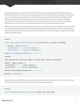
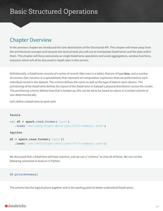
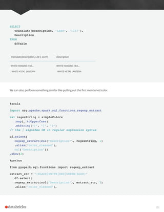
112. Drop
The simplest is probably drop, which simply removes rows that contain nulls. The default is to drop any row where
any value is null.
df.na.drop()
df.na.drop(“any”)
In SQL we have to do this column by column.
%sql
SELECT
*
FROM
dfTable
WHERE
Description IS NOT NULL
Passing in “any” as an argument will drop a row if any of the values are null. Passing in “all” will only drop the row if all
values are null or NaN for that row.
df.na.drop(“all”)
We can also apply this to certain sets of columns by passing in an array of columns.
%scala
df.na.drop(“all”, Seq(“StockCode”, “InvoiceNo”))
%python
df.na.drop(“all”, subset=[“StockCode”, “InvoiceNo”])
112

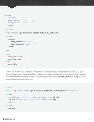
113. Fill
Fill allows you to fill one or more columns with a set of values. This can be done by specifying a map, specific value
and a set of columns.
For example to fill all null values in String columns I might specify.
df.na.fill(“All Null values become this string”)
We could do the same for integer columns with df.na.fill(5:Integer) or for Doubles df.na.
fill(5:Double). In order to specify columns, we just pass in an array of column names like we did above.
%scala
df.na.fill(5, Seq(“StockCode”, “InvoiceNo”))
%python
df.na.fill(“all”, subset=[“StockCode”, “InvoiceNo”])
We can also do with with a Scala Map where the key is the column name and the value is the value we would like to
use to fill null values.
%scala
val fillColValues = Map(
“StockCode” -> 5,
“Description” -> “No Value”
)
df.na.fill(fillColValues)
%python
113

114. fill_cols_vals = {
“StockCode”: 5,
“Description” : “No Value”
}
df.na.fill(fill_cols_vals)
Replace
In addition to replacing null values like we did with drop and fill, there are more flexible options that we can use
with more than just null values. Probably the most common use case is to replace all values in a certain column
according to their current value. The only requirement is that this value be the same type as the original value.
%scala
df.na.replace(“Description”, Map(“” -> “UNKNOWN”))
%python
df.na.replace([“”], [“UNKNOWN”], “Description”)
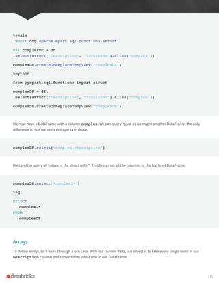
Working with Complex Types
Complex types can help you organize and structure your data in ways that make more sense for the problem you are
hoping to solve. There are three kinds of complex types, structs, arrays, and maps.
Structs
You can think of structs as DataFrames within DataFrames. A worked example will illustrate this more clearly. We can
create a struct by wrapping a set of columns in parenthesis in a query.
df.selectExpr(“(Description, InvoiceNo) as complex”, “*”)
df.selectExpr(“struct(Description, InvoiceNo) as complex”, “*”)
114

115. %scala
import org.apache.spark.sql.functions.struct
val complexDF = df
.select(struct(“Description”, “InvoiceNo”).alias(“complex”))
complexDF.createOrReplaceTempView(“complexDF”)
%python
from pyspark.sql.functions import struct
complexDF = df
.select(struct(“Description”, “InvoiceNo”).alias(“complex”))
complexDF.createOrReplaceTempView(“complexDF”)
We now have a DataFrame with a column complex. We can query it just as we might another DataFrame, the only
difference is that we use a dot syntax to do so.
complexDF.select(“complex.Description”)
We can also query all values in the struct with *. This brings up all the columns to the top level DataFrame.
complexDF.select(“complex.*”)
%sql
SELECT
complex.*
FROM
complexDF
Arrays
To define arrays, let’s work through a use case. With our current data, our object is to take every single word in our
Description column and convert that into a row in our DataFrame.
115

116. The first task is to turn our Description column into a complex type, an array.
split
We do this with the split function and specify the delimiter.
%scala
import org.apache.spark.sql.functions.split
df.select(split(col(“Description”), “ “)).show(2)
%python
from pyspark.sql.functions import split
df.select(split(col(“Description”), “ “)).show(2)
%sql
SELECT
split(Description, ‘ ‘)
FROM
dfTable
This is quite powerful because Spark will allow us to manipulate this complex type as another column. We can also
query the values of the array with a python-like syntax.
%scala
df.select(split(col(“Description”), “ “).alias(“array_col”))
.selectExpr(“array_col[0]”)
.show(2)
%python
df.select(split(col(“Description”), “ “).alias(“array_col”))
.selectExpr(“array_col[0]”)
.show(2)
116

117. %sql
SELECT
split(Description, ‘ ‘)[0]
FROM
dfTable
Array Contains
For instance we can see if this array contains a value.
import org.apache.spark.sql.functions.array_contains
df.select(array_contains(split(col(“Description”), “ “), “WHITE”)).show(2)
%python
from pyspark.sql.functions import array_contains
df.select(array_contains(split(col(“Description”), “ “), “WHITE”)).show(2)
%sql
SELECT
array_contains(split(Description, ‘ ‘), ‘WHITE’)
FROM
dfTable
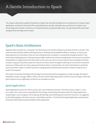
However this does not solve our current problem. In order to convert a complex type into a set of rows (one per value
in our array), we use the explode function.
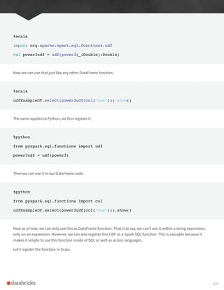
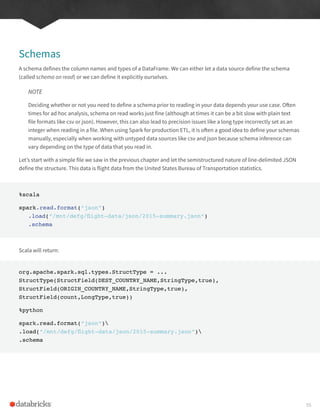
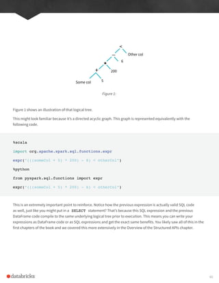
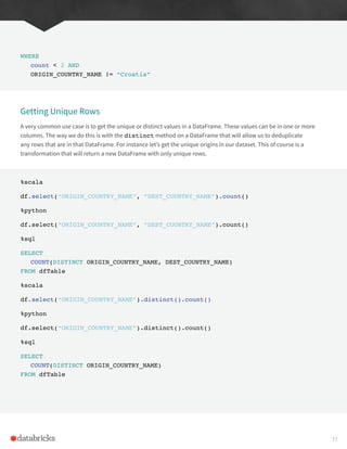
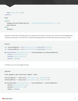
Explode
The explode function takes a column that consists of arrays and creates one row (with the rest of the values
duplicated) per value in the array. The following figure illustrates the process.
117

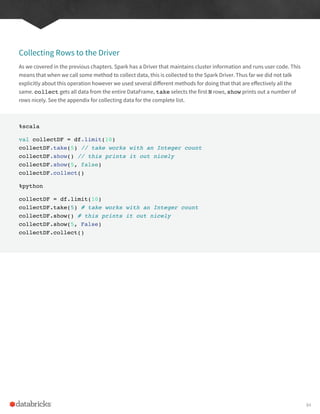
118. %scala
import org.apache.spark.sql.functions.{split, explode}
df.withColumn(“splitted”, split(col(“Description”), “ “))
.withColumn(“exploded”, explode(col(“splitted”)))
.select(“Description”, “InvoiceNo”, “exploded”)
%python
from pyspark.sql.functions import split, explode
df.withColumn(“splitted”, split(col(“Description”), “ “))
.withColumn(“exploded”, explode(col(“splitted”)))
.select(“Description”, “InvoiceNo”, “exploded”)
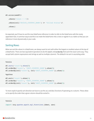
Maps
Maps are used less frequently but are still important to cover. We create them with the map function and key value
pairs of columns. Then we can select them just like we might select from an array.
import org.apache.spark.sql.functions.map
df.select(map(col(“Description”), col(“InvoiceNo”)).alias(“complex_map”))
.selectExpr(“complex_map[‘Description’]”)
Figure 1:
“Hello World” , “other col”
Split Explode
[ “Hello” , “World” ] , “other col” “Hello” , “other col”
“World” , “other col”
118

119. %sql
SELECT
map(Description, InvoiceNo) as complex_map
FROM
dfTable
WHERE
Description IS NOT NULL
We can also explode map types which will turn them into columns.
import org.apache.spark.sql.functions.map
df.select(map(col(“Description”), col(“InvoiceNo”)).alias(“complex_map”))
.selectExpr(“explode(complex_map)”)
.take(5)
Working with JSON
Spark has some unique support for working with JSON data. You can operate directly on strings of JSON in Spark and
parse from JSON or extract JSON objects. Let’s start by creating a JSON column.
%scala
val jsonDF = spark.range(1)
.selectExpr(“””
‘{“myJSONKey” : {“myJSONValue” : [1, 2, 3]}}’ as jsonString
“””)
119

120. %python
jsonDF = spark.range(1)
.selectExpr(“””
‘{“myJSONKey” : {“myJSONValue” : [1, 2, 3]}}’ as jsonString
“””)
We can use the get_json_object to inline query a JSON object, be it a dictionary or array. We can use json_
tuple if this object has only one level of nesting.
%scala
import org.apache.spark.sql.functions.{get_json_object, json_tuple}
jsonDF.select(
get_json_object(col(“jsonString”), “$.myJSONKey.myJSONValue[1]”),
json_tuple(col(“jsonString”), “myJSONKey”))
.show()
%python
from pyspark.sql.functions import get_json_object, json_tuple
jsonDF.select(
get_json_object(col(“jsonString”), “$.myJSONKey.myJSONValue[1]”),
json_tuple(col(“jsonString”), “myJSONKey”))
.show()
The equivalent in SQL would be.
jsonDF.selectExpr(“json_tuple(jsonString, ‘$.myJSONKey.myJSONValue[1]’) as res”)
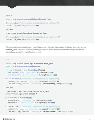
We can also turn a StructType into a JSON string using the to_json function.
120

121. %scala
import org.apache.spark.sql.functions.to_json
df.selectExpr(“(InvoiceNo, Description) as myStruct”)
.select(to_json(col(“myStruct”)))
%python
from pyspark.sql.functions import to_json
df.selectExpr(“(InvoiceNo, Description) as myStruct”)
.select(to_json(col(“myStruct”)))
This function also accepts a dictionary (map) of parameters that are the same as the JSON data source. We can use
the from_json function to parse this (or other json) back in. This naturally requires us to specify a schema and
optionally we can specify a Map of options as well.
%scala
import org.apache.spark.sql.functions.from_json
import org.apache.spark.sql.types._
val parseSchema = new StructType(Array(
new StructField(“InvoiceNo”,StringType,true),
new StructField(“Description”,StringType,true)))
df.selectExpr(“(InvoiceNo, Description) as myStruct”)
.select(to_json(col(“myStruct”)).alias(“newJSON”))
.select(from_json(col(“newJSON”), parseSchema), col(“newJSON”))
%python
from pyspark.sql.functions import from_json
from pyspark.sql.types import *
parseSchema = StructType((
StructField(“InvoiceNo”,StringType(),True),
StructField(“Description”,StringType(),True)))
df.selectExpr(“(InvoiceNo, Description) as myStruct”)
.select(to_json(col(“myStruct”)).alias(“newJSON”))
.select(from_json(col(“newJSON”), parseSchema), col(“newJSON”))
121

122. User-Defined Functions
One of the most powerful things that you can do in Spark is define your own functions. These allow you to write your
own custom transformations using Python or Scala and even leverage external libraries like numpy in doing so. These
functions are called user defined functions or UDFs and can take and return one or more columns as input.
Spark UDFs are incredibly powerful because they can be written in several different programming languages and do
not have to be written in an esoteric format or DSL. They’re just functions that operate on the data, record by record.
While we can write our functions in Scala, Python, or Java, there are performance considerations that you should be
aware of. To illustrate this, we’re going to walk through exactly what happens when you create UDF, pass that into
Spark, and then execute code using that UDF.
The first step is the actual function, we’ll just a take a simple one for this example. We’ll write a power3 function that
takes a number and raises it to a power of three.
%scala
val udfExampleDF = spark.range(5).toDF(“num”)
def power3(number:Double):Double = {
number * number * number
}
power3(2.0)
%python
udfExampleDF = spark.range(5).toDF(“num”)
def power3(double_value):
return double_value ** 3
power3(2.0)
In this trivial example, we can see that our functions work as expected. We are able to provide an individual input and
produce the expected result (with this simple test case). Thus far our expectations for the input are high, it must be a
specific type and cannot be a null value. See the section in this chapter titled “Working with Nulls in Data”.
Now that we’ve created these functions and tested them, we need to register them with Spark so that we can used
them on all of our worker machines. Spark will serialize the function on the driver and transfer it over the network to
all executor processes. This happens regardless of language.
122

123. Once we go to use the function, there are essentially two different things that occur. If the function is written in Scala
or Java then we can use that function within the JVM. This means there will be little performance penalty aside from
the fact that we can’t take advantage of code generation capabilities that Spark has for built-in functions. There can
be performance issues if you create or use a lot of objects which we will cover in the optimization section.
If the function is written in Python, something quite different happens. Spark will start up a python process on the
worker, serialize all of the data to a format that python can understand (remember it was in the JVM before), execute
the function row by row on that data in the python process, before finally returning the results of the row operations
to the JVM and Spark.
WARNING: Starting up this Python process is expensive but the real cost is in serializing the data to Python. This is
costly for two reasons, it is an expensive computation but also once the data enters Python, Spark cannot manage the
memory of the worker. This means that you could potentially cause a worker to fail if it becomes resource constrained
(because both the JVM and python are competing for memory on the same machine). We recommend that you
write your UDFs in Scala - the small amount of time it should take you to write the function in Scala will always yield
significant speed ups and on top of that, you can still use the function from Python!
Now that we have an understanding of the process, let’s work through our example. First we need to register the
function to be available as a DataFrame function.
Figure 2:
Spark Session
Executor processes Worker python process
Scala UDF
Python UDF
1. Function serialized
and sent to workers
3. Python returns
answer
2. Spark starts Python process
and sends data
Driver
123

124. %scala
import org.apache.spark.sql.functions.udf
val power3udf = udf(power3(_:Double):Double)
Now we can use that just like any other DataFrame function.
%scala
udfExampleDF.select(power3udf(col(“num”))).show()
The same applies to Python, we first register it.
%python
from pyspark.sql.functions import udf
power3udf = udf(power3)
Then we can use it in our DataFrame code.
%python
from pyspark.sql.functions import col
udfExampleDF.select(power3udf(col(“num”))).show()
Now as of now, we can only use this as DataFrame function. That is to say, we can’t use it within a string expression,
only on an expression. However, we can also register this UDF as a Spark SQL function. This is valuable because it
makes it simple to use this function inside of SQL as well as across languages.
Let’s register the function in Scala.
124

125. %scala
spark.udf.register(“power3”, power3(_:Double):Double)
udfExampleDF.selectExpr(“power3(num)”).show()
Now because this function is registered with Spark SQL, and we’ve learned that any Spark SQL function or epxression
is valid to use as an expression when working with DataFrames, we can turn around and use the UDF that we wrote in
Scala, in Python. However rather than using it as a DataFrame function we use it as a SQL expression.
%python
udfExampleDF.selectExpr(“power3(num)”).show()
# registered in Scala
We can also register our Python function to be available as SQL function and use that in any language as well.
One thing we can also do to make sure that our functions are working correctly is specify a return type. As we saw in
the beginning of this section, Spark manages its own type information that does not align exactly with Python’s types.
Therefore it’s a best practice to define the return type for your function when you define it. It is important to note that
specifying the return type is not necessary but is a best practice.
If you specify the type that doesn’t align with the actual type returned by the function - Spark will not error but rather
just return null to designate a failure. You can see this if you were to switch the return type in the below function to
be a DoubleType.
%python
from pyspark.sql.types import IntegerType, DoubleType
spark.udf.register(“power3py”, power3, DoubleType())
%python
udfExampleDF.selectExpr(“power3py(num)”).show()
# registered via Python
125

126. This is because the range above creates Integers. When Integers are operated on in Python, Python won’t convert
them into floats (the corresponding type to Spark’s Double type), therefore we see null. We can remedy this by
ensuring our Python function returns a float instead of an Integer and the function will behave correctly.
Naturally we can use either of these from SQL too once we register them.
%sql
SELECT
power3py(12), -- doesn’t work because of return type
power3(12)
This chapter demonstrated how easy it is to extend Spark SQL to your own purposes and do so in a way that is not
some esoteric, domain-specific language but rather simple functions that are easy to test and maintain without even
using Spark! This is an amazingly powerful tool we can use to specify sophisticated business logic that can run on 5
rows on our local machines or on terabytes of data on a hundred node cluster!
126

127. The Unified Analytics Platform
The datasets used in the book are also available for you to explore:
Spark: The Definitive Guide Datasets
Try Databricks for free
databricks.com/try-databricks
Contact us for a personalized demo
databricks.com/contact-databricks
© Databricks 2017. All rights reserved. Apache Spark and the Apache Spark Logo are trademarks of the Apache Software Foundation. 127