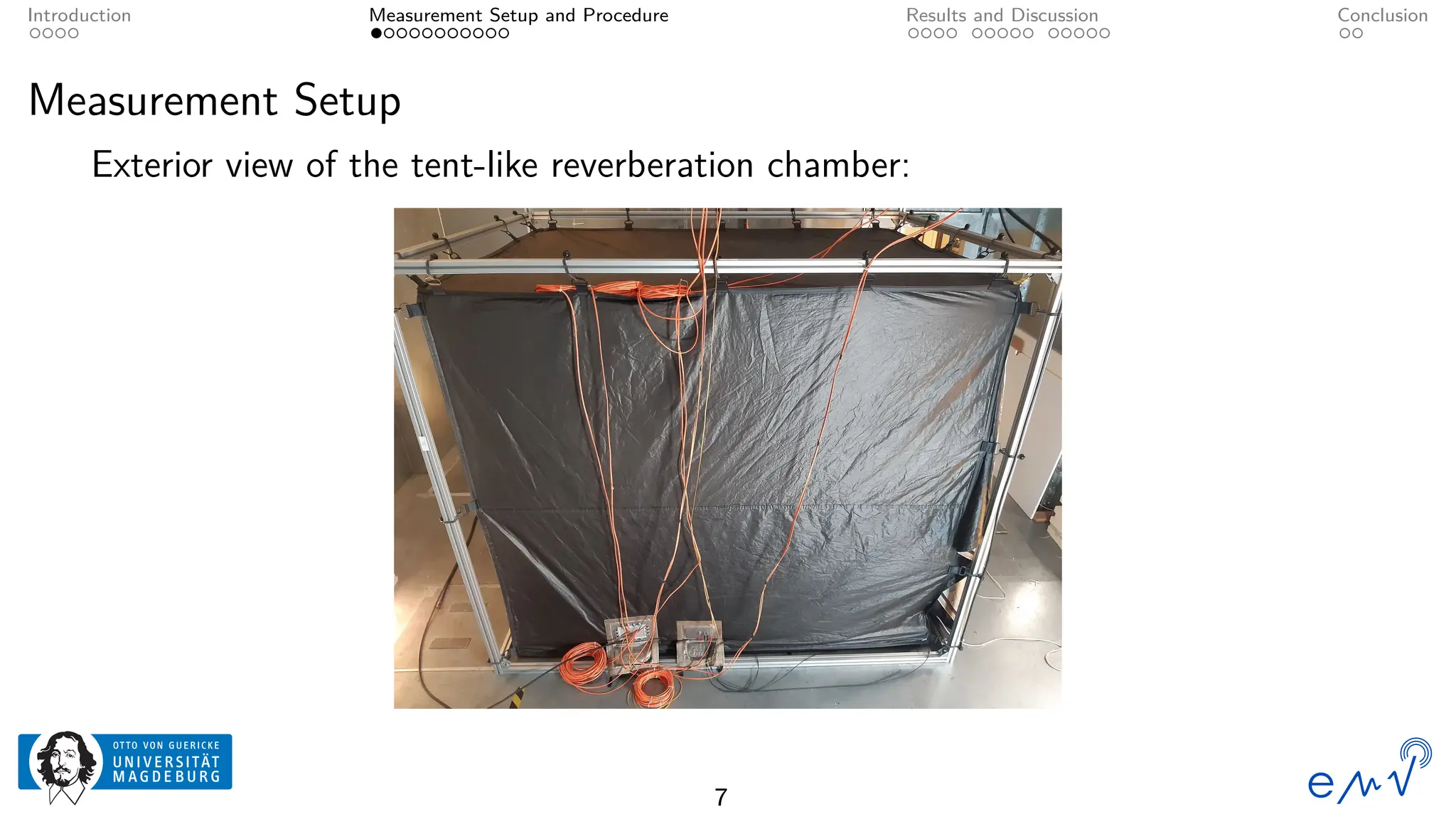
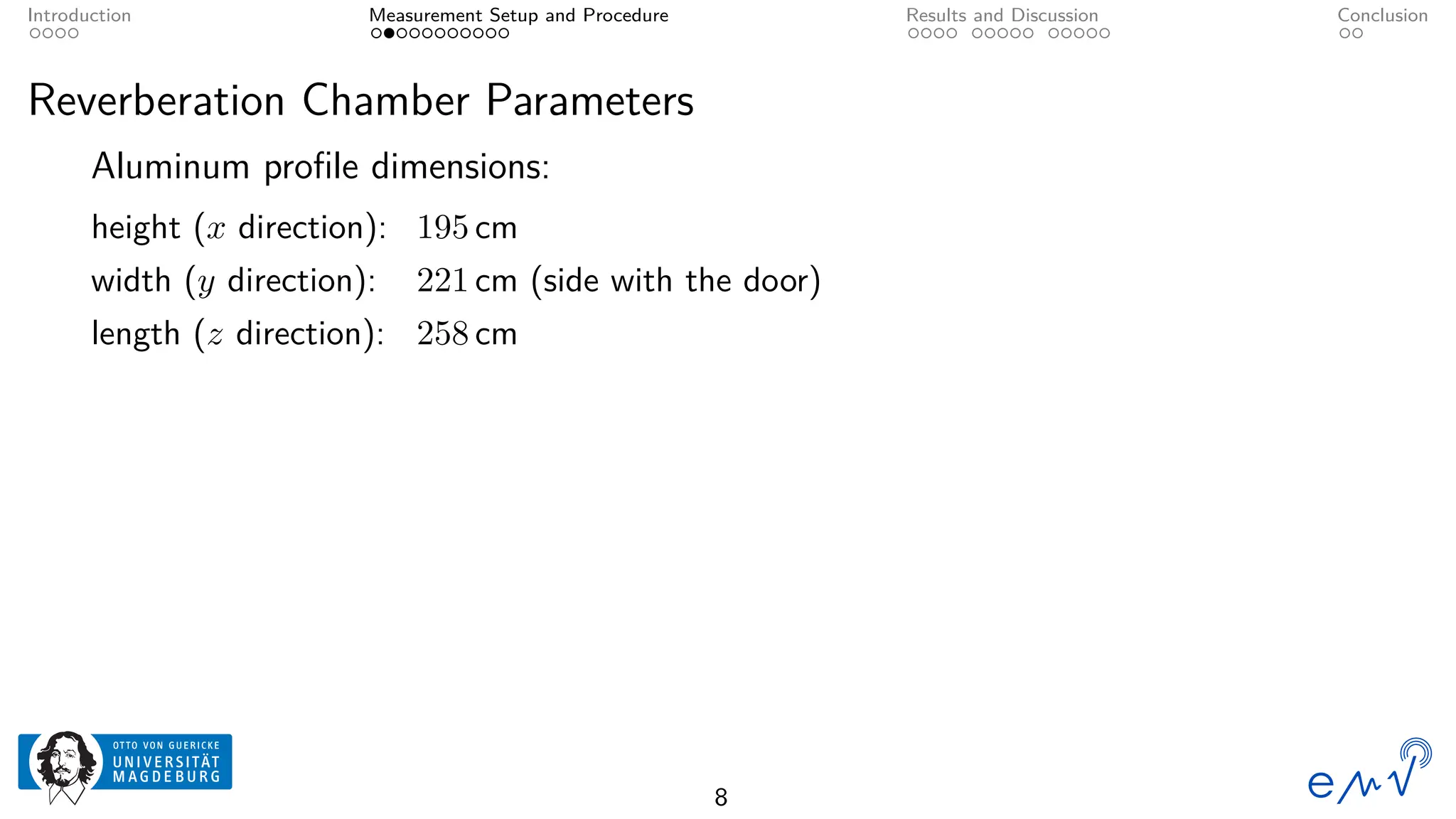
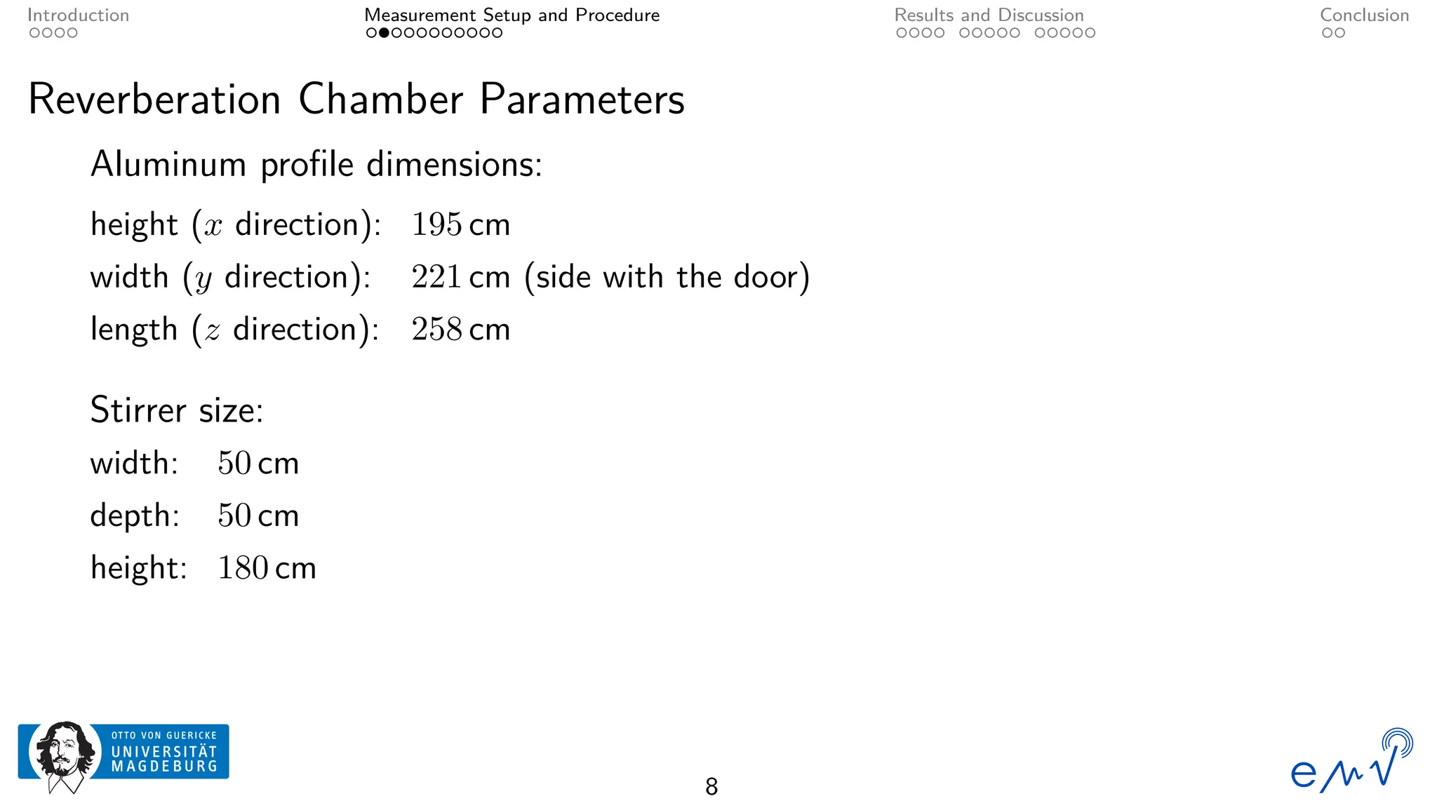
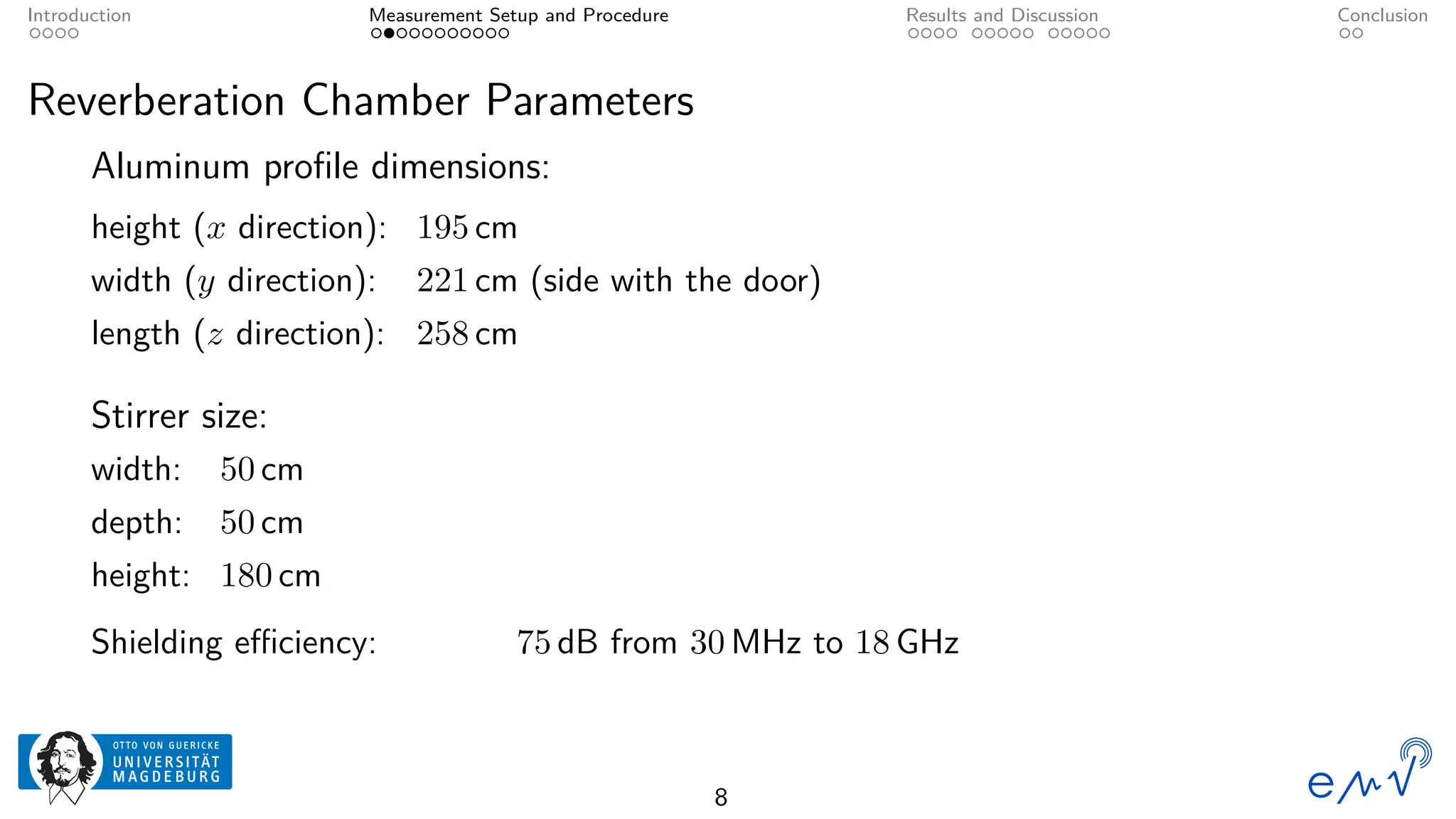
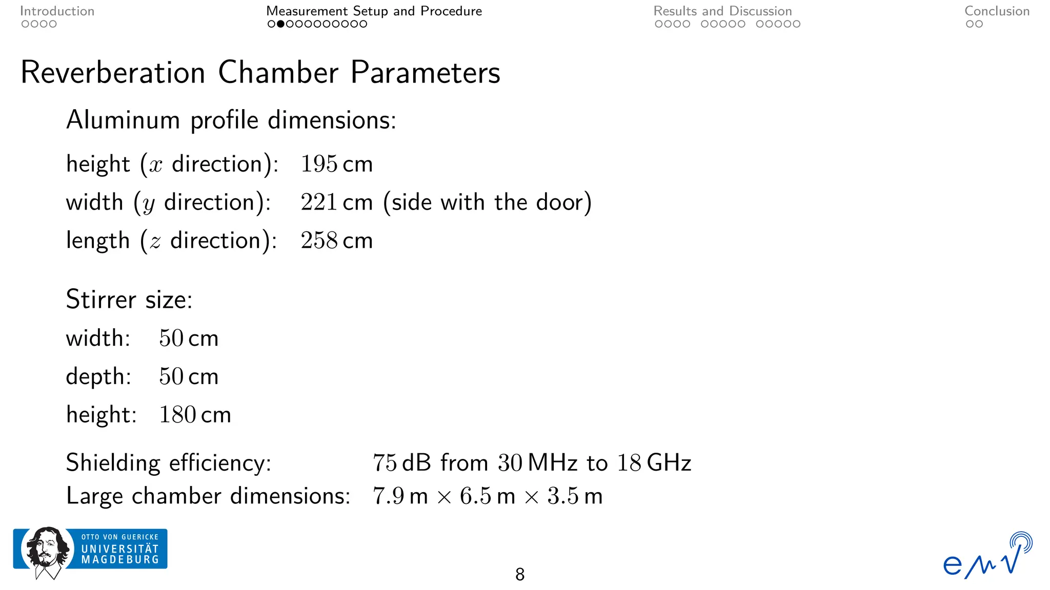
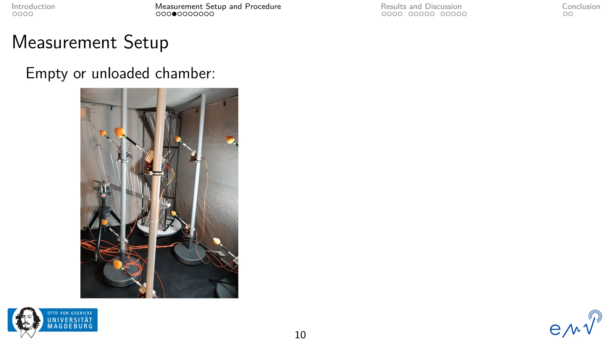
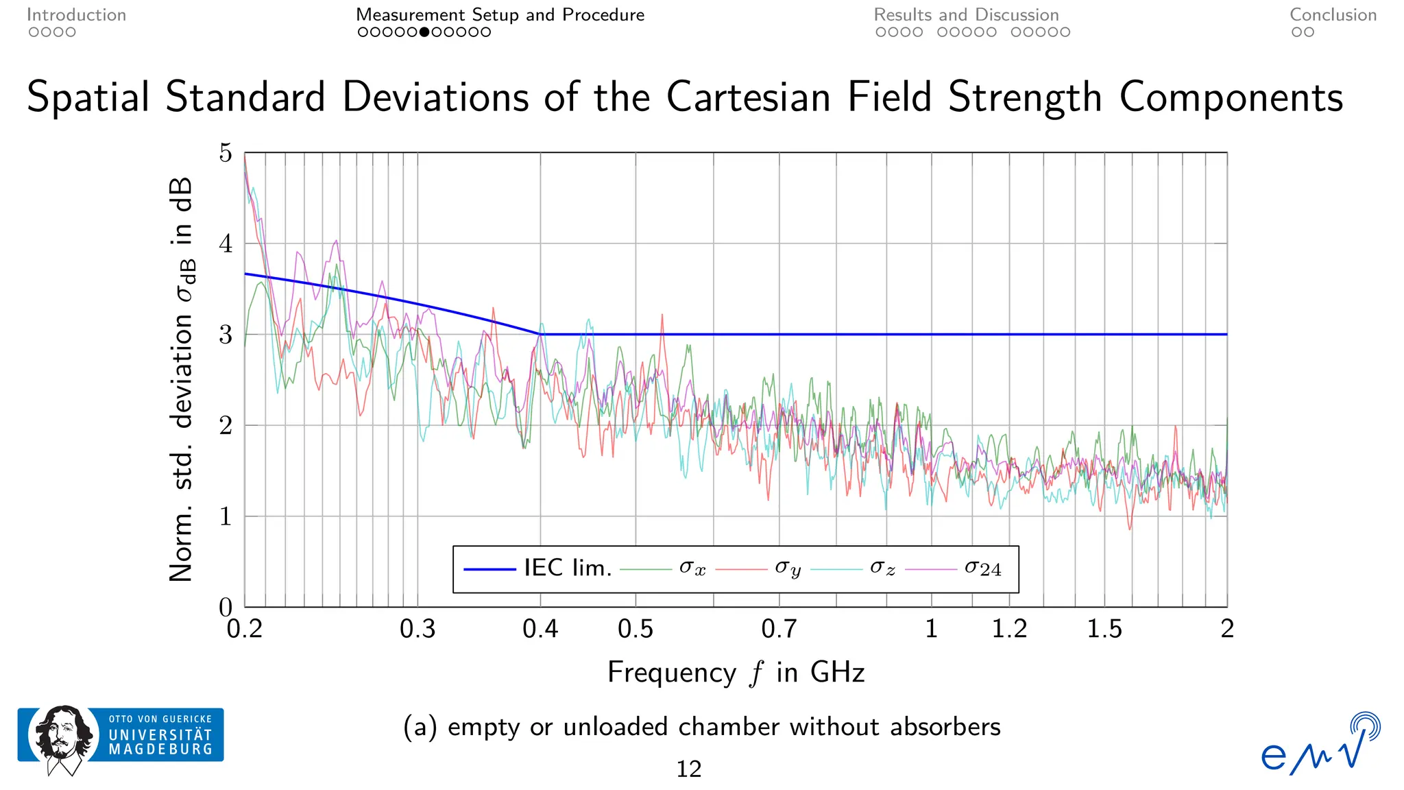
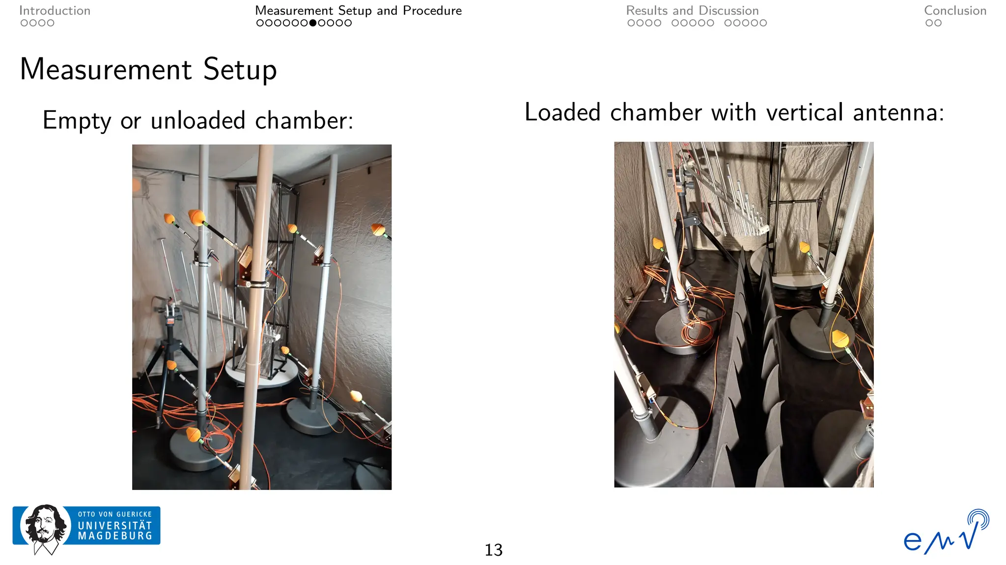
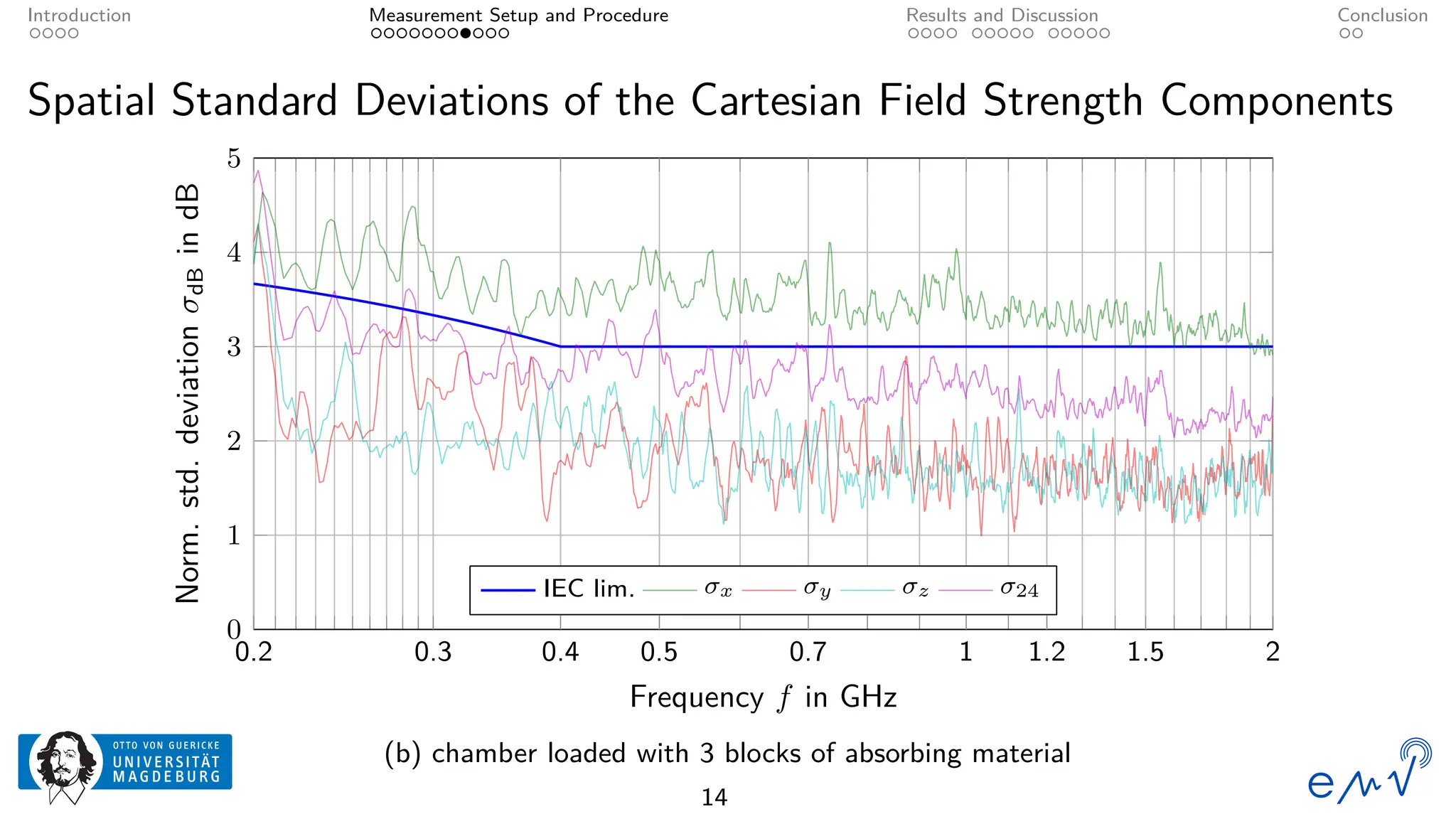
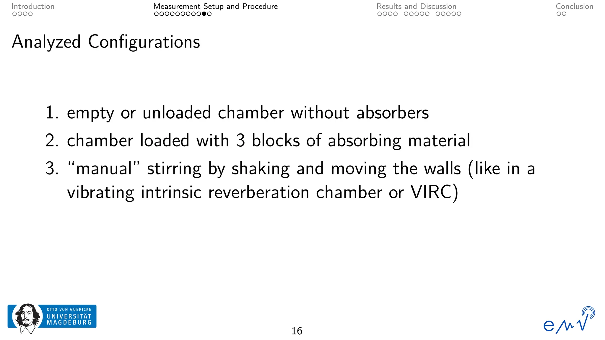
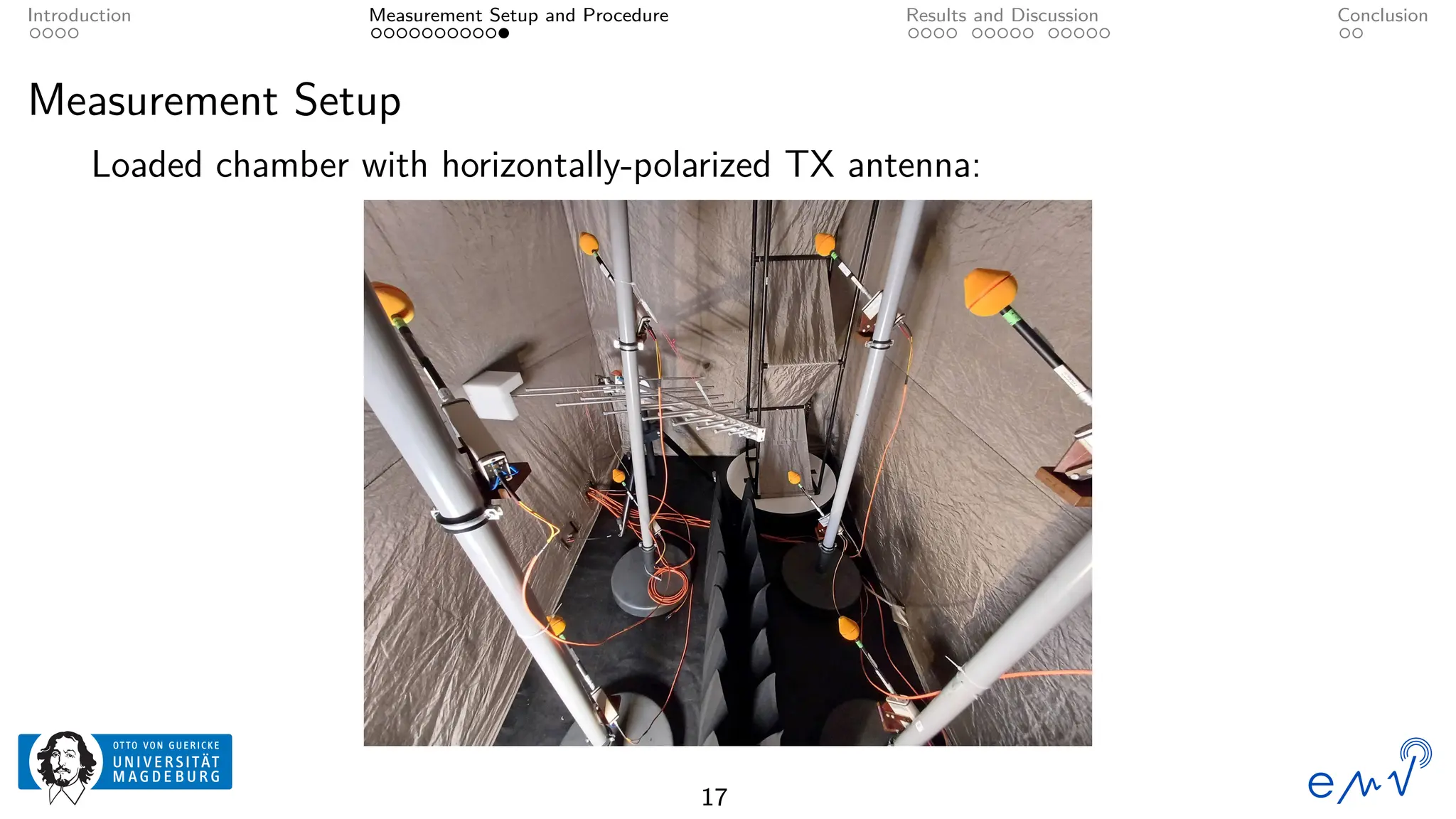
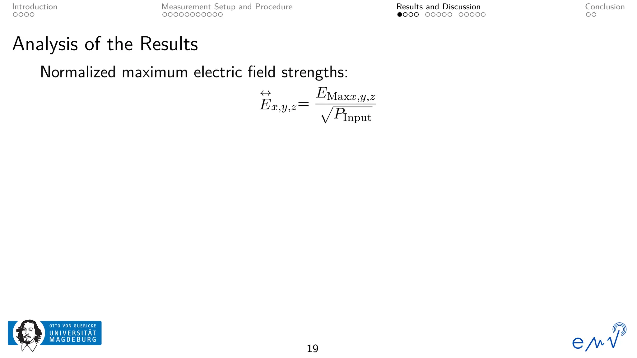
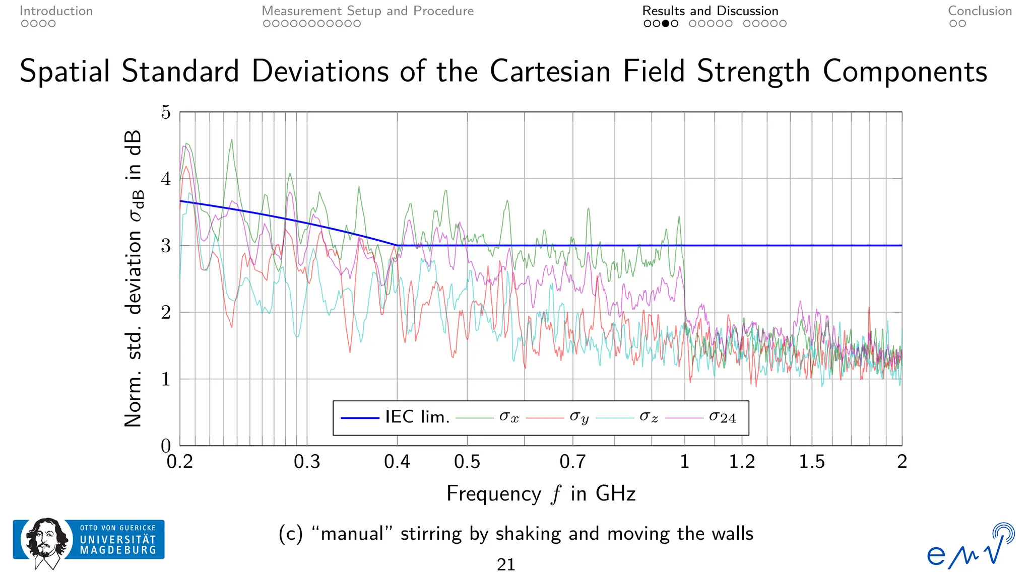
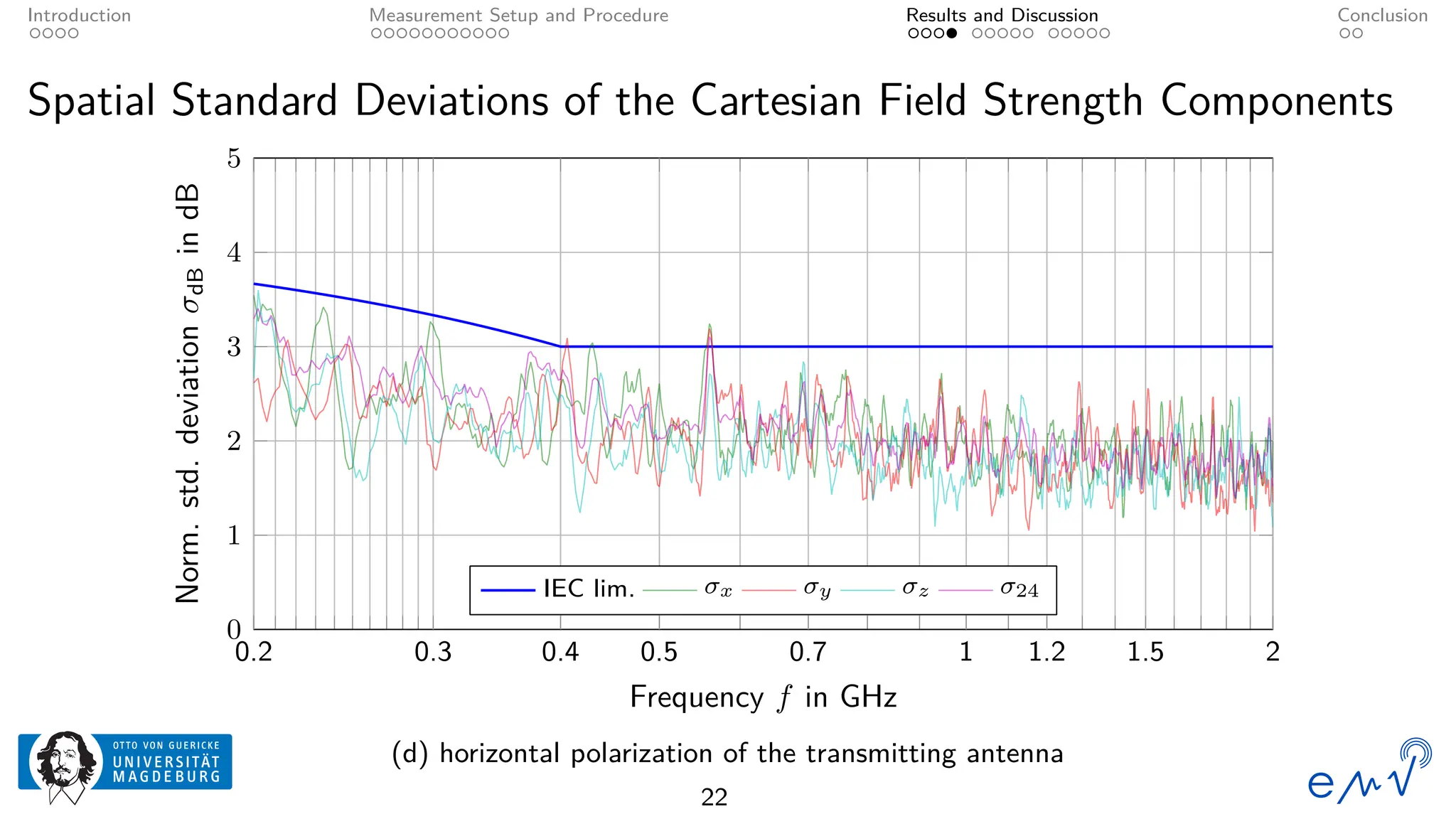
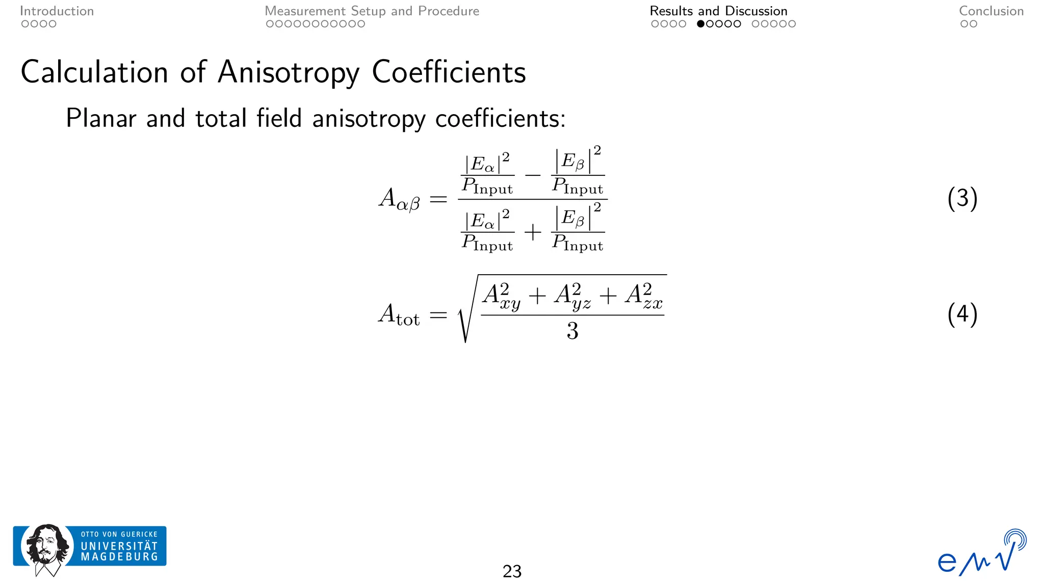
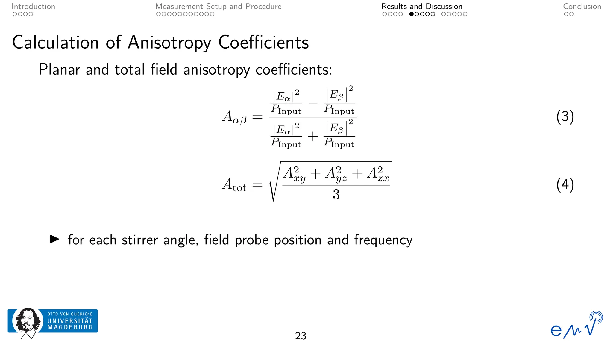
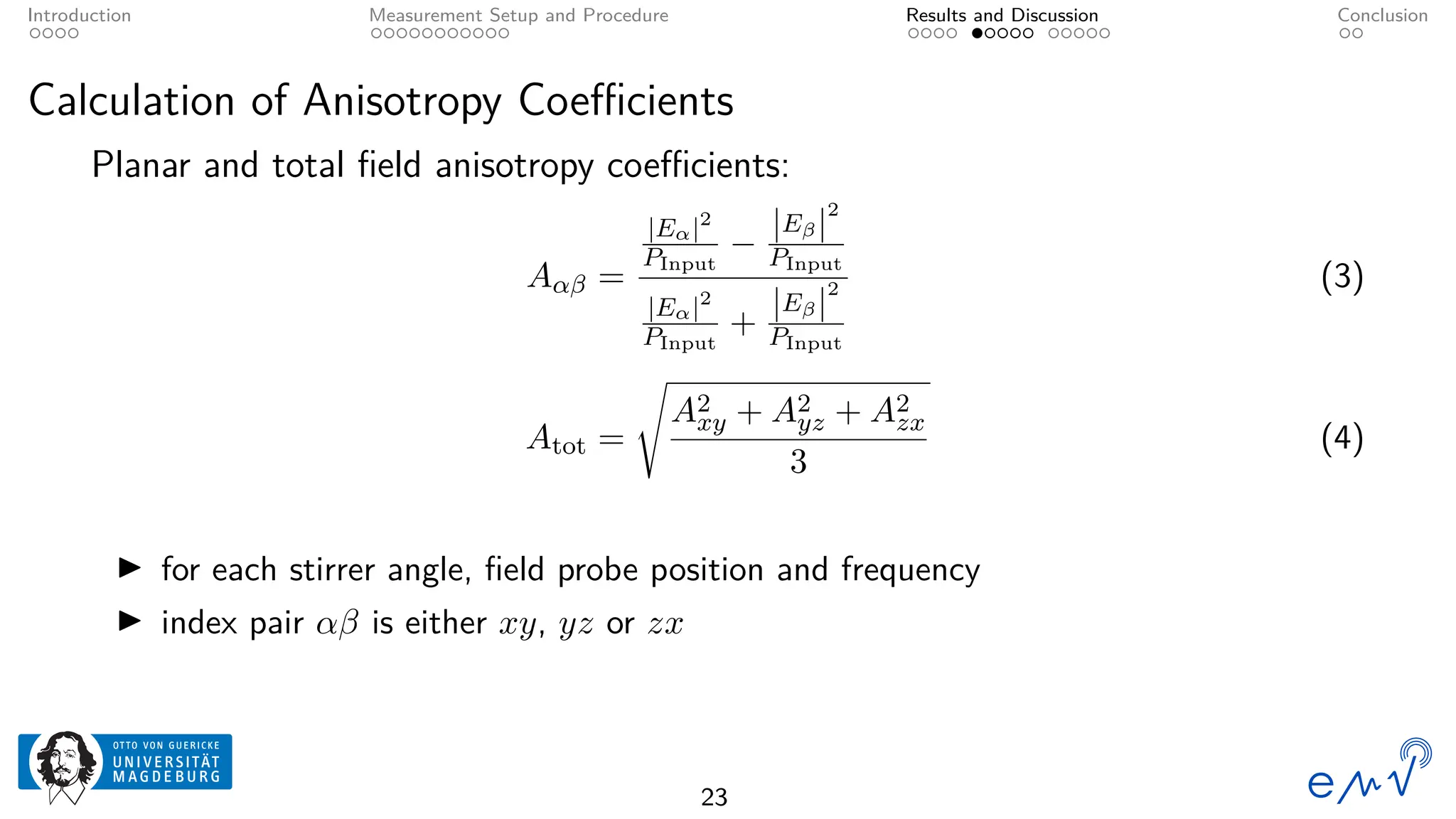
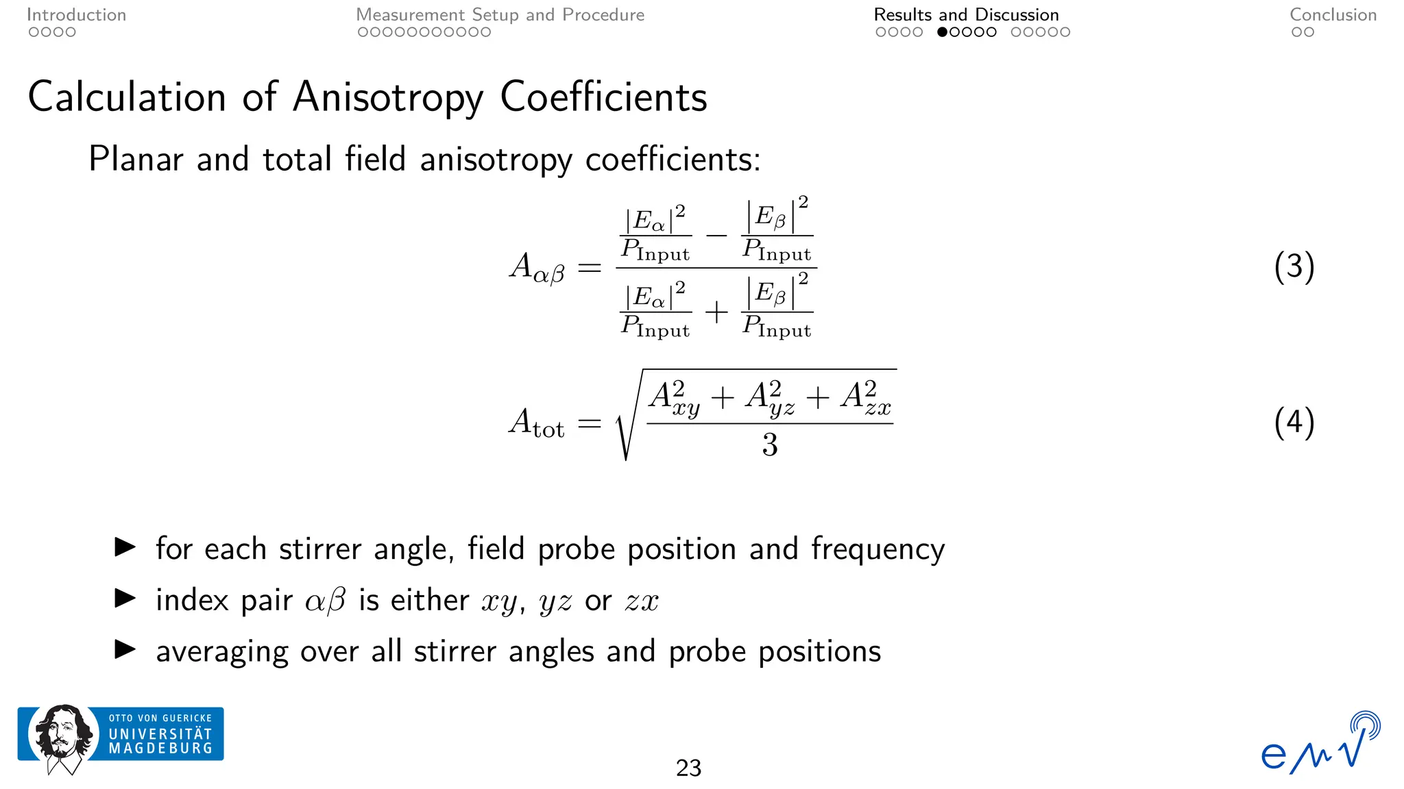
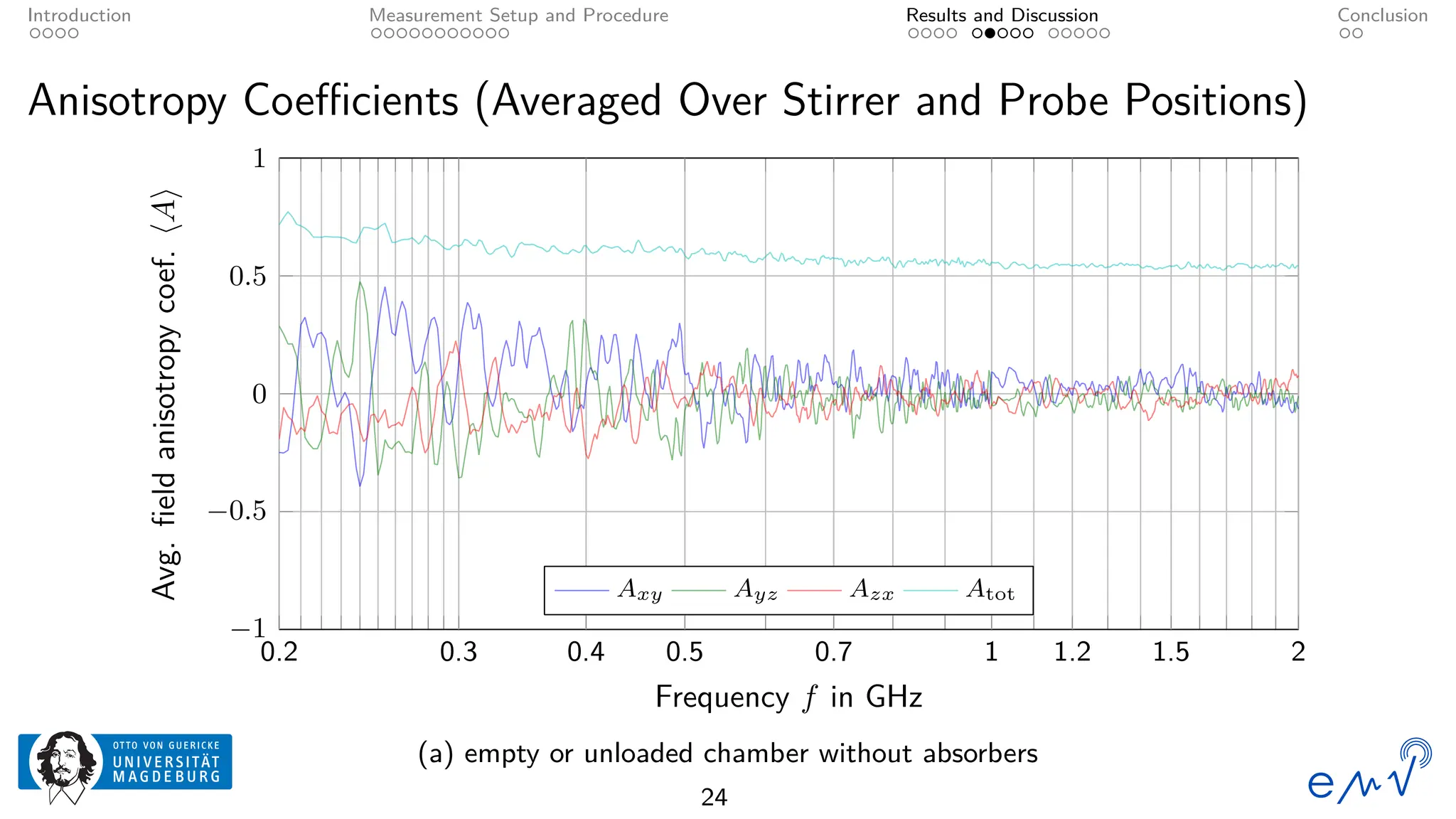
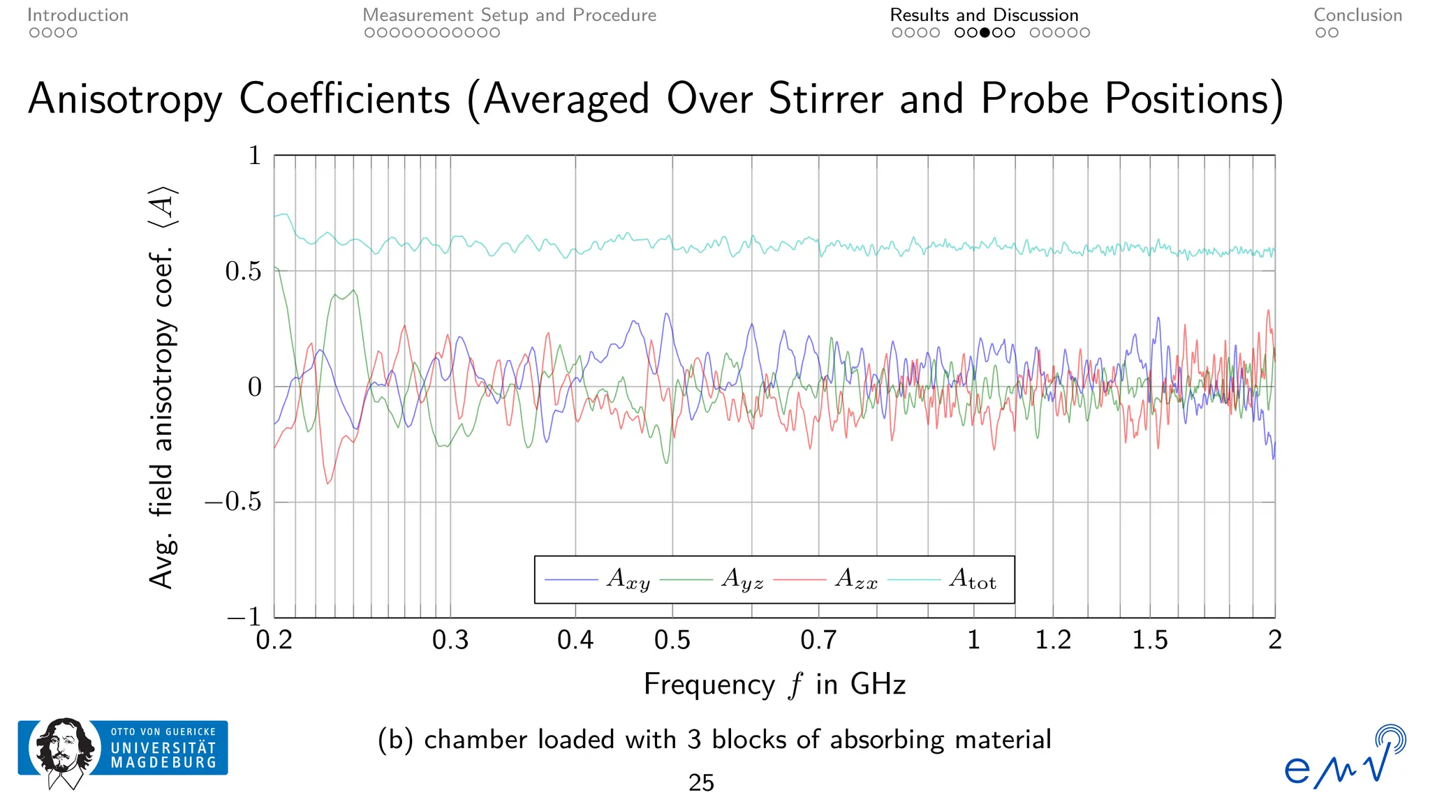
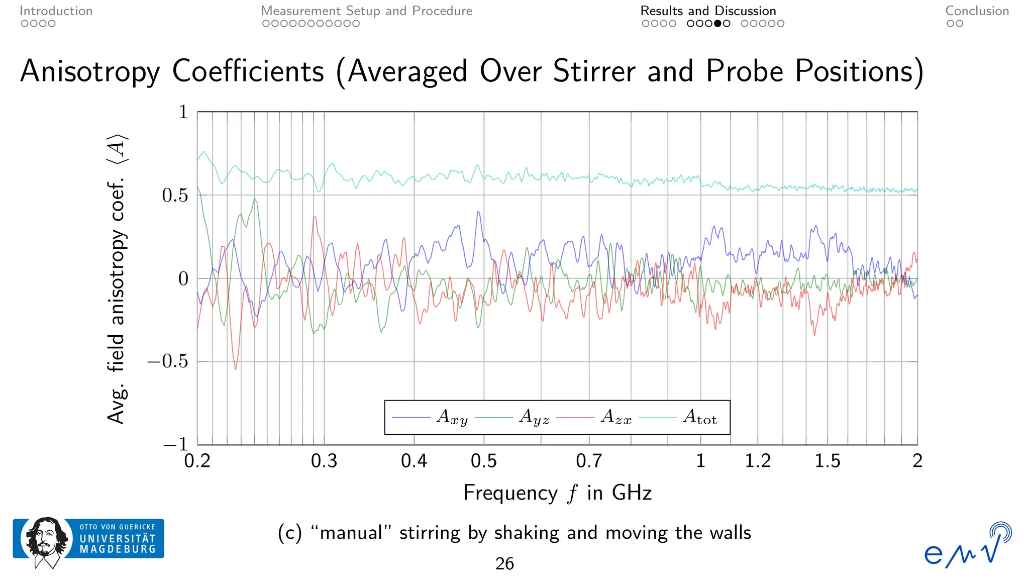
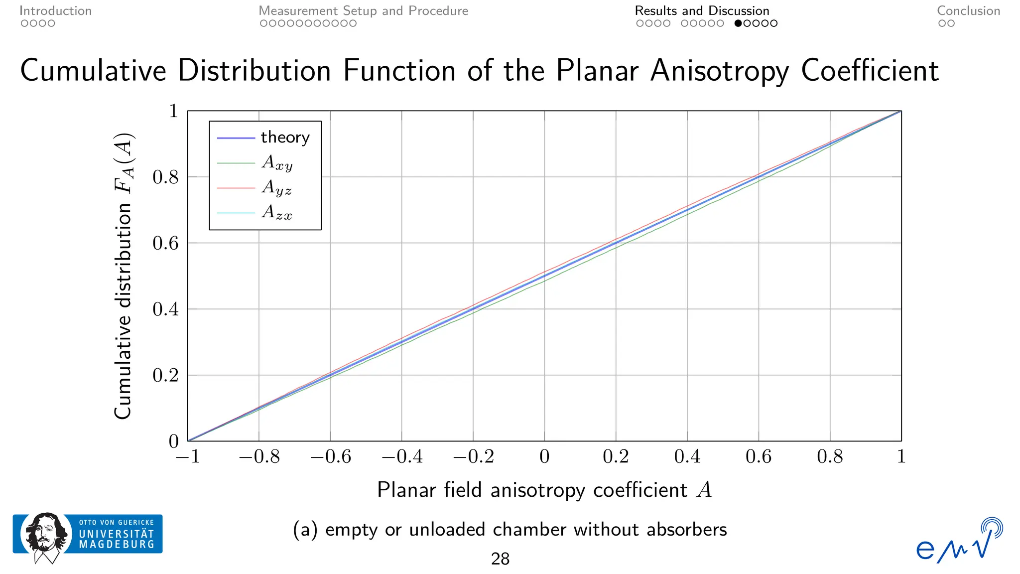
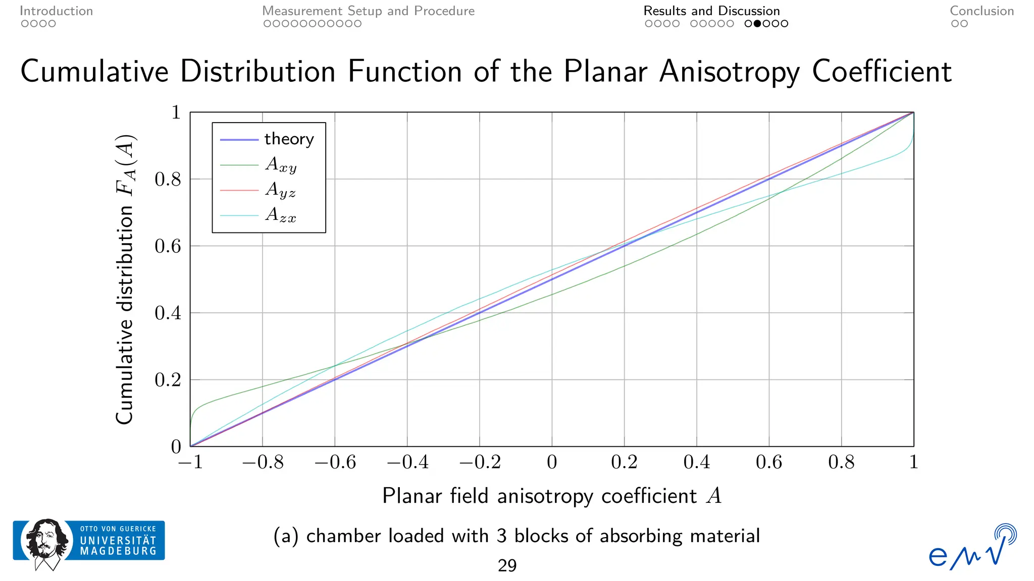
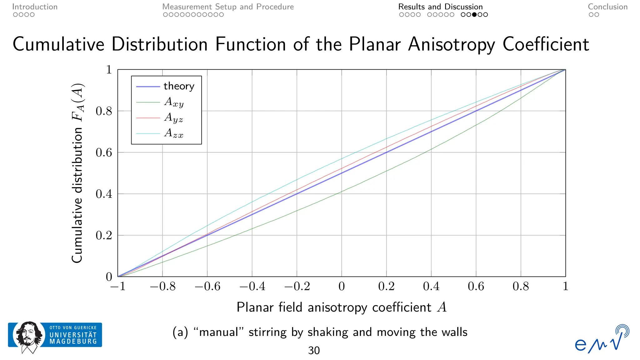
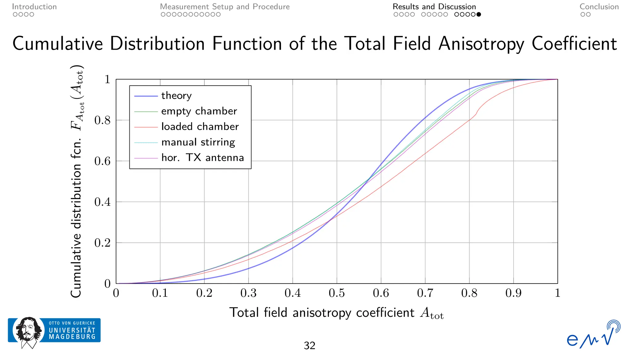
This talk has been given in the session "Measurement Techniques and Test Methods 1" of the ESA Workshop on Aerospace EMC 2025 in Sevilla, Spain. Abstract: The field homogeneity and isotropy of a mobile reverberation chamber made of an aluminum frame and metallized textile has been analyzed for four different configuration, the empty chamber, the chamber loaded with foam absorbers, for manual stirring by shaking the flexible walls and for a different polarization of the transmitting antenna. The measured electrical field strength components have been analyzed according to the standard validation procedure described in Annex B as well as to the planar and total field anisotropy coefficients defined in Annex J of the IEC 61000-4-21. The results show that the loading by anisotropic absorbers in the same orientation as the transmitting antenna drastically affects the field homogeneity, even at frequencies well above the lowest usable frequency. Changing the electromagnetic boundary conditions of the resonant cavity by shaking the walls or rotating the polarization of the transmitting antenna allow for a better homogeneity and isotropy. PDF download: https://cloud.ovgu.de/s/kzEH8znYD3Ya66t

1. Introduction Measurement Setup and Procedure Results and Discussion Conclusion
Analysis of the Field Homogeneity and Isotropy
in a Tent-Like Reverberation Chamber
Mathias Magdowski 1, Sebastian Wessels 2, Ralf Vick 1
(1) Chair for Electromagnetic Compatibility
Institute for Medical Engineering
Faculty of Electrical Engineering and Information Technology
Otto von Guericke University, Magdeburg, Germany
(2) Statex Produktions- und Vertriebs GmbH, Bremen, Germany
May 12, 2025
1

2. Introduction Measurement Setup and Procedure Results and Discussion Conclusion
Some Motivation
2

3. Introduction Measurement Setup and Procedure Results and Discussion Conclusion
Some Motivation
Fast
probes
2

4. Introduction Measurement Setup and Procedure Results and Discussion Conclusion
Some Motivation
Fast
probes
Fast
stirrers
2

5. Introduction Measurement Setup and Procedure Results and Discussion Conclusion
Some Motivation
Fast
probes
Fast
stirrers
Fast
analysis
2

6. Introduction Measurement Setup and Procedure Results and Discussion Conclusion
Some Motivation
Fast
probes
Fast
stirrers
Fast
analysis
PInput Q-factor
Boundary conditions
CDF80%
∆Etarget
PStart
2

7. Introduction Measurement Setup and Procedure Results and Discussion Conclusion
3

8. Introduction Measurement Setup and Procedure Results and Discussion Conclusion
Tent-Like Reverberation Chambers for Flexible Operation
Source: https://imgflip.com/memetemplate/126260959/Tent-on-trailer
4

9. Introduction Measurement Setup and Procedure Results and Discussion Conclusion
Tent-Like Chamber Packet on a Pallet
5

10. Introduction Measurement Setup and Procedure Results and Discussion Conclusion
Overview
Introduction
Measurement Setup and Procedure
Results and Discussion
Spatial Standard Deviations
Anisotropy Coefficients
Cumulative Distribution Functions
Conclusion
6

11. Introduction Measurement Setup and Procedure Results and Discussion Conclusion
Measurement Setup
Exterior view of the tent-like reverberation chamber:
7

12. Introduction Measurement Setup and Procedure Results and Discussion Conclusion
Reverberation Chamber Parameters
Aluminum profile dimensions:
height (x direction): 195 cm
width (y direction): 221 cm (side with the door)
length (z direction): 258 cm
8

13. Introduction Measurement Setup and Procedure Results and Discussion Conclusion
Reverberation Chamber Parameters
Aluminum profile dimensions:
height (x direction): 195 cm
width (y direction): 221 cm (side with the door)
length (z direction): 258 cm
Stirrer size:
width: 50 cm
depth: 50 cm
height: 180 cm
8

14. Introduction Measurement Setup and Procedure Results and Discussion Conclusion
Reverberation Chamber Parameters
Aluminum profile dimensions:
height (x direction): 195 cm
width (y direction): 221 cm (side with the door)
length (z direction): 258 cm
Stirrer size:
width: 50 cm
depth: 50 cm
height: 180 cm
Shielding efficiency: 75 dB from 30 MHz to 18 GHz
8

15. Introduction Measurement Setup and Procedure Results and Discussion Conclusion
Reverberation Chamber Parameters
Aluminum profile dimensions:
height (x direction): 195 cm
width (y direction): 221 cm (side with the door)
length (z direction): 258 cm
Stirrer size:
width: 50 cm
depth: 50 cm
height: 180 cm
Shielding efficiency: 75 dB from 30 MHz to 18 GHz
Large chamber dimensions: 7.9 m × 6.5 m × 3.5 m
8

16. Introduction Measurement Setup and Procedure Results and Discussion Conclusion
Measurement Setup
Schematic of the connection of the instruments:
computer
signal
generator
power
amplifier
adapter
box
motor
controller
optical fiber
LAN
coaxial
cable
GPIB
optical
fiber
9

17. Introduction Measurement Setup and Procedure Results and Discussion Conclusion
Measurement Setup
Empty or unloaded chamber:
10

18. Introduction Measurement Setup and Procedure Results and Discussion Conclusion
Parameters
Settings:
Frequency range: 200 MHz to 2 GHz in steps of 2 MHz to 5 MHz
Expected LUF: around 500 MHz
Input power: 30 dBm to 35 dBm
Stirrer positions: 36 (no automation)
Loop order: frequency sweep for each stirrer position
11

19. Introduction Measurement Setup and Procedure Results and Discussion Conclusion
Spatial Standard Deviations of the Cartesian Field Strength Components
0
1
2
3
4
5
0.2 0.3 0.4 0.5 0.7 1 1.2 1.5 2
Frequency f in GHz
Norm.
std.
deviation
σ
dB
in
dB
IEC lim. σx σy σz σ24
(a) empty or unloaded chamber without absorbers
12

20. Introduction Measurement Setup and Procedure Results and Discussion Conclusion
Measurement Setup
Empty or unloaded chamber: Loaded chamber with vertical antenna:
13

21. Introduction Measurement Setup and Procedure Results and Discussion Conclusion
Spatial Standard Deviations of the Cartesian Field Strength Components
0
1
2
3
4
5
0.2 0.3 0.4 0.5 0.7 1 1.2 1.5 2
Frequency f in GHz
Norm.
std.
deviation
σ
dB
in
dB
IEC lim. σx σy σz σ24
(b) chamber loaded with 3 blocks of absorbing material
14

22. Introduction Measurement Setup and Procedure Results and Discussion Conclusion
15

23. Introduction Measurement Setup and Procedure Results and Discussion Conclusion
Analyzed Configurations
1. empty or unloaded chamber without absorbers
16

24. Introduction Measurement Setup and Procedure Results and Discussion Conclusion
Analyzed Configurations
1. empty or unloaded chamber without absorbers
2. chamber loaded with 3 blocks of absorbing material
16

25. Introduction Measurement Setup and Procedure Results and Discussion Conclusion
Analyzed Configurations
1. empty or unloaded chamber without absorbers
2. chamber loaded with 3 blocks of absorbing material
3. “manual” stirring by shaking and moving the walls (like in a
vibrating intrinsic reverberation chamber or VIRC)
16

26. Introduction Measurement Setup and Procedure Results and Discussion Conclusion
Analyzed Configurations
1. empty or unloaded chamber without absorbers
2. chamber loaded with 3 blocks of absorbing material
3. “manual” stirring by shaking and moving the walls (like in a
vibrating intrinsic reverberation chamber or VIRC)
4. horizontal polarization of the transmitting antenna
16

27. Introduction Measurement Setup and Procedure Results and Discussion Conclusion
Measurement Setup
Loaded chamber with horizontally-polarized TX antenna:
17

28. Introduction Measurement Setup and Procedure Results and Discussion Conclusion
Intermediate Overview
Introduction
Measurement Setup and Procedure
Results and Discussion
Spatial Standard Deviations
Anisotropy Coefficients
Cumulative Distribution Functions
Conclusion
18

29. Introduction Measurement Setup and Procedure Results and Discussion Conclusion
Analysis of the Results
Normalized maximum electric field strengths:
↔
Ex,y,z=
EMaxx,y,z
p
PInput
19

30. Introduction Measurement Setup and Procedure Results and Discussion Conclusion
Analysis of the Results
Normalized maximum electric field strengths:
↔
Ex,y,z=
EMaxx,y,z
p
PInput
Averaging over the eight field probe locations:
D↔
Ex
E
8
=
P8
i=1
↔
Ex,i
8
D↔
Ey
E
8
=
P8
i=1
↔
Ey,i
8
D↔
Ez
E
8
=
P8
i=1
↔
Ez,i
8
19

31. Introduction Measurement Setup and Procedure Results and Discussion Conclusion
Analysis of the Results
Normalized maximum electric field strengths:
↔
Ex,y,z=
EMaxx,y,z
p
PInput
Averaging over the eight field probe locations:
D↔
Ex
E
8
=
P8
i=1
↔
Ex,i
8
D↔
Ey
E
8
=
P8
i=1
↔
Ey,i
8
D↔
Ez
E
8
=
P8
i=1
↔
Ez,i
8
Average normalized electric field over all field probes:
D↔
E
E
24
=
* ↔
Ex +
↔
Ey +
↔
Ez
3
+
8
=
P
r=x,y,z
P8
i=1
↔
Er,i
24
19

32. Introduction Measurement Setup and Procedure Results and Discussion Conclusion
Analysis of the Results
Spatial standard deviation:
σx =
v
u
u
t
P8
i=1
↔
Ex,i −
D↔
Ex
E2
(8 − 1)
σy =
v
u
u
t
P8
i=1
↔
Ey,i −
D↔
Ey
E2
(8 − 1)
σz =
v
u
u
t
P8
i=1
↔
Ez,i −
D↔
Ez
E2
(8 − 1)
σ24 =
v
u
u
t
P
r=x,y,z
P8
i=1
↔
Er,i −
D↔
E24
E2
(24 − 1)
20

33. Introduction Measurement Setup and Procedure Results and Discussion Conclusion
Analysis of the Results
Spatial standard deviation:
σx =
v
u
u
t
P8
i=1
↔
Ex,i −
D↔
Ex
E2
(8 − 1)
σy =
v
u
u
t
P8
i=1
↔
Ey,i −
D↔
Ey
E2
(8 − 1)
σz =
v
u
u
t
P8
i=1
↔
Ez,i −
D↔
Ez
E2
(8 − 1)
σ24 =
v
u
u
t
P
r=x,y,z
P8
i=1
↔
Er,i −
D↔
E24
E2
(24 − 1)
Conversion to decibels:
σdB = 20 · log10



σ
D↔
E
E + 1



20

34. Introduction Measurement Setup and Procedure Results and Discussion Conclusion
Spatial Standard Deviations of the Cartesian Field Strength Components
0
1
2
3
4
5
0.2 0.3 0.4 0.5 0.7 1 1.2 1.5 2
Frequency f in GHz
Norm.
std.
deviation
σ
dB
in
dB
IEC lim. σx σy σz σ24
(c) “manual” stirring by shaking and moving the walls
21

35. Introduction Measurement Setup and Procedure Results and Discussion Conclusion
Spatial Standard Deviations of the Cartesian Field Strength Components
0
1
2
3
4
5
0.2 0.3 0.4 0.5 0.7 1 1.2 1.5 2
Frequency f in GHz
Norm.
std.
deviation
σ
dB
in
dB
IEC lim. σx σy σz σ24
(d) horizontal polarization of the transmitting antenna
22

36. Introduction Measurement Setup and Procedure Results and Discussion Conclusion
Calculation of Anisotropy Coefficients
Planar and total field anisotropy coefficients:
Aαβ =
|Eα|2
PInput
−
|Eβ|
2
PInput
|Eα|2
PInput
+
|Eβ|
2
PInput
(3)
Atot =
s
A2
xy + A2
yz + A2
zx
3
(4)
23

37. Introduction Measurement Setup and Procedure Results and Discussion Conclusion
Calculation of Anisotropy Coefficients
Planar and total field anisotropy coefficients:
Aαβ =
|Eα|2
PInput
−
|Eβ|
2
PInput
|Eα|2
PInput
+
|Eβ|
2
PInput
(3)
Atot =
s
A2
xy + A2
yz + A2
zx
3
(4)
▶ for each stirrer angle, field probe position and frequency
23

38. Introduction Measurement Setup and Procedure Results and Discussion Conclusion
Calculation of Anisotropy Coefficients
Planar and total field anisotropy coefficients:
Aαβ =
|Eα|2
PInput
−
|Eβ|
2
PInput
|Eα|2
PInput
+
|Eβ|
2
PInput
(3)
Atot =
s
A2
xy + A2
yz + A2
zx
3
(4)
▶ for each stirrer angle, field probe position and frequency
▶ index pair αβ is either xy, yz or zx
23

39. Introduction Measurement Setup and Procedure Results and Discussion Conclusion
Calculation of Anisotropy Coefficients
Planar and total field anisotropy coefficients:
Aαβ =
|Eα|2
PInput
−
|Eβ|
2
PInput
|Eα|2
PInput
+
|Eβ|
2
PInput
(3)
Atot =
s
A2
xy + A2
yz + A2
zx
3
(4)
▶ for each stirrer angle, field probe position and frequency
▶ index pair αβ is either xy, yz or zx
▶ averaging over all stirrer angles and probe positions
23

40. Introduction Measurement Setup and Procedure Results and Discussion Conclusion
Anisotropy Coefficients (Averaged Over Stirrer and Probe Positions)
−1
−0.5
0
0.5
1
0.2 0.3 0.4 0.5 0.7 1 1.2 1.5 2
Frequency f in GHz
Avg.
field
anisotropy
coef.
⟨A⟩
Axy Ayz Azx Atot
(a) empty or unloaded chamber without absorbers
24

41. Introduction Measurement Setup and Procedure Results and Discussion Conclusion
Anisotropy Coefficients (Averaged Over Stirrer and Probe Positions)
−1
−0.5
0
0.5
1
0.2 0.3 0.4 0.5 0.7 1 1.2 1.5 2
Frequency f in GHz
Avg.
field
anisotropy
coef.
⟨A⟩
Axy Ayz Azx Atot
(b) chamber loaded with 3 blocks of absorbing material
25

42. Introduction Measurement Setup and Procedure Results and Discussion Conclusion
Anisotropy Coefficients (Averaged Over Stirrer and Probe Positions)
−1
−0.5
0
0.5
1
0.2 0.3 0.4 0.5 0.7 1 1.2 1.5 2
Frequency f in GHz
Avg.
field
anisotropy
coef.
⟨A⟩
Axy Ayz Azx Atot
(c) “manual” stirring by shaking and moving the walls
26

43. Introduction Measurement Setup and Procedure Results and Discussion Conclusion
Anisotropy Coefficients (Averaged Over Stirrer and Probe Positions)
−1
−0.5
0
0.5
1
0.2 0.3 0.4 0.5 0.7 1 1.2 1.5 2
Frequency f in GHz
Avg.
field
anisotropy
coef.
⟨A⟩
Axy Ayz Azx Atot
(d) horizontal polarization of the transmitting antenna
27

44. Introduction Measurement Setup and Procedure Results and Discussion Conclusion
Cumulative Distribution Function of the Planar Anisotropy Coefficient
−1 −0.8 −0.6 −0.4 −0.2 0 0.2 0.4 0.6 0.8 1
0
0.2
0.4
0.6
0.8
1
Planar field anisotropy coefficient A
Cumulative
distribution
F
A
(A)
theory
Axy
Ayz
Azx
(a) empty or unloaded chamber without absorbers
28

45. Introduction Measurement Setup and Procedure Results and Discussion Conclusion
Cumulative Distribution Function of the Planar Anisotropy Coefficient
−1 −0.8 −0.6 −0.4 −0.2 0 0.2 0.4 0.6 0.8 1
0
0.2
0.4
0.6
0.8
1
Planar field anisotropy coefficient A
Cumulative
distribution
F
A
(A)
theory
Axy
Ayz
Azx
(a) chamber loaded with 3 blocks of absorbing material
29

46. Introduction Measurement Setup and Procedure Results and Discussion Conclusion
Cumulative Distribution Function of the Planar Anisotropy Coefficient
−1 −0.8 −0.6 −0.4 −0.2 0 0.2 0.4 0.6 0.8 1
0
0.2
0.4
0.6
0.8
1
Planar field anisotropy coefficient A
Cumulative
distribution
F
A
(A)
theory
Axy
Ayz
Azx
(a) “manual” stirring by shaking and moving the walls
30

47. Introduction Measurement Setup and Procedure Results and Discussion Conclusion
Cumulative Distribution Function of the Planar Anisotropy Coefficient
−1 −0.8 −0.6 −0.4 −0.2 0 0.2 0.4 0.6 0.8 1
0
0.2
0.4
0.6
0.8
1
Planar field anisotropy coefficient A
Cumulative
distribution
F
A
(A)
theory
Axy
Ayz
Azx
(a) horizontal polarization of the transmitting antenna
31

48. Introduction Measurement Setup and Procedure Results and Discussion Conclusion
Cumulative Distribution Function of the Total Field Anisotropy Coefficient
0 0.1 0.2 0.3 0.4 0.5 0.6 0.7 0.8 0.9 1
0
0.2
0.4
0.6
0.8
1
Total field anisotropy coefficient Atot
Cumulative
distribution
fcn.
F
A
tot
(A
tot
)
theory
empty chamber
loaded chamber
manual stirring
hor. TX antenna
32

49. Introduction Measurement Setup and Procedure Results and Discussion Conclusion
Intermediate Overview
Introduction
Measurement Setup and Procedure
Results and Discussion
Spatial Standard Deviations
Anisotropy Coefficients
Cumulative Distribution Functions
Conclusion
33

50. Introduction Measurement Setup and Procedure Results and Discussion Conclusion
Conclusion
Results:
▶ empty chamber −→ good performance
34

51. Introduction Measurement Setup and Procedure Results and Discussion Conclusion
Conclusion
Results:
▶ empty chamber −→ good performance
▶ loaded chamber −→ bad performance
34

52. Introduction Measurement Setup and Procedure Results and Discussion Conclusion
Conclusion
Results:
▶ empty chamber −→ good performance
▶ loaded chamber −→ bad performance
Reasons and solutions:
▶ strong direct coupling between TX antenna and foam absorbers
34

53. Introduction Measurement Setup and Procedure Results and Discussion Conclusion
Conclusion
Results:
▶ empty chamber −→ good performance
▶ loaded chamber −→ bad performance
Reasons and solutions:
▶ strong direct coupling between TX antenna and foam absorbers
▶ improvement by:
34

54. Introduction Measurement Setup and Procedure Results and Discussion Conclusion
Conclusion
Results:
▶ empty chamber −→ good performance
▶ loaded chamber −→ bad performance
Reasons and solutions:
▶ strong direct coupling between TX antenna and foam absorbers
▶ improvement by:
▶ antenna rotation
34

55. Introduction Measurement Setup and Procedure Results and Discussion Conclusion
Conclusion
Results:
▶ empty chamber −→ good performance
▶ loaded chamber −→ bad performance
Reasons and solutions:
▶ strong direct coupling between TX antenna and foam absorbers
▶ improvement by:
▶ antenna rotation
▶ increasing the stirring surface by shaking the walls
34

56. Introduction Measurement Setup and Procedure Results and Discussion Conclusion
Conclusion
Take-home message:
▶ take care about the orientation of TX or RX antenna with respect to anisotropic
absorbers (or a DUT with anisotropic behavior)
▶ measure different antenna orientations instead of more stirrer positions or more
frequency steps
35

57. Introduction Measurement Setup and Procedure Results and Discussion Conclusion
Conclusion
Take-home message:
▶ take care about the orientation of TX or RX antenna with respect to anisotropic
absorbers (or a DUT with anisotropic behavior)
▶ measure different antenna orientations instead of more stirrer positions or more
frequency steps
Future work:
▶ re-check the results with a different orientation of the absorbing blocks
▶ extend the frequency range of the analysis to higher frequencies
▶ use different antennas such as horn antennas or biconical antennas
35

58. Introduction Measurement Setup and Procedure Results and Discussion Conclusion
Source: https://imgflip.com/i/9tmwyn
Thanks for your attention!
Which questions are open?
36

59. Introduction Measurement Setup and Procedure Results and Discussion Conclusion
Download Available
Material:
▶ abstract
▶ measurement raw data
▶ MATLAB programs
▶ presentation
https://www.researchgate.net/profile/Mathias_Magdowski/publications
37